Chapter 7. Variations in Tactics
Dealing with Hierarchical Data
The golden rule is that there are no golden rules.
—George Bernard Shaw (1856–1950) Man and Superman/Maxims for Revolutionists
You have seen in the previous chapter that queries sometimes refer to the same table several times and that results can be obtained by joining a row from one table to another row in the same table. But there is a very important case in which a row is not only related to another row, but is dependent upon it. That latter row is itself dependent on another one—and so forth. I am talking here of the representation of hierarchies.
Tree Structures
Relational theory struck the final blow to hierarchical databases as the main repositories for structured data. Hierarchical databases were historically the first attempt at structuring data that had so far been stored as records in files. Instead of having linear sequences of identical records, various records were logically nested. Hierarchical databases were excellent for some queries, but their strong structure made one feel as if in a straitjacket, and navigating them was painful. They first bore the brunt of the assault by network, or CODASYL, databases, in which navigation was still difficult but that were more flexible, until the relational theory proved that database design was a science and not a craft. However, hierarchies, or at least hierarchical representations, are extremely common—which probably accounts for the resilience of the hierarchical model, still alive today under various names such as Lightweight Directory Access Protocol (LDAP) and XML .
The handling of hierarchical data, also widely known as the Bill of Materials (BOM) problem, is not the simplest of problems to understand. Hierarchies are complicated not so much because of the representation of relationships between different components, but mostly because of the way you walk a tree. Walking a tree simply means visiting all or some of the nodes and usually returning them in a given order. Walking a tree is often implemented, when implemented at all, by DBMS engines in a procedural way—and that procedurality is a cardinal relational sin.
Tree Structures Versus Master/Detail Relationships
Many designers tend, not unnaturally, to consider that a
parent/child link is in itself not very different from a master/detail
relationship—the classical orders/order_detail relationship, in which the
order_detail table stores (as part
of its own key) the reference of the order it relates to. There are,
however, at least four major differences between the parent/child link
and the master/detail relationship:
- Single table
The first difference is that when we have a tree representing a hierarchy , all the nodes are of the very same nature. The leaf nodes , in other words the nodes that have no child node, are sometimes different, as happens in file management systems with folders—regular nodes and files—leaf nodes, but I’ll set that case apart for the time being. Since all nodes are of the same nature, we describe them in the same way, and they will be represented by rows in the same table. Putting it another way, we have a kind of master/detail relationship, not between two different tables holding rows of different nature, but between a table and itself.
- Depth
The second difference is that in the case of a hierarchy, how far you are from the top is often significant information. In a master/detail relationship, you are always either the master or the detail.
- Ownership
The third difference is that in a master/detail relationship you can have a clean foreign key integrity constraint; for instance, every order identifier in the
order_detailtable must correspond to an existing identifier in theorderstable, plain and simple. Such is not the case with hierarchical data. You can decide to say that, for instance, the manager number must refer to an existing employee number. Except that you then have a problem with the top manager, who in truth reports to the representatives of shareholders—the board, not an employee. This leaves us with that endless source of difficulties, a null value. And you may have several such “special case” rows, since we may need to describe in the same table several independent trees, each with its own root—something that is called a forest.- Multiple parents
Associating a “child” with the identifier of a “parent” assumes that a child can have only one parent. In fact, there are many real-life situations when this is not the case, whether it is investments, ingredients in formulae, or screws in mechanical parts. A case when a child has multiple parents is arguably not a tree in the mathematical sense; unfortunately, many real-life trees, including genealogical trees, are more complex than simple parent-child relationships, and may even require the handling of special cases (outside the scope of this book) such as cycles in a line of links.
In his excellent book, Practical Issues in Database Management (Addison Wesley), Fabian Pascal explains that the proper relational view of a tree is to understand that we have two distinct entity types, the nodes (for which we may have a special subtype of leaf nodes, bearing more information) and the links between the nodes. I should point out that this design approach solves the question of integrity constraints, since one only describes links that actually exist. Pascal’s approach also solves the case of the “child” that appears in the descent of numerous “parents.” This case is quite common in the industry and yet so rare in textbooks, which usually stick to the employee/manager example.
Pascal, following ideas of Chris Date, suggests that there
should be an explode( ) operator to
flatten, on the fly, a hierarchy, by providing a view which would make
explicit the implicit links between nodes. The only snag is that this
operator has never been implemented. DBMS vendors have quite often
implemented specialized processes such as the handling of spatial data
or full-text indexing, but the proper implementation of hierarchical
data has oscillated between the nonexistent and the feeble, thus
leaving most of the burden of implementation just where it doesn’t
belong: with the developer.
As I have already hinted, the main difficulty when dealing with hierarchical data lies in walking the tree. Of course, if your aim is just to display a tree structure in a graphical user interface, each time the user clicks on a node to expand it, you have no particular problem: issuing a query that returns all the children of the node for which you pass the identifier as argument is a straightforward task.
Practical Examples of Hierarchies
In real life, you meet hierarchies very often, but the tasks applied to them are rarely simple. Here are just three examples of real-life problems involving hierarchies, from different industries:
- Risk exposure
When you attempt to compute your exposure to risk in a financial structure such as a hedge fund, the matter becomes hierarchically complex. These financial structures invest in funds that themselves may hold shares in other funds.
- Archive location
If you are a big retail bank, you are likely to face a nontrivial task if you want to retrieve from your archives the file of a loan signed by John Doe seven years ago, because files are stored in folders, which are in boxes, which are on shelves, which are in cabinets in an alley in some room of some floor of some building. The nested “containers” (folders, boxes, shelves, etc.) form a hierarchy.
- Use of ingredients
If you work for the pharmaceutical industry, identifying all of the drugs you manufacture that contain an ingredient for which a much cheaper equivalent has just been approved and can now be used presents the very same type of SQL challenge in a totally unrelated area.
It is important to understand that these hierarchical problems are indeed quite distinct in their fundamental characteristics. A task such as finding the location of a file in an archive means walking a tree from the bottom to the top (that is, from a position of high granularity to one of increasing aggregation), because you start from some single file reference, that will point you to the folder in which it is stored, where you will find the identification of a box, and so forth on up to the room in a building, and so on, thus determining the exact location of the file. Finding all the products that contain a given ingredient also happens to be a bottom-up walk, although in that case our number of starting points may be very high—and we have to repeat the walk each time. By contrast, risk exposure analysis means, first, a top-down walk to find all investments, followed by computations on the way back up to the top. It is a kind of aggregation, only more complicated.
In general, the number of levels in trees tends to be rather small. This is, in fact, the main
beauty of trees and the reason why they can be efficiently searched.
If the number of levels is fixed, the only thing
we have to do is to join the table containing a tree with itself as
many times as we have levels. Let’s take the case of archives and say
that the inventory table shows us
in which folder our loan file is located. This folder identifier will
take us to a location table, that
points us the identifier of the box which contains the folder, the
shelf upon which the box is laid, the cabinet to which the shelf
belongs, the alley where we can find this cabinet, the room which
contains the alley, the floor on which the room is located, and,
finally, the building. If the location table treats folders, boxes,
shelves, and the like as generic “locations,” a query returning all
the components in the physical location of a file might look like
this:
    select building.name building,
           floor.name floor,
           room.name room,
           alley.name alley,
           cabinet.name cabinet,
           shelf.name shelf,
           box.name box,
           folder.name folder
    from inventory,
         location folder,
         location box,
         location shelf,
         location cabinet,
         location alley,
         location room,
         location floor,
         location building
    where inventory.id = 'AZE087564609'
      and inventory.folder = folder.id
      and folder.located_in = box.id
      and box.located_in = shelf.id
      and shelf.located_in = cabinet.id
      and cabinet.located_in = alley.id
      and alley.located_in = room.id
      and room.located_in = floor.id
      and floor.located_in = building.id
This type of query, in spite of an impressive number of joins,
should run fast since each successive join will use the unique index
on location (that is, the index on
id), presumably the primary key.
But yes, there is a catch: the number of levels in a hierarchy is
rarely constant. Even in the rather sedate world of archives, the
contents of boxes are often moved after the passage of time to new
containers (which may be more compact and, therefore, provide cheaper
storage). Such activity may well replace two levels in a hierarchy
with just one, as containers will replace both boxes and shelves. What
should we do when we don’t know the number of levels? How best do we
query such a hierarchy? Do we use a union? An outer-join?
Representing Trees in an SQL Database
Trees are generally represented in the SQL world by one of three models:
- Adjacency model
The adjacency model is thus called because the identifier of the closest ancestor up in the hierarchy (the parent row) is given as an attribute of the child row. Two adjacent nodes in the tree are therefore clearly associated. The adjacency model is often illustrated by the employee number of the manager being specified as an attribute of each employee managed. (The direct association of the manager to the employee is in truth a poor design, because the manager identification should be an attribute of the structure that is managed. There is no reason that, when the head of a department is changed, one should update the records of all the people who work in the department to indicate the new manager). Some products implement special operators for dealing with this type of model, such as Oracle’s
connect by(introduced as early as Oracle version 4 around the mid 1980s) or the more recent recursivewithstatement of DB2 and SQL Server. Without any such operator, the adjacency model is very hard to manage.- Materialized path model
The idea here is to associate with each node in the tree a representation of its position within the tree. This representation takes the form of a concatenated list of the identifiers of all the node’s ancestors, from the root of the tree down to its immediate parent, or as a list of numbers indicating the rank within siblings of a given ancestor at one generation (a method frequently used by genealogists). These lists are usually stored as delimited strings. For instance,
'1.2.3.2'means (right to left) that the node is the second child of its parent (the path of which is'1.2.3'), which itself is the third child of the grandparent ('1.2'), and so forth.- Nested set model
In this model, devised by Joe Celko,[*] a pair of numbers (defined as a left number and a right number) is associated to each node in such a fashion that they define an interval which always contains the interval associated with any of the descendents. The upcoming subsection "Nested Sets Model (After Celko)" under "Practical Implementation of Trees" gives a practical example of this intricate scheme.
There is a fourth, less well-known model, presented by its author,
Vadim Tropashko, who calls it the nested interval
model, in a very interesting series of papers.[*] The idea behind this model is, to put it very simply, to
encode the path of a given node with two numbers, which are interpreted
as the numerator and the denominator of a rational number (a
fraction to those uncomfortable with the vocabulary
of mathematics) instead of an interval. Unfortunately, this model is
heavy on computations and stored procedures and, while it looks
promising for a future implementation of good tree-handling functions
(perhaps the explode( ) operator) in
a DBMS, it is in practice somewhat difficult to implement and not the
fastest you can do, which is why I shall focus on the three
aforementioned models.
To keep in tone with our general theme, and to generate a reasonable amount of data, I have created a test database of the organizations of the various armies that were opposed in 1815 at the famous battle of Waterloo in Belgium, near Brussels[†] (known as orders of battle), which describe the structure of the Anglo-Dutch, Prussian, and French armies involved—corps, divisions, and brigades down to the level of the regiments. I use this data, and mostly the descriptions of the various units and the names of their commanders, as the basis for many of the examples that you’ll see in this chapter.
I must hasten to say that the point of what follows in this
chapter is to demonstrate various ways to walk hierarchies and that the
design of my tables is, to say the least, pretty slack. Typically, a
proper primary key for a fighting unit should be an understandable and
standardized code, not a description that may suffer from data entry
errors. Please understand that any reference to a surrogate id is indeed shorthand for an implicit, sound
primary key.
The main difficulty with hierarchies is that there is no “best
representation.” When our interest is mostly confined to the ancestors
of a few elements (a bottom-up walk), either connect by or the recursive with is, at least functionally and in terms of
performance, sufficiently satisfactory. However, if we scratch the
surface, connect by in particular is
of course a somewhat ugly, non-relational, procedural implementation, in
the sense that we can only move gradually from one row to the next one.
It is much less satisfactory when we want to return either a bottom-up
hierarchy for a very large number of items, or when we need to return a
very large number of descendants in a top-down walk. As is so often the
case with SQL, the ugliness that you can hide with a 14-row table
becomes painfully obvious when you are dealing with millions, not to say
billions, of rows, and that nice little SQL trick now shows its limits
in terms of performance.
My example table, which contains a little more than 800 rows, is a bit larger than the usual examples, although it is in no way comparable to what you can regularly find in the industry. However, it is big enough to point out the strengths and weaknesses of the various models.
Practical Implementation of Trees
The following subsections provide examples of each of the
three hierarchy models. In each case, rows have been inserted into the
example tables in the same order (ordered by commander) in an attempt to divorce the
physical order of the rows from the expected result. Remember that the
design is questionable, and that the purpose is to show in as simple a
way as possible how to handle trees according to the model under
discussion.
Adjacency Model
The following table describes the hierarchical organization of
an army using the adjacency model . The table name I’ve chosen to use is, appropriately
enough, ADJACENCY_MODEL. Each row
in the table describes a military unit. The parent_id points upward in the tree to the
enclosing unit:
     Name                            Null?    Type
     ------------------------------- -------- --------------
     ID                              NOT NULL NUMBER
     PARENT_ID                                NUMBER
     DESCRIPTION                     NOT NULL VARCHAR2(120)
     COMMANDER                                VARCHAR2(120)
Table ADJACENCY_MODEL has
three indexes: a unique index on id
(the primary key), an index on parent_id, and an index on commander. Here are a few sample lines from
ADJACENCY_MODEL:
    ID  PARENT_ID DESCRIPTION                  COMMANDER
    --- --------- ---------------------------- -----------------------------
    435         0 French Armée du Nord of 1815 Emperor Napoleon Bonaparte
    619       435 III Corps                    Général de Division Dominique
                                               Vandamme
    620       619 8th Infantry Division        Général de Division Baron
                                               Etienne-Nicolas Lefol
    621       620 1st Brigade                  Général de Brigade Billard
                                               (d.15th)
    622       621 15th Rgmt Léger              Colonel Brice
    623       621 23rd Rgmt de Ligne           Colonel Baron Vernier
    624       620 2nd Brigade                  Général de Brigade Baron
                                               Corsin
    625       624 37th Rgmt de Ligne           Colonel Cornebise
    626       620 Division Artillery
    627       626 7/6th Foot Artillery         Captain Chauveau
Materialized Path Model
Table MATERIALIZED_PATH_MODEL stores the same
hierarchy as ADJACENCY_MODEL but
with a different representation. The (id,
parent_id) pair of columns associating adjacent nodes is
replaced with a single materialized_path column that records the
full “ancestry” of the current row:
     Name                                Null?    Type
     ----------------------------------- -------- ----------------
     MATERIALIZED_PATH                   NOT NULL VARCHAR2(25)
     DESCRIPTION                         NOT NULL VARCHAR2(120)
     COMMANDER                                    VARCHAR2(120)
Table MATERIALIZED_PATH_MODEL
has two indexes, a unique index on materialized_path (the primary key), and an
index on commander. In a real case,
the choice of the path as the primary key is, of course, a very poor
one, since people or objects rarely have as a defining characteristic
their position in a hierarchy. In a proper design, there should be at
least some kind of id, as in table
ADJACENCY_MODEL. I have suppressed
it simply because I had no use for it in my limited tests.
However, my questionable choice of materialized_path as the key was also made
with the idea of checking in that particular case the benefit of the
special implementations discussed in Chapter 5, in particular, what happens
when the table that describes a tree happens to map the tree structure
of an index? In fact, in this particular example such mapping makes no
difference.
Here are the same sample lines as in the adjacency model, but with the materialized path:
    MATERIALIZED_PATH DESCRIPTION                  COMMANDER
    ----------------- ---------------------------- --------------------------
    F                 French Armée du Nord of 1815 Emperor Napoleon Bonaparte
    F.3               III Corps                    Général de Division
                                                   Dominique Vandamme
    F.3.1             8th Infantry Division        Général de Division Baron
                                                   Etienne-Nicolas Lefol
    F.3.1.1           1st Brigade                  Général de Brigade Billard
                                                   (d.15th)
    F.3.1.1.1         15th Rgmt Léger              Colonel Brice
    F.3.1.1.2         23rd Rgmt de Ligne           Colonel Baron Vernier
    F.3.1.2           2nd Brigade                  Général de Brigade Baron
                                                   Corsin
    F.3.1.2.1         37th Rgmt de Ligne           Colonel Cornebise
    F.3.1.3           Division Artillery
    F.3.1.3.1         7/6th Foot Artillery         Captain Chauveau
Nested Sets Model (After Celko)
With the nested set model , we have two columns, left_num and right_num, which describe how each row
relates to other rows in the hierarchy. I’ll show shortly how those
two numbers are used to specify a hierarchical position:
     Name                                Null?    Type
     ----------------------------------- -------- -------------
     DESCRIPTION                                  VARCHAR2(120)
     COMMANDER                                    VARCHAR2(120)
     LEFT_NUM                            NOT NULL NUMBER
     RIGHT_NUM                           NOT NULL NUMBER
Table NESTED_SETS_MODEL has a
composite primary key, (left_num,
right_num) plus an index on
commander. As with the materialized
path model, this is a poor choice but it is adequate for our present
tests.
It is probably time now to explain how the mysterious numbers,
left_num and right_num, are obtained. Basically, one
starts from the root of the tree, assigning 1 to left_num for the root node. Then all child
nodes are recursively visited, as shown in Figure 7-1, and a counter
increases at each call. You can see the
counter on the line in the figure. It begins with 1 for the root node and increases by one as
each node is visited.
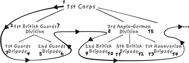
Say that we visit a node for the very first time. For instance,
in the example of Figure
7-1, after having assigned the integer 1 to the left_num value of the 1st
Corps node, we encounter (for the first time) the node
1st British Guards Division. We increase our
counter and assign 2 to left_num. Then we visit the node’s children,
encountering for the first time 1st Guards
Brigade and assigning the value of our counter, 3 at this stage, to left_num. But this node, on this example,
has no child. Because there is no child, we increment our counter and
assign its value to right_num,
which in this case takes the value 4. Then we move on to the node’s sibling,
2nd Guards Brigade. It is the same story with
this sibling. Finally, we return—our second visit—to the parent node
1st British Guards Division and can assign the
new value of our counter, which has now reached 7, to its right_num. We then proceed to the next
sibling, 3rd Anglo-German Division, and so
on.
As mentioned earlier, you can see that the [left_num, right_num] pair of any node is enclosed
within the [left_num, right_num] pair of any of its
ascendants—hence the name of nested sets. Since,
however, we have three independent trees (the Anglo-Dutch, Prussian,
and French armies), which is called in technical terms a
forest, I have had to create an artificial top
level that I have called Armies of
1815. Such an artificial top level is not required by the
other models.
Here is what we get from our example after having computed all numbers:
DESCRIPTION COMMANDER LEFT_NUM RIGHT_NUM
---------------------------- -------------------------- -------- ----------
Armies of 1815 1 1622
French Armée du Nord of 1815 Emperor Napoleon Bonaparte 870 1621
III Corps Général de Division 1237 1316
Dominique Vandamme
8th Infantry Division Général de Division Baron 1238 1253
Etienne-Nicolas Lefol
1st Brigade Général de Brigade Billard 1239 1244
(d.15th)
15th Rgmt Léger Colonel Brice 1240 1241
23rd Rgmt de Ligne Colonel Baron Vernier 1242 1243
2nd Brigade Général de Brigade Baron 1245 1248
Corsin
37th Rgmt de Ligne Colonel Cornebise 1246 1247
Division Artillery 1249 1252
7/6th Foot Artillery Captain Chauveau 1250 1251
The rows in our sample that are at the bottom level in the
hierarchy can be spotted by noticing that right_num is equal to left_num + 1.
The author of this clever method claims that it is much better
than the adjacency model because it operates on sets and that is what
SQL is all about. This is perfectly true, except that SQL is all about
unbounded sets, whereas his method relies on finite sets, in that you
must count all nodes before being able to assign the right_num value of the root. And of course,
whenever you insert a node somewhere, you must renumber both the
left_num and right_num values of all the nodes that
should be visited after the new node, as well as the right_num value of all its ascendants. The
necessity to modify many other items when you insert a new item is
exactly what happens when you store an ordered list into an array: as
soon as you insert a new value, you have to shift, on average, half
the array. The nested set model is imaginative, no doubt, but a
relational nightmare, and it is difficult to imagine worse in terms of
denormalization. In fact, the nested sets model is a pointer-based
solution, the very quagmire from which the relational approach was
designed to escape.
Walking a Tree with SQL
In order to check efficiency and performance, I have compared how each model performed with respect to the following two problems:
To find all the units under the command of the French general Dominique Vandamme (a top-down query), if possible as an indented report (which requires keeping track of the depth within the tree) or as a simple list. Note that in all cases we have an index on the commander’s name. I refer to this problem as the Vandamme query.
To find, for all regiments of Scottish Highlanders, the various units they belong to, once again with and without proper indentation (a bottom-up query). We have no index on the names of units (column
descriptionin the tables), and our only way to spot Scottish Highlanders is to look for theHighlandstring in the name of the unit, which of course means a full scan in the absence of any full-text indexing. I refer to this problem as the Highlanders query.
To ensure that the only variation from test to test was in the model used, my comparisons are all done using the same DBMS, namely Oracle.
Top-Down Walk: The Vandamme Query
In the Vandamme query, we start with the commander of the French Third Corps, General Vandamme, and want to display in an orderly fashion all units under his command. We don’t want a simple list: the structure of the army corps must be clear, as the corps is made of divisions that are themselves made of brigades that are themselves usually composed of two regiments.
Adjacency model
Writing the Vandamme query with the adjacency
model is fairly easy when using Oracle’s connect by operator. All you have to
specify is the node you wish to start from (start with) and how each two successive
rows returned relate to each other (connect
by < a column of the current
row > = prior
< a column of the previous
row >, or
connect
          by <
a
column of the previous row > = prior < a column of
the current row >, depending on whether you are walking
down or up the tree). For indentation, Oracle maintains a
pseudo-column named level that
tells you how many levels away from the starting point you are. I am
using this pseudo-column and left-padding the description with as many spaces as the
current value of level. My query
is:
    select lpad(description, length(description) + level) description,
           commander
    from adjacency_model
    connect by parent_id = prior id
    start with commander = 'Général de Division Dominique Vandamme'
And the results are:
    DESCRIPTION                     COMMANDER
    ------------------------------- -----------------------------------------------
     III Corps                      Général de Division Dominique Vandamme
      8th Infantry Division         Général de Division Baron Etienne-Nicolas Lefol
       2nd Brigade                  Général de Brigade Baron Corsin
        37th Rgmt de Ligne          Colonel Cornebise
       1st Brigade                  Général de Brigade Billard (d.15th)
        23rd Rgmt de Ligne          Colonel Baron Vernier
        15th Rgmt Léger             Colonel Brice
           ...
      10th Infantry Division        Général de Division Baron Pierre-Joseph Habert
       2nd Brigade                  Général de Brigade Baron Dupeyroux
        70th Rgmt de Ligne          Colonel Baron Maury
        22nd Rgmt de Ligne          Colonel Fantin des Odoards
        2nd (Swiss) Infantry Rgmt   Colonel Stoffel
       1st Brigade                  Général de Brigade Baron Gengoult
        88th Rgmt de Ligne          Colonel Baillon
        34th Rgmt de Ligne          Colonel Mouton
       Division Artillery
        18/2nd Foot Artillery       Captain Guérin

    40 rows selected.
Now, what about the other member in the adjacency family, the
recursive with
statement?[*] With this model, a recursive-factorized statement is
defined, which is made of the union (the union
all, to be precise) of two select statements:
The
selectthat defines our starting point, which in this particular case is:select 1 level, id, description, commander from adjacency_model where commander = 'Général de Division Dominique Vandamme'What is this solitary
1for? It represents, as the alias indicates, the depth in the tree. In contrast to the Oracleconnect byimplementation, this DB2 implementation has no system pseudo-variable to tell us where we are in the tree. We can compute our level, however, and I’ll explain more about that in just a moment.The
selectwhich defines how each child row relates to its parent row, as it is returned by this very same query that we can call, with a touch of originality,recursive_query:select parent.level + 1, child.id, child.description, child.comander from recursive_query parent, adjacency_model child where parent.id = child.parent_idNotice in this query that we add
1toparent.level. Each execution of this query represents a step down the tree. For each step down the tree, we increment our level, thus keeping track of our depth.
All that’s left is to fool around with functions to nicely indent the description, and here is our final query:
with recursive_query(level, id, description, commander)
as (select 1 level,
id,
description,
commander
from adjacency_model
where commander = 'Général de Division Dominique Vandamme'
union
          all
select parent.level + 1,
child.id,
child.description,
child.commander
from recursive_query parent,
adjacency_model child
where parent.id = child.parent_id)
select char(concat(repeat(' ', level), description), 60) description,
commander
from recursive_query
Of course, you have to be a real fan of the recursive with to be able to state without blushing
that the syntax here is natural and obvious. However, it is not too
difficult to understand once written; and it’s even rather
satisfactory, except that the query first returns General Vandamme
as expected, but then all the officers directly reporting to him,
and then all the officers reporting to the first one at the previous
level, followed by all officers reporting to the second one at the
previous level, and so on. The result is not quite the nice
top-to-bottom walk of the connect
by, showing exactly who reports to whom. I’ll hasten to
say that since ordering doesn’t belong to the relational theory,
there is nothing wrong with the ordering that you get from with, but that ordering does raise an
important question: in practice, how can we order the rows from a
hierarchical query?
Ordering the rows from a hierarchical query using recursive
with is indeed possible if, for
instance, we make the not unreasonable assumption that one parent
node never has more than 99 children and that the tree is not
monstrously deep. Given these caveats, what we can do is associate
with each node a number that indicates where it is located in the
hierarchy—say 1.030801--to mean
the first child (the two rightmost digits) of the eighth child (next
two digits, from right to left) of the third child of the root node.
This assumes, of course, that we are able to order siblings, and we
may not always be able to assign any natural ordering to them.
Sometimes it is necessary to arbitrarily assign an order to each
sibling using, possibly, an OLAP function such as row_number( ) .
We can therefore slightly modify our previous query to arbitrarily assign an order to siblings and to use the just-described technique for ordering the result rows:
with recursive_query(level, id,rank, description, commander) as (select 1, id,cast(1 as double), description, commander from adjacency_model where commander = 'Général de Division Dominique Vandamme' union all select parent.level + 1, child.id,parent.rank + ranking.sn / power(100.0, parent.level), child.description, child.commander from recursive_query parent, (select id, row_number( ) over (partition by parent_id order by description) sn from adjacency_model) ranking, adjacency_model child where parent.id =child.parent_idand child.id = ranking.id) select char(concat(repeat(' ', level), description), 60) description, commander from recursive_queryorder by rank
We might fear that the ranking query that appears as a recursive
component of the query would be executed for each node in the tree
that we visit, returning the same result set each time. This isn’t
the case. Fortunately, the optimizer is smart enough not to execute
the ranking query more than is
necessary, and we get:
DESCRIPTION COMMANDER
----------------------------- ----------------------------------------------
III Corps Général de Division Dominique Vandamme
10th Infantry Division Général de Division Baron Pierre-Joseph Habert
1st Brigade Général de Brigade Baron Gengoult
34th Rgmt de Ligne Colonel Mouton
88th Rgmt de Ligne Colonel Baillon
2nd Brigade Général de Brigade Baron Dupeyroux
22nd Rgmt de Ligne Colonel Fantin des Odoards
2nd (Swiss) Infantry Rgmt Colonel Stoffel
70th Rgmt de Ligne Colonel Baron Maury
Division Artillery
18/2nd Foot Artillery Captain Guérin
11th Infantry Division Général de Division Baron Pierre Berthézène
...
23rd Rgmt de Ligne Colonel Baron Vernier
2nd Brigade Général de Brigade Baron Corsin
37th Rgmt de Ligne Colonel Cornebise
Division Artillery
7/6th Foot Artillery Captain Chauveau
Reserve Artillery Général de Division Baron Jérôme Doguereau
1/2nd Foot Artillery Captain Vollée
2/2nd Rgmt du Génie
The result is not strictly identical to the connect by case, simply because we have
ordered siblings by alphabetical order on the description column, while we didn’t order
siblings at all with connect by
(we could have ordered them by adding a special clause). But
otherwise, the very same hierarchy is displayed.
While the result of the with query is logically equivalent to that
of the connect by query, the
with query is a splendid example
of nightmarish, obfuscated SQL, which in comparison makes the
five-line connect by query look
like a model of elegant simplicity. And even if on this particular
example performance is more than acceptable, one can but wonder with
some anguish at what it might be on very large tables. Must we
disregard the recursive with as a
poor, substandard implementation of the superior connect by? Let’s postpone conclusions
until the end of this chapter.
The ranking number we built in the recursive query is nothing more than a numerical representation of the materialized path. It is therefore time to check how we can display the troops under the command of General Vandamme using a simple materialized path implementation.
Materialized path model
Our query is hardly more difficult to write under the
materialized path model —but for the level, which is derived from the path
itself. Let’s assume just for an instant that we have at hand a
function named mp_depth( ) that
returns the number of hierarchical levels between the current node
and the top of the tree. We can write a query as:
select lpad(a.description, length(a.description)
+ mp_depth(...)) description,
a.commander
from materialized_path_model a,
materialized_path_model b
where a.materialized_path like b.materialized_path || '%'
and b.commander = 'Général de Division Dominique Vandamme')
order by a.materialized_path
Before dealing with the mp_depth(
) function, I’ll note a few traps.
In my example, I have chosen to start the materialized path with
A for the Anglo-Dutch army,
P for the Prussian one, and
F for the French one. That first letter is then
followed by dot-separated digits. Thus, the 12th Dutch line
battalion, under the command of Colonel Bagelaar, is A.1.4.2.3, while the 11th Régiment of
Cuirassiers of Colonel Courtier is F.9.1.2.2. Ordering by materialized path
can lead to the usual problems of alphabetical sorts of strings of
digits, namely that 10.2 will be
returned before 2.3; however, I
should stress that, since the separator has a lower code (in ASCII
at least) than 0, then the order
of levels will be respected. The sort may not, however respect the
order of siblings implied by the path. Does that matter? I don’t
believe that it does because sibling order is usually information
that can be derived from something other than the materialized path
itself (for instance, brothers and sisters can be ordered by their
birth dates, rather than by the path). Be careful with the approach
to sorting that I’ve used here. The character encoding used by your
database might throw off the results.
What about our mysterious mp_depth(
) function now? The hierarchical
difference between any commander under General Vandamme and General
Vandamme himself can be defined as the difference between the
absolute levels (i.e., counting down from the root of the tree) of
the unit commanded by General Vandamme and any of the underlying
units. How then can we determine the absolute level? Well, by
counting the dots.
To count the dots, the easiest thing to do is probably to
start with suppressing them, with the help of
the replace( ) function that you
find in the SQL dialect of all major products. All you have to do
next is subtract the length of the string
without the dots from the length of the string
with the dots, and you get exactly what you
want, the dot-count:
length((materialized_path) - length(replace(materialized_path, '.', ''))
If we check the result of our dot-counting algorithm for the author of the epigraph that adorns Chapter 6 (a cavalry colonel at the time), here is what we get:
SQL> select materialized_path,
2 length(materialized_path) len_w_dots,
3 length(replace(materialized_path, '.', '')) len_wo_dots,
4 length(materialized_path) -
5 length(replace(materialized_path, '.', '')) depth,
6 commander
7 from materialized_path_model
8 where commander = 'Colonel de Marbot'
9 /
MATERIALIZED_PATH LEN_W_DOTS LEN_WO_DOTS DEPTH COMMANDER
----------------- ---------- ----------- ---------- ------------------
F.1.5.1.1 9 5 4 Colonel de Marbot
Et voilà.
Nested sets model
Finding all the units under the command of General
Vandamme is very easy under the nested sets model, since the model
requires us to have numbered our nodes in such a way that the
left_num and right_num of a node bracket are the
left_num and right_num of all descendants. All we have
to write is:
select a.description,
a.commander
from nested_sets_model a,
nested_sets_model b
where a.left_num between b.left_num and b.right_num
and b.commander = 'Général de Division Dominique Vandamme'
All? Not quite. We have no indentation here. How do we get the
level? Unfortunately, the only way we have to get the depth of a
node (from which indentation is derived) is by counting how many
nodes we have between that node and the root. There is no way to
derive depth from left_num and
right_num (in contrast to the
materialized path model).
If we want to display an indented list under the nested sets
model, then we must join a third time with our nested_sets_model table, for the sole
purpose of computing the depth:
select lpad(description, length(description) + depth) description,
commander
from (select count(c.left_num) depth,
a.description,
a.commander,
a.left_num
from nested_sets_model a,
nested_sets_model b,
nested_sets_model c
where a.left_num between c.left_num and c.right_num
and c.left_num between b.left_num and b.right_num
and b.commander = 'Général de Division Dominique Vandamme'
group by a.description,
a.commander,
a.left_num)
order by left_num
The simple addition of the indentation requirement makes the
query, as with (sic) the recursive with(
), somewhat illegible.
Comparing the Vandamme query under the various models
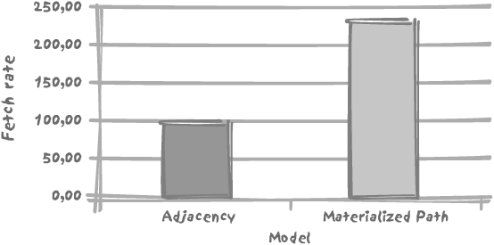
After having checked that all queries were returning the same 40 rows properly indented, I then ran each of the queries 5,000 times in a loop (thus returning a total of 200,000 rows). I have compared the number of rows returned per second, taking the adjacency model as our 100-mark reference. You see the results in Figure 7-2.
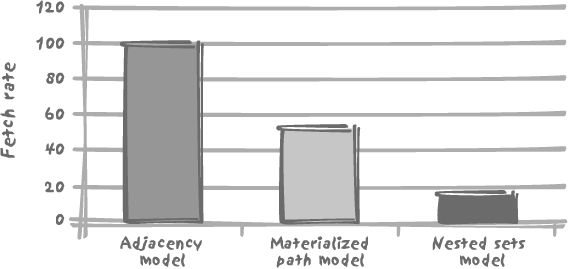
As Figure 7-2
shows, for the Vandamme query, the adjacency model, in which the
tree is walked using connect by,
outperforms the competition despite the procedural nature of
connect by. The materialized path
makes a decent show, but probably suffers from the function calls to
compute the depth and therefore the indentation. The cost of a
nicely indented output is even more apparent with the nested sets
model, where the obvious performance killer is the computation of
the depth through an additional join and a group by. One might cynically suggest
that, since this model is totally hard-wired, static, and
non-relational, we might as well go whole hog in ignoring relational
design tenets and store the depth of each node relative to the root.
Doing so would certainly improve our query’s performance, but at a
horrendous cost in terms of maintenance.
Bottom-Up Walk: The Highlanders Query
As I said earlier, looking for the Highland string within the description attributes will necessarily lead to a full scan of the table. But let’s write our query with each of the models in turn, and then we’ll consider the resulting performance implications.
Adjacency model
The Highlanders query is very straightforward to write using
connect
          by
, and once again we use
the dynamically computed level
pseudo-column to indent our result properly. Note that level was previously giving the depth, and
now it returns the height since it is always computed from our
starting point, and that we now return the parent after the
child:
    select lpad(description, length(description) + level) description,
           commander
    from adjacency_model
    connect by id = prior parent_id
    start with description like '%Highland%'
And here is the result that we get:
    DESCRIPTION                        COMMANDER
    ---------------------------------- ----------------------------------------
     2/73rd (Highland) Rgmt of Foot    Lt-Colonel William George Harris
      5th British Brigade              Major-General Sir Colin Halkett
       3rd Anglo-German Division       Lt-General Count Charles von Alten
        I Corps                        Prince William of Orange
         The Anglo-Allied Army of 1815 Field Marshal Arthur Wellesley, Duke of
                                       Wellington
     1/71st (Highland) Rgmt of Foot    Lt-Colonel Thomas Reynell
      British Light Brigade            Major-General Frederick Adam
       2nd Anglo-German Division       Lt-General Sir Henry Clinton
        II Corps                       Lieutenant-General Lord Rowland Hill
         The Anglo-Allied Army of 1815 Field Marshal Arthur Wellesley, Duke of
                                       Wellington
     1/79th (Highland) Rgmt of Foot    Lt-Colonel Neil Douglas
      8th British Brigade              Lt-General Sir James Kempt
       5th Anglo-German Division       Lt-General Sir Thomas Picton (d.18th)
        General Reserve                Duke of Wellington
         The Anglo-Allied Army of 1815 Field Marshal Arthur Wellesley, Duke of
                                       Wellington
     1/42nd (Highland) Rgmt of Foot    Colonel Sir Robert Macara (d.16th)
      9th British Brigade              Major-General Sir Denis Pack
       5th Anglo-German Division       Lt-General Sir Thomas Picton (d.18th)
        General Reserve                Duke of Wellington
         The Anglo-Allied Army of 1815 Field Marshal Arthur Wellesley, Duke of
                                       Wellington
     1/92nd (Highland) Rgmt of Foot    Lt-Colonel John Cameron
      9th British Brigade              Major-General Sir Denis Pack
       5th Anglo-German Division       Lt-General Sir Thomas Picton (d.18th)
        General Reserve                Duke of Wellington
         The Anglo-Allied Army of 1815 Field Marshal Arthur Wellesley, Duke of
                                       Wellington

    25 rows selected.
The non-relational nature of connect
by appears plainly enough: our result is not a relation,
since we have duplicates. The name of the Duke of Wellington appears
eight times, but in two different capacities, five times (as many
times as we have Highland regiments) as commander-in-chief, and
three as commander of the General Reserve. Twice—once as commander
of the General Reserve and once as commander-in-chief—would have
been amply sufficient. Can we easily remove the duplicates? No we
cannot, at least not easily. If we apply a distinct, the DBMS will sort our result to
get rid of the duplicate rows and will break the hierarchical order.
We get a result that somehow answers the question. But you can take
it or leave it according to the details of your requirements.
Materialized path model
The Highlanders query is slightly more difficult to write under the materialized path model . Identifying the proper rows and indenting them correctly is easy:
select lpad(a.description, length(a.description)
+ mp_depth(b.materialized_path)
- mp_depth(a.materialized_path)) description,
a.commander
from materialized_path_model a,
materialized_path_model b
where b.materialized_path like a.materialized_path || '%'
and b.description like '%Highland%')
However, we have two issues to solve:
We have duplicates, as with the adjacency model.
The order of rows is not the one we want.
Paradoxically, the second issue is the reason why we can solve
the first one easily; since we shall have to find a means of
correctly ordering anyway, adding a distinct will break nothing in this case.
How can we order correctly? As usual, by using the materialized path
as our sort key. By adding these two elements and pushing the query
into the from clause so as to be
able to sort by materialized_path
without displaying the column, we get:
select description, commander
from (select distinct lpad(a.description, length(a.description)
+ mp_depth(b.materialized_path)
- mp_depth(a.materialized_path)) description,
a.commander,
a.materialized_path
from materialized_path_model a,
materialized_path_model b
where b.materialized_path like a.materialized_path || '%'
and b.description like '%Highland%')
order by materialized_path desc
which displays:
DESCRIPTION COMMANDER
---------------------------------- ----------------------------------------
1/92nd (Highland) Rgmt of Foot Lt-Colonel John Cameron
1/42nd (Highland) Rgmt of Foot Colonel Sir Robert Macara (d.16th)
9th British Brigade Major-General Sir Denis Pack
1/79th (Highland) Rgmt of Foot Lt-Colonel Neil Douglas
8th British Brigade Lt-General Sir James Kempt
5th Anglo-German Division Lt-General Sir Thomas Picton (d.18th)
General Reserve Duke of Wellington
1/71st (Highland) Rgmt of Foot Lt-Colonel Thomas Reynell
British Light Brigade Major-General Frederick Adam
2nd Anglo-German Division Lt-General Sir Henry Clinton
II Corps Lieutenant-General Lord Rowland Hill
2/73rd (Highland) Rgmt of Foot Lt-Colonel William George Harris
5th British Brigade Major-General Sir Colin Halkett
3rd Anglo-German Division Lt-General Count Charles von Alten
I Corps Prince William of Orange
The Anglo-Allied Army of 1815 Field Marshal Arthur Wellesley, Duke of
Wellington
16 rows selected.
This is a much nicer and more compact result than is achieved with the adjacency model. However, I should point out that a condition such as:
where b.materialized_path like a.materialized_path || '%'
where we are looking for a row in the table aliased by
a, knowing the rows in the table
aliased by b, is something that,
generally speaking, may be slow because we can’t make efficient use
of the index on the column. What we would like to do, to make
efficient use of the index, is the opposite, looking for b.materialized_path knowing a.materialized_path. There are ways to
decompose a materialized path into the list of the materialized
paths of the ancestors of the node (see Chapter 11), but that operation is
not without cost. On our sample data, the query we have here was
giving far better results than decomposing the material path so as
to perform a more efficient join with the materialized path of each
ancestor. However, this might not be true against several million
rows.
Nested sets model
Once again, what hurts this model is that the depth must be
dynamically computed, and that computation is a rather heavy
operation. Since the Highlanders query is a bottom-up query, we must
take care not to display the artificial root node (easily identified
by left_num = 1) that we have had
to introduce. Moreover, I have had to hard-code the maximum depth
(6) to be able to indent properly. In our display, top levels are
more indented than bottom levels, which means that padding is
inversely proportional to depth. Since the depth is difficult to
get, defining the indentation as 6 -
depth was the simplest way to achieve the required
result.
As with the materialized path model, we have to reorder
anyway, so we have no scruple about applying a distinct to get rid of duplicate rows.
Here’s the query:
select lpad(description, length(description) + 6 - depth) description,
commander
from (select distinct b.description,
b.commander,
b.left_num,
(select count(c.left_num)
from nested_sets_model c
where b.left_num between c.left_num
and c.right_num) depth
from nested_sets_model a,
nested_sets_model b
where a.description like '%Highland%'
and a.left_num between b.left_num and b.right_num
and b.left_num > 1)
order by left_num desc
This query displays exactly the same result as does the materialized path query in the preceding section.
Comparing the various models for the Highlanders query
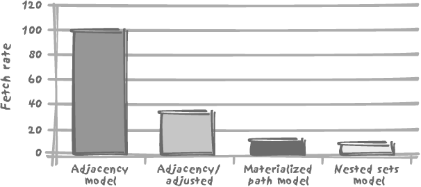
I have applied the same test to the Highlanders query as to the Vandamme query earlier, running each of the queries 5,000 times, with a minor twist: the adjacency model, as we have seen, returns duplicate rows that we cannot get rid of. My test returns 5,000 times 25 rows for the adjacency model, and 5,000 times 16 rows with the other models, because they are the only rows of interest. If we measure performance as a simple number of rows returned by unit of time, with the adjacency model we are also counting many rows that we are not interested in. I have therefore added an adjusted adjacency model, for which performance is measured as the number of rows of interest—the rows returned by the other two models—per unit of time. The result is given in Figure 7-3.
It is quite obvious from Figure 7-3 that the adjacency model outperforms the two other models by a very wide margin before adjustment, and still by a very comfortable margin after adjustment. Also notice that the materialized path model is still faster than the nested sets model, but only marginally so.
We therefore see that, in spite of its procedural nature, the
implementation of the connect by
works rather well, both for top-down and bottom-up queries, provided
of course that columns are suitably indexed. However, the return of
duplicate rows in bottom-up queries when there are several starting
points can prove to be a practical nuisance.
When connect by or a
recursive with is not available,
the materialized path model makes a good substitute. It is
interesting to see that it performs better than the totally
hard-wired nested sets model.
When designing tables to store hierarchical data, there are a number of mistakes to avoid, some of which are made in our example:
- The materialized path should in no way be the key, even if it is unique.
It is true that strong hierarchies are not usually associated with dynamic environments, but you are not defined by your place in a hierarchy.
- The materialized path should not imply any ordering of siblings.
Ordering does not belong to a relational model; it is simply concerned with the presentation of data. You must not have to change anything in other rows when you insert a new node or delete an existing one (which is probably the biggest practical reason, forgetting about all theoretical reasons, for not using the nested sets model). It is always easy to insert a node as the parents’ last child. You can order everything first by sorting on the materialized path of the parent, and then on whichever attribute looks suitable for ordering the siblings.
- The choice of the encoding is not totally neutral.
The choice is not neutral because whether you must sort by the materialized path or by the parent’s materialized path, you must use that path as a sort key. The safest approach is probably to use numbers left padded with zeroes, for instance
001.003.004.005(note that if we always use three positions for each number, the separator can go). You might be afraid of the materialized path’s length; but if we assume that each parent never has more than 100 children numbered from 0 to 99, 20 characters allow us to store a materialized path for up to 10 levels, or trees containing up to 10010 nodes—probably more than needed.
Aggregating Values from Trees
Now that you know how to deal with trees, let’s look at how you can aggregate values held in tree structures. Most cases for the aggregation of values held in hierarchical structures fall into two categories: aggregation of values stored in leaf nodes and propagation of percentages across various levels in the tree.
Aggregation of Values Stored in Leaf Nodes
In a more realistic example than the one used to illustrate the Vandamme and Highlanders queries, nodes carry information—especially the leaf nodes. For instance, regiments should hold the number of their soldiers, from which we can derive the strength of every fighting unit.
Modeling head counts
If we take the same example we used previously, restricting it to a subset of the French Third Corps of General Vandamme and only descending to the level of brigades, a reasonably correct representation (as far as we can be correct) would be the tables described in the following subsections.
UNITS. Each row in the
units table describes the various
levels of aggregation (army corps, division, brigade) as in tables
adjacency_model, materialized_path_models, or nested_sets_model, but without any
attribute to specify how each unit relates to a larger unit:
ID NAME COMMANDER
-- -------------------------- -----------------------------------------------
1 III Corps Général de Division Dominique Vandamme
2 8th Infantry Division Général de Division Baron Etienne-Nicolas Lefol
3 1st Brigade Général de Brigade Billard
4 2nd Brigade Général de Brigade Baron Corsin
5 10th Infantry Division Général de Division Baron Pierre-Joseph Habert
6 1st Brigade Général de Brigade Baron Gengoult
7 2nd Brigade Général de Brigade Baron Dupeyroux
8 11th Infantry Division Général de Division Baron Pierre Berthézène
9 1st Brigade Général de Brigade Baron Dufour
10 2nd Brigade Général de Brigade Baron Logarde
11 3rd Light Cavalry Division Général de Division Baron Jean-Simon Domont
12 1st Brigade Général de Brigade Baron Dommanget
13 2nd Brigade Général de Brigade Baron Vinot
14 Reserve Artillery Général de Division Baron Jérôme Doguereau
Since the link between units is no longer stored in this table, we need an additional table to describe how the different nodes in the hierarchy relate to each other.
UNIT_LINKS_ADJACENCY. We
may use the adjacency model once more, but this time links between
the various units are stored separately from other attributes, in an
adjacency list, in other words a list that
associates to the (technical) identifier of each row, id, the identifier of the parent row. Such
a list isolates the structural information. Our unit_links_adjacency table looks like
this:
ID PARENT_ID
---------- ----------
2 1
3 2
4 2
5 1
6 5
7 5
8 1
9 8
10 8
11 1
12 11
13 11
14 1
UNIT_LINKS_PATH. But you
have seen that an adjacency list wasn’t the only way to describe the
links between the various nodes in a tree. Alternatively, we may as
well store the materialized path, and we can put that into the
unit_links_path table:
ID PATH
---------- -----------------
1 1
2 1.1
3 1.1.1
4 1.1.2
5 1.2
6 1.2.1
7 1.2.2
8 1.3
9 1.3.1
10 1.3.2
11 1.4
12 1.4.1
13 1.4.2
14 1.5
UNIT_STRENGTH. Finally, our
historical source has provided us with the number of men in each of
the brigades—the lowest unit level in our sample. We’ll put that
information into our unit_strength table:
ID MEN
---------- ----------
3 2952
4 2107
6 2761
7 2823
9 2488
10 2050
12 699
13 318
14 152
Computing head counts at every level
With the adjacency model, it is typically quite easy to retrieve the number of men we have recorded for the third corps; all we have to write is a simple query such as:
select sum(men)
from unit_strength
where id in (select id
from unit_links_adjacency
connect by prior id = parent_id
start with parent_id = 1)
Can we, however, easily get the head count at each level, for example, for each division (the battle unit composed of two brigades) as well? Certainly, in the very same way, just by changing the starting point—using the identifier of each division each time instead of the identifier of the French Third Corps.
We are now facing a choice: either we have to code procedurally in our application, looping on all fighting units and summing up what needs to be summed up, or we have to go for the full SQL solution, calling the query that computes the head count for each and every row returned. We need to slightly modify the query so as to return the actual head count each time the value is directly known, for example, for our lowest level, the brigade. For instance:
    select u.name,
           u.commander,
           (select sum(men)
            from unit_strength
            where id in (select id
                         from unit_links_adjacency
                         connect by parent_id = prior id
                         start with parent_id = u.id)
               or id = u.id) men
    from units u
It is not very difficult to realize that we shall be hitting
again and again the very same rows, descending the very same tree
from different places. Understandably, on large volumes, this
approach will kill performance. This is where the procedural nature
of connect by, which leaves us
without a key to operate on (something I pointed out when I could
not get rid of duplicates without destroying the order I wanted),
leaves us no other choice than to adopt procedural processing when
performance becomes a critical issue; “for all they that take the
procedure shall perish with the procedure.”
We are in a slightly better position with the materialized
path here, if we are ready to allow a touch of black magic that I
shall explain in Chapter 11.
I have already referred to the explosion of
links; it is actually possible, even if it is not a pretty sight, to
write a query that explodes unit_links_path. I have called this view
exploded_links_path and here is
what it displays when it is queried:
    SQL> select * from exploded_links_path;

            ID   ANCESTOR      DEPTH
    ---------- ---------- ----------
            14          1          1
            13          1          2
            12          1          2
            11          1          1
            10          1          2
             9          1          2
             8          1          1
             7          1          2
             6          1          2
             5          1          1
             4          1          2
             3          1          2
             2          1          1
             4          2          1
             3          2          1
             7          5          1
             6          5          1
            10          8          1
             9          8          1
            13         11          1
            12         11          1
depth gives the generation
gap between id and ancestor.
When you have this view, it becomes a trivial matter to sum up over all levels (bar the bottom one in this case) in the hierarchy:
    select u.name, u.commander, sum(s.men) men
    from units u,
         exploded_links_path el,
         unit_strength s
    where u.id = el.ancestor
      and el.id = s.id
    group by u.name, u.commander
which returns:
    NAME                       COMMANDER                              MEN
    -------------------------- -------------------------------------- -----
    III Corps                  Général de Division Dominique Vandamme 16350
    8th Infantry Division      Général de Division Baron Etienne-      5059
                               Nicolas Lefol
    10th Infantry Division     Général de Division Baron Pierre        5584
                               Joseph Habert
    11th Infantry Division     Général de Division Baron Pierre        4538
                               Berthézène
    3rd Light Cavalry Division Général de Division Baron Jean-Simon    1017
                               Domont
(We can add, through a union, a join between units and unit_strength to see units displayed for
which nothing needs to be computed.)
I ran the query 5,000 times to determine the numerical strength for all units, and then I compared the number of rows returned per unit time. As might be expected, the result shows that the adjacency model, which had so far performed rather well, bites the dust, as is illustrated in Figure 7-4.
Propagation of Percentages Across Different Levels
Must we conclude that with a materialized path and a pinch of adjacency where available we can solve anything more or less elegantly and efficiently? Unfortunately not, and our last example will really demonstrate the limits of some SQL implementations when it comes to handling trees.
For this case, let’s take a totally different example, and we will assume that we are in the business of potions, philters, and charms. Each of them is composed of a number of ingredients—and our recipes just list the ingredients and their percentage composition. Where is the hierarchy? Some of our recipes share a kind of “base philter” that appears as a kind of compound ingredient, as in Figure 7-5.
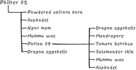
Our aim is, in order to satisfy current regulations, to display on the package of Philter #5 the names and proportions of all the basic ingredients. First, let’s consider how we can model such a hierarchy. In such a case, a materialized path would be rather inappropriate. Contrarily to fighting units that have a single, well-defined place in the army hierarchy, any ingredient, including compound ones such as Potion #9, can contribute to many preparations. A path cannot be an attribute of an ingredient. If we decide to “flatten” compositions and create a new table to associate a materialized path to each basic ingredient in a composition, any change brought to Potion #9 would have to ripple through potentially hundreds of formulae, with the unacceptable risk in this line of business of one change going wrong.
The most natural way to represent such a structure is therefore to say that our philter contains so much of powdered unicorn horn, so much of asphodel, and so much of Potion #9 and so forth, and to include the composition of Potion #9.
Figure 7-6
illustrates one way we can model our database. We have a generic
components table with two subtypes,
recipes and basic_ingredients, and a composition table storing the quantity of a
component (a recipe or a basic ingredient) that appears in each
recipe.
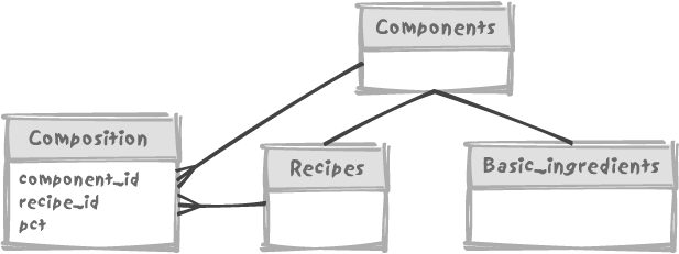
However, Figure
7-6’s design is precisely where an approach such as connect by becomes especially clunky.
Because of the procedural nature of the connect by operator, we can include only two
levels, which could be enough for the case of Figure 7-5, but not in a general
case. What do I mean by including two levels? With connect by we have the visibility of two
levels at once, the current level and the parent level, with the
possible exception of the root level. For instance:
    SQL> select connect_by_root recipe_id root_recipe,
      2         recipe_id,
      3         prior pct,
      4         pct
      5         component_id
      6  from composition
      7  connect by recipe_id = prior component_id
      8  /

    ROOT_RECIPE  RECIPE_ID   PRIORPCT          PCT COMPONENT_ID
    ----------- ---------- ---------- ------------ ------------
             14         14                       5            3
             14         14                      20            7
             14         14                      15            8
             14         14                      30            9
             14         14                      20           10
             14         14                      10            2
             15         15                      30           14
             15         14         30            5            3
             15         14         30           20            7
             15         14         30           15            8
             15         14         30           30            9
     ...
In this example, root_recipe
refers to the root of the tree. We can handle simultaneously the
percentage of the current row and the percentage of the prior row, in
tree-walking order, but we have no easy way to sum up, or in this
precise case, to multiply values across a hierarchy, from top to
bottom.
The requirement for propagating percentages across levels is,
however, a case where a recursive with statement is particularly useful. Why?
Remember that when we tried to display the underlings of General
Vandamme we had to compute the level to know how deep we were in the
tree, carrying the result from level to level across our walk. That
approach might have seemed cumbersome then. But that same approach is
what will now allow us to pull off an important trick. The great
weakness of connect by is that at
one given point in time you can only know two generations: the current
row (the child) and its parent. If we have only two levels, if Potion
#9 contains 15% of Mandragore and Philter #5 contains 30% of Potion
#9, by accessing simultaneously the child (Potion #9) and the parent
(Philter #5) we can easily say that we actually have 15% of 30%—in
other words, 4.5% of Mandragore in Philter #5. But what if we have
more than two levels? We may find a way to compute how much of each
individual ingredient is contained in the final products with
procedures, either in the program that accesses the database, or by
invoking user-defined functions to store temporary results. But we
have no way to make such a computation through plain SQL.
“What percentage of each ingredient does a formula contain?” is
a complicated question. The recursive with makes answering it a breeze. Instead of
computing the current level as being the parent level plus 1, all we
have to do is compute the actual percentage as being the current
percentage (how much Mandragore we have in Potion #9) multiplied by
the parent percentage (how much Potion #9 we have in Philter #5). If
we assume that the names of the components are held in the components table, we can write our recursive
query as follows:
    with recursive_composition(actual_pct, component_id)
    as (select a.pct,
               a.component_id
        from composition a,
             components b
        where b.component_id = a.recipe_id
          and b.component_name = 'Philter #5'
        union all
        select parent.pct * child.pct,
               child.component_id
        from recursive_composition parent,
             composition child
        where child.recipe_id = parent.component_id)
Let’s say that the components
table has a component_type column
that contains I for a basic
ingredient and R for a recipe. All
we have to do in our final query is filter (with an
f ) recipes out, and, since the same basic
ingredient can appear at various different levels in the hierarchy,
aggregate per ingredient:
    select x.component_name, sum(y.actual_pct)
    from recursive_composition y,
           components x
    where x.component_id = y.component_id
        and x.component_type = 'I'
    group by x.component_name
As it happens, even if the adjacency model looks like a fairly
natural way to represent hierarchies, its two implementations are in
no way equivalent, but rather complementary. While connect by may superficially look easier
(once you have understood where prior goes) and is convenient for displaying
nicely indented hierarchies, the somewhat tougher recursive with allows you to process much more complex
questions relatively easily—and those complex questions are the type
more likely to be encountered in real life. You only have to check the
small print on a cereal box or a toothpaste tube to notice some
similarities with the previous example of composition analysis.
In all other cases, including that of a DBMS that implements a
connect by, our only hope of
generating the result from a “single SQL statement” is by writing a
user-defined function, which has to be recursive if the DBMS cannot
walk the tree.
Important
A more complex tree walking syntax may make a more complex question easier to answer in pure SQL.
While the methods described in this chapter can give reasonably satisfactory results against very small amounts of data, queries using the same techniques against very large volumes of data may execute “as slow as molasses.” In such a case, you might consider a denormalization of the model and a trigger-based “flattening” of the data. Many, including myself, frown upon denormalization. However, I am not recommending that you consider denormalizing for the oft-cited inherent slowness of the relational model, so convenient for covering up incompetent programming, but because SQL still lacks a truly adequate, scaleable processing of tree structures.
[*] First introduced in articles in DBMS Magazine (circa 1996), and much later developed in Trees and Hierarchies in SQL for Smarties (Morgan-Kauffman).
[*] Initially published on http://www.dbazine.com.
[†] Using, with his permission, the data compiled by Peter Kessler, at http://www.kessler-web.co.uk.
[*] Using this time the first product that implemented it, namely DB2.