
Chapter 12. Employment of Spies
Monitoring Performance
And he that walketh in darkness knoweth not whither he goeth..
Gospel according to St. John, 12:35
Intelligence gathering has always been an essential part of war. All database systems include monitoring facilities, each with varying degrees of sophistication. Third-party offerings are also available in some cases. All these monitoring facilities are primarily aimed at database administrators. However, when they allow you to really see what is going on inside the SQL engine, they can become formidable spies in the service of the performance-conscious developer. I should note that when monitoring facilities lack the level of detail we require, it is usually possible to obtain additional information by turning on logging or tracing. Logging or tracing necessarily entails a significant overhead, which may not be a very desirable extra load on a busy production server that is already painfully clunking along. But during performance testing, logging can provide us with a wealth of information on what to expect in production.
Detailing all or even some of the various monitoring facilities available would be both tedious and product-specific. Furthermore, such an inventory would be rapidly outdated. I shall concentrate instead on what we should monitor and why. This will provide you with an excellent opportunity for a final review of some of the key concepts introduced in previous chapters.
The Database Is Slow
Let’s first try to define the major categories of performance issues that we are likely to encounter in production—since our goal, as developers, is to anticipate and, if possible, avoid these situations. The very first manifestation of a performance issue on a production database is often a call to the database administrators’ desk to say that “the database is slow” (a useful piece of information for database administrators who may have hundreds of database servers in their care...). In a well-organized shop, the DBA will be able to check whether a monitoring tool does indeed report something unusual, and if that is the case, will be able to answer confidently “I know. We are working on the case.” In a poorly organized shop, the DBA may well give the same answer, lying diplomatically.
In all cases, the end of the call will mean the beginning of a frantic scramble for clues.
Such communications stating that “the database is slow” will usually have been motivated by one of the five following reasons:
- It’s not the database
The network is stuttering or the host is totally overloaded by something else.
Thanks for calling.
- Sudden global sluggishness
All tasks slow down, suddenly, for all users. There are two cases to consider here:
Either the performance degradation is really sudden, in which case it can often be traced to some system or DBMS change (software upgrade, parameter adjustment, or hardware configuration modification).
Or it results from a sudden inflow of queries.
The first case is not a development issue, just one of those hazards that make the life of a systems engineer or DBA so exciting. The second case is a development or specifications issue. Remember the post office of Chapter 9: when customers arrive faster than they can be serviced, queues lengthen and performance tumbles down all of a sudden. Either the original specifications were tailored too tightly and the system is facing a load it wasn’t designed for, or the application has been insufficiently stress-tested. In many cases, improving some key queries will massively decrease the average service time and may improve the situation for a negligible fraction of the cost of a hardware upgrade. Sudden global sluggishness is usually characterized by the first phone call being followed by many others.
- Sudden localized slowness
If one particular task slows down all of a sudden, locking issues should be considered. Database administrators can monitor locks and confirm that several tasks are competing for the same resources. This situation is a development and task-scheduling issue that can be improved by trying to release locks faster.
- A slow degradation of performance reaching a threshold
The threshold may first be felt by one hypersensitive user. If the load has been steadily increasing over time, the crossing of the threshold may be a warning sign of an impending catastrophe and may relate to the lengthening service queues of a sudden global sluggishness. The crossing of a threshold may also be linked to the size increase of badly indexed tables or to a degradation of physical storage after heavy delete/update operations (hanging high-water mark of a table that has inflated then deflated, a Swiss cheese-like effect resulting in much too many pages or blocks to store the data, or chaining to overflow areas). If the problem is with indexes or physical storage (or outdated statistics taking the optimizer down a wrong path), a DBA may be able to help, but the necessity for a rescue operation on a regular basis is usually the sign of poorly designed processes.
- One particularly slow query
If the application was properly tested, then the case to watch for is a dynamically built query provided with a highly unusual set of criteria. This is most likely to be a pure development issue.
Many of these events can be foreseen and prevented. If you are able to identify what loads your server, and if you are able to relate database activity to business activity, you have all the required elements to identify the weakest spots in an application. You can then focus on those weak spots during performance testing and improve them.
The Components of Server Load
Load, in information technology, ultimately boils down to a combination of excessive CPU consumption, too many input/output operations and insufficient network speed or bandwidth. It’s quite similar to the “critical tasks” of project management, where one bottleneck can result in the whole system grinding not to a halt, but to an unnaceptable level of slowness. If processes that are ready to run must wait for some other processes to release the CPU, the system is overloaded. If the CPU is idle, waiting for data to be sent across the network or to be fetched from persistent storage, the system is overloaded too.
“Overloaded,” though, mustn’t be understood as an absolute notion. Systems may be compared to human beings in respect of the fact that load is not always directly proportional to the work accomplished. As C. Northcote Parkinson remarked in Parkinson’s Law , his famous satire of bureaucratic institutions:
Thus, an elderly lady of leisure can spend the entire day in writing and dispatching a postcard [...]. The total effort that would occupy a busy man for three minutes all told may in this fashion leave another person prostrate after a day of doubt, anxiety, and toil.
Poorly developed SQL applications can very easily bring a server to its knees and yet not achieve very much. Here are a few examples (there are many others) illustrating different ways to increase the load without providing any useful work:
- Hardcoding all queries
This will force the DBMS to run parser and optimizer code for every execution, before actually performing any data access. This technique is remarkably efficient for swamping the CPU.
- Running useless queries
This is a situation more common than one would believe. It includes queries that are absolutely useless, such as a dummy query to check that the DBMS is up and running before every statement (true story), or issuing a
count(*)to check whether a row should be updated or inserted. Other useless queries also include repeatedly fetching information that is stable for the entire duration of a session, or issuing 400,000 times a day a query to fetch a currency exchange rate that is updated once every night.- Multiplying round-trips
Operating row-by-row, extensively using cursor loops , and banishing stored procedures are all excellent ways to increase the level of “chatting” between the application side and the SQL engine, wasting time on protocol issues, multiplying packets on the network and of course, as a side benefit, preventing the database optimizer from doing its work efficiently by keeping most of the mysteries of data navigation firmly hidden in the application.
Let me underline that these examples of bad use of the DBMS don’t specifically include the “bad SQL query” that represents the typical SQL performance issue for many people. The queries described in the preceding list often run fast. But even when they run at lightning speed, useless queries are always too slow: they waste resources that may be in short supply during peak activity.
There are two components that affect the load on a database server. The visible component is made up of the slow “bad SQL queries " that people are desperate to have tuned. The invisible component is the background noise of a number of queries each of acceptable speed, perhaps even including some very fast ones, that are executed over and over again. The cumulative cost of the load generated by all this background noise routinely dwarfs the individual load of most of the big bad queries. As Sir Arthur Conan Doyle put in the mouth of Sherlock Holmes:
It has long been an axiom of mine that the little things are infinitely the most important.
As the background noise is spread over time, instead of happening all of a sudden, it passes unnoticed. It may nevertheless contribute significantly to reducing the “power reserve” that may be needed during occasional bursts of activity.
Defining Good Performance
Load is one thing, performance another. Good performance proves an elusive notion to define. Using CPU or performing a large number of I/O operations is not wrong in itself; your company, presumably, didn’t buy powerful hardware with the idea of keeping it idle.
When the time comes to assess performance, there is a striking similarity between the world of databases and the world of corporate finance. You find in both worlds some longing for “key performance indicators” and magical ratio—and in both worlds, global indicators and ratios can be extremely misleading. A good average can hide distressing results during the peaks, and a significant part of the load may perhaps be traced back to a batch program that is far from optimal but that runs at a time of night when no one cares what the load is. To get a true appreciation of the real state of affairs, you must drill down to a lower level of detail.
To a large extent, getting down to the details is an exercise similar to that which is known in managerial circles as “activity-based costing.” In a company, knowing in some detail how much you spend is relatively easy. However, relating costs to benefits is an exercise fraught with difficulties, notoriously for transverse operations such as information technology. Determining if you spend the right amount on hardware, software, and staff, as well as the rubber bands and duct tape required to hold everything together is extremely difficult, particularly when the people who actually earn money are “customers” of the IT department.
Assessing whether you do indeed spend what you should has three prerequisites:
Knowing what you spend
Knowing what you get for the money
Knowing how your return on investment compares with acknowledged standards
In the following subsections, I shall consider each of these points in turn in the context of database systems.
Knowing What You Spend
In the case of database performance, what we spend means, first and foremost, how many data pages we are hitting. The physical I/Os that some people tend to focus on are an ancillary matter. If you hit a very large number of different data pages, this will necessarily entail sustained I/O activity unless your database entirely fits in memory. But CPU load is also often a direct consequence of hitting the same data pages in memory again and again. Reducing the number of data pages accessed is not a panacea, as there are cases when the global throughput is higher when some queries hit a few more pages than is strictly necessary. But as far as single indicators go, the number of data pages hit is probably the most significant one. The other cost to watch is excessive SQL statement parsing, an activity that can consume an inordinate amount of CPU (massive hardcoded insertions can easily take 75% of the CPU available for parsing alone).
Knowing What You Get
There is a quote that is famous among advertisers, a quip attributed to John Wanamaker, a 19th-century American retailer:
Half the money I spend on advertising is wasted; the trouble is I don’t know which half.
The situation is slightly better with database applications, but only superficially. You define what you get in terms of the number of rows (or bytes) returned by select statements; and similarly the number of rows affected by change operations. But such an apparently factual assessment is far from providing a true measure of the work performed on your behalf by the SQL engine, for a number of reasons:
First, from a practical point of view, all products don’t provide you with such statistics.
Second, the effort required to obtain a result set may not be in proportion to the size of the result set. As a general rule you can be suspicious of a very large number of data page hits when only a few rows are returned. However such a proportion may be perfectly legitimate when data is aggregated. It is impossible to give a hard-and-fast rule in this area.
Third, should data returned from the database for the sole purpose of using it as input to other queries be counted as useful work? What about systematically updating to
Na column in a table without using awhereclause whenNalready happens to be the value stored in most rows? In both cases, the DBMS engine performs work that can be measured in terms of bytes returned or changed. Unfortunately, most of the work performed can be avoided.
There are times when scanning large tables or executing a long-running query may be perfectly justified (or indeed inescapable). For instance, when you run summary reports on very large volumes of data, you cannot expect an immediate answer. If an immediate answer is required, then it is likely that the data model (the database representation of reality) is inappropriate to the questions you want to see answered. This is a typical case when a decision support database that doesn’t necessarily require the level of detail of the main operational database may be suitable. Remember what you saw in Chapter 1: correct modeling depends both on the data and what you want to do with the data. You may share data with your suppliers or customers and yet have a totally different database model than they do. Naturally, feeding a decision support system will require long and costly operations both on the source operational database and the target decision support database.
Because what you do with the data matters so much, you cannot judge performance if you don’t relate the load to the execution of particular SQL statements. The global picture that may be available through monitoring utilities (that most often provide cumulative counters) is not of much interest if you cannot assign to each statement its fair share of the load.
As a first stage in the process of load analysis, you must
therefore capture and collect SQL statements, and try to determine how
much each one contributes to the overall cost. It may not be important
to capture absolutely every statement. Database activity is one of
those areas where the 80/20 rule, the empirical assessment that 80% of
the consequences result from 20% of the causes, often describes the
situation rather well. Usually, much of the load comes from a small
number of SQL statements. We must be careful not to overlook the fact
that hardcoded SQL statements may distort the picture. With hardcoded
statements, the DBMS may record thousands of distinct statements where
a properly coded query would be referenced only once, even though it
might be called thousands of times, each time with differing
parameters. Such a situation can usually be spotted quite easily by
the great number of SQL statements, and sometimes by global
statistics. For instance, a procedure such as sp_trace_setevent in Transact-SQL lets you
obtain a precise count of executed cursors, reexecutions of prepared
cursors, and so on.
If nothing else is available and if you can access the SQL engine cache , a snapshot taken at a relatively low frequency of once every few minutes may in many cases prove quite useful. Big bad queries are usually hard to miss, as also are queries that are being executed dozens of times a minute. Global costs should in any case be checked in order to validate the hypothesis that what has been missed contributes only marginally to the global load. It’s when SQL statements are hardcoded that taking snapshots will probably give less satisfactory results; you should then try to get a more complete picture, either through logging (as already mentioned a high-overhead solution), or by use of less intrusive “sniffer” utilities. I should note that even if you catch all hardcoded statements, then they have to be “reverse soft-coded” by taking constant values out of the SQL text before being able to estimate the relative load, not of a single SQL statement, but of one particular SQL statement pattern.
Identifying the statements that keep the DBMS busy, though, is
only part of the story. You will miss much if you don’t then relate
SQL activity to the essential business activity of the organization
that is supported by the database. Having an idea of how many SQL
statements are issued on average each time you are processing a
customer order is more important to SQL performance than knowing the
disk transfer rate or the CPU speed under standard conditions of
temperature and pressure. For one thing, it helps you anticipate the
effect of the next advertising campaign; and if the said number of SQL
statements is in the hundreds, you can raise interesting questions
about the program (could there be, by chance, SQL statements executed
inside loops that fetch the results of other statements? Could there
be a statement that is repeatedly executed when it needs to be
executed only once?). Similarly, costly massive updates of one column in a table accompanied by near identical
numbers of equally massive updates of other columns from the same
table with similar where clauses
immediately raises the question of whether a single pass over the
table wouldn’t have been enough.
Checking Against Acknowledged Standards
Collecting SQL statements, evaluating their cost and roughly relating them to what makes a company or agency tick is an exercise that usually points you directly to the parts of the code that require in-depth review. The questionable code may be SQL statements, algorithms, or both. But knowing what you can expect in terms of improvement or how far you could or should go is a very difficult part of the SQL expert’s craft; experience helps, but even the seasoned practitioner can be left with a degree of uncertainty.
It can be useful to establish a baseline, for instance by carrying out simple insertion tests and having an idea about the rate of insertion that is sustainable on your hardware. Similarly, you should check the fetch rate that can be obtained when performing those dreaded full scans on some of the biggest tables. Comparing bare-bones rates to what some applications manage to accomplish is often illuminating: there may be an order of magnitude or more between the fetch or insert speed that the SQL engine can attain and what is achieved by application programs.
Important
Know the limits of your environment. Measure how many rows you can insert, fetch, update, or delete per unit of time on your machines.
Once you have defined a few landmarks, you can identify where you will obtain the best “return on improvement,” in terms of both relevance to business activities and technical feasibility. You can then focus on those parts of your programs and get results where it matters.
Some practitioners tend to think that as long as end users don’t complain about performance, there is no issue and therefore no time to waste on trying to make operations go faster. There is some wisdom in this attitude; but there is also some short-sightedness as well, for two reasons:
First, end users often have a surprisingly high level of tolerance for poor performance; or perhaps it would be more appropriate to say that their perception of slowness differs widely from that of someone who has a better understanding of what happens behind the scenes. End users may complain loudly about the performance of those processes of death that cannot possibly do better, and express a mild dissatisfaction about other processes when I would have long gone ballistic. A low level of complaint doesn’t necessarily mean that everything is fine, nor does vocal dissatisfaction necessarily mean that there is anything wrong with an application except perhaps trying to do too much.
Second, a slight increase in the load on a server may mean that performance will deteriorate from acceptable to unacceptable very quickly. If the environment is perfectly stable, there is indeed nothing to fear from a slight increase in load. But if your activity records a very high peak during one particular month of the year, the same program that looks satisfactory for 11 months can suddenly be the reason for riots. Here the background noise matters a lot. An already overloaded machine cannot keep on providing the same level of service when activity increases. There is always a threshold that sees mediocre performance tumbling down all of a sudden. It is therefore important to study an entire system before a burst of activity is encountered to see whether the load can be reduced by improving the code. If improving the code isn’t enough to warrant acceptable performance, it may be time to switch to bigger iron and upgrade the hardware.
Do not forget that “return on improvement” is not simply a technical matter. The perception of end users should be given the highest priority, even if it is biased and sometimes disconnected from the most severe technical issues. They have to work with the program, and ergonomics have to be taken into account. It is not unusual to meet well-meaning individuals concentrating on improving statistics rather than program throughput, let alone end-user satisfaction. These well-intentioned engineers can feel somewhat frustrated and misunderstood when end users, who only see a very local improvement, welcome the result of mighty technical efforts with lukewarm enthusiasm. An eighteenth-century author reports that somebody once said to a physician, “Well, Mr. X has died, in spite of the promise you had made to cure him.” The splendid answer from the physician was, “You were away, and didn’t check the progress of the treatment: he died cured.”
A database with excellent statistics and yet unsatisfactory performance from an end-user point of view is like a patient cured of one ailment, but who died of another. Improving performance usually means both delivering a highly visible improvement to end users, even if it affects a query that is run only once a month but that is business-critical, and the more humble, longer-term work of streamlining programs, lowering the background noise, and ensuring that the server will be able to deliver that power boost when it is needed.
Defining Performance Goals
Performance goals are often defined in terms of elapsed time, for example, “this program must run in under 2 hours.” It is better though to define them primarily in terms of business items processed by unit of time, such as “50,000 invoices per hour” or “100 loans per minute,” for several reasons:
It gives a better idea of the service actually provided by a given program.
It makes a decrease in performance more understandable to end users when it can be linked to an increase in activity. This makes meetings less stormy.
Psychologically speaking, it is slightly more exciting when trying to improve a process to boost throughput rather than diminish the elapsed time. An upward curve makes a better chart in management presentations than a downward one.
Thinking in Business Tasks
Before focusing on one particular query, don’t forget its context. Queries executed in loops are a very bad indicator of the quality of code, as are program variables with no other purpose than storing information returned from the database before passing it to another query. Database accesses are costly, and should be kept to a minimum. When you consider the way some programs are written, you are left with the impression that when their authors go shopping, they jump into their car, drive to a supermarket, park their car, walk up and down the aisles, pick a few bottles of milk, head for the checkout, get in line, pay, put the milk in the car, drive home, store the milk into the fridge, then check the next item on the shopping list before returning to the supermarket. And when a spouse complains about the time spent on shopping, the excuses given are usually the dense traffic on the road, the poor signposting of the food department, and the insufficient number of cashiers. All are valid reasons in their own right that may indeed contribute to some extent to shopping time, but possibly they are not the first issues to fix.
I have met developers who were genuinely persuaded that from a performance standpoint, multiplying simple queries was the proper thing to do; showing them that the opposite is true was extremely easy. I have also heard that very simple SQL statements that avoid joins make maintenance easier. The truth is that simplistic SQL makes it easier to use totally inexperienced (read cheaper) developers for maintenance, but that’s the only thing that can be said in defense of very elementary SQL statements. By making the most basic usage of SQL, you end up with programs full of statements that, taken one by one, look efficient, except perhaps for a handful of particularly poor performers, hastily pointed to as “the SQL statements that require tuning.” Very often, some of the statements identified as “slow” (and which may indeed be slow) are responsible for only a fraction of performance issues.
Important
Brilliantly tuned statements in a bad program operating against a badly designed database are no more effective than brilliant tactics at the service of a feeble strategy; all they can do is postpone the day of reckoning.
You cannot design efficient programs if you don’t understand that the SQL language applies to a whole subsystem of data management, and isn’t simply a set of primitives to move data between long-term and short-term memory. Database accesses are often the most performance-critical components of a program, and must be incorporated to the overall design.
In trying to make programs simpler by multiplying SQL statements, you succumb to a dangerous illusion. Complexity doesn’t originate in languages, but in business requirements. With the exclusive use of simple SQL statements, complexity doesn’t vanish, it just migrates from the SQL side to the application side, with a much increased risk of data inconsistency when the logic that should belong to the DBMS side is imbedded into the application. Moreover, it puts a significant part of processing out of reach of the DBMS optimizer.
I am not advocating the indiscriminate use of long, complex SQL statements, or a “single statement” policy. For example, the following is a case where there should have been several distinct statements, and not a single one:
insert into custdet (custcode, custcodedet, usr, seq, inddet)
select case ?
         when 'GRP' then b.codgrp
         when 'GSR' then b.codgsr
         when 'NIT' then b.codnit
         when 'GLB' then 'GLOBAL'
         else b.codetb
       end,
       b.custcode,
       ?,
       ?,
       'O'
from edic00 a,
     clidet bT
where ((b.codgrp = a.custcode
        and ? = 'GRP')
       or (b.codgsr = a.custcode
           and ? = 'GSR')
       or (b.codnit = a.custcode
           and ? = 'NIT')
       or (a.custcode = 'GLOBAL'
           and ? = 'GLB'))
   and a.seq = ?
   and b.custlvl = ?
   and b.histdat = ?
A statement where a run-time parameter is compared to a constant
is usually a statement that should have been split into several simpler
statements. In the preceding example, the value that intervenes in the
case construct is the same one that
is successively compared to GRP,
GSR, NIT, and GLB in the where clause. It makes no sense to force the
SQL engine into making numerous mutually exclusive tests and sort out a
situation that could have been cleared on the application side. In such
a case, an if ... elsif ... elsif
structure (preferably in order of decreasing probability of occurrence)
and four distinct insert ... select
statements would have been much better.
When a complex SQL statement allows you to obtain more quickly the data you ultimately need, with a small number of accesses, the situation is completely different from the preceding case. Long, complex queries are not necessarily slow; it all depends on how they are written. A developer should obviously not exceed their personal SQL skill level, and not necessarily write 300-line statements head on; but packing as much action as possible into each SQL statement should be a prerequisite to improving individual statements.
Execution Plans
When our spies (whether they are users or monitoring facilities) have directed our attention to a number of SQL statements, we need to inspect these statements more closely. Scrutinizing execution plans is one of the favorite activities of many SQL tuners, if we are to believe the high number of posts in forums or mailing lists in the form of “I have a SQL query that is particularly slow; here is the execution plan....”
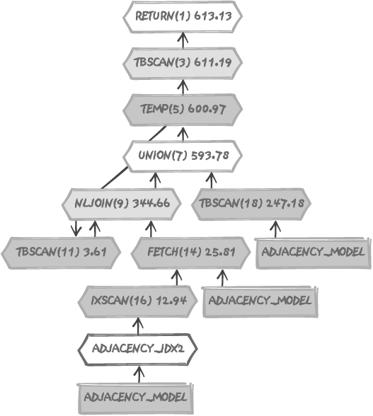
Execution plans are usually displayed either as an indented list of the various steps involved in the processing of a (usually complex) SQL statements, or under a graphical form, as in Figure 12-1. This figure displays the execution plan for one of the queries from Chapter 7. Text execution plans are far less sexy but are easier to post on forums, which must account for the enduring popularity of such plans. Knowing how to correctly read and interpret an execution plan, whether it is represented graphically or as text, is in itself a valued skill.
So far in this book, I have had very little to say on the topic of execution plans, except for a couple of examples presented here and there without any particular comment. Execution plans are tools, and different individuals have different preferences for various tools; you are perfectly allowed to have a different opinion, but I usually attach a secondary importance to execution plans. Some developers consider execution plans as the ultimate key to the understanding of performance issues. Two real-life examples will show that one may have some reasons to be less than sanguine about using execution plans as the tool of choice for improving a query.
Identifying the Fastest Execution Plan
In this section, I am going to test your skills as an interpreter of execution plans. I’m going to show three execution plans and ask you to choose which is the fastest. Ready? Go, and good luck!
Our contestants
The following execution plans show how three variants of the same query are executed:
- Plan 1
Execution Plan
----------------------------------------------------------
   0      SELECT STATEMENT
   1    0   SORT (ORDER BY)
   2    1     CONCATENATION
   3    2       NESTED LOOPS
   4    3         HASH JOIN
   5    4           HASH JOIN
   6    5             TABLE ACCESS (FULL) OF 'TCTRP'
   7    5             TABLE ACCESS (BY INDEX ROWID) OF 'TTRAN'
   8    7               INDEX (RANGE SCAN) OF 'TTRANTRADE_DATE' (NON-UNIQUE)
   9    4           TABLE ACCESS (BY INDEX ROWID) OF 'TMMKT'
  10    9             INDEX (RANGE SCAN) OF 'TMMKTCCY_NAME' (NON-UNIQUE) ...
  11    3         TABLE ACCESS (BY INDEX ROWID) OF 'TFLOW'
  12   11           INDEX (RANGE SCAN) OF 'TFLOWMAIN' (UNIQUE)
  13    2       NESTED LOOPS
  14   13         HASH JOIN
  15   14           HASH JOIN
  16   15             TABLE ACCESS (FULL) OF 'TCTRP'
  17   15             TABLE ACCESS (BY INDEX ROWID) OF 'TTRAN'
  18   17               INDEX (RANGE SCAN) OF 'TTRANLAST_UPDATED' (NON-UNIQUE)
  19   14           TABLE ACCESS (BY INDEX ROWID) OF 'TMMKT'
  20   19             INDEX (RANGE SCAN) OF 'TMMKTCCY_NAME' (NON-UNIQUE)
  21   13         TABLE ACCESS (BY INDEX ROWID) OF 'TFLOW'
  22   21           INDEX (RANGE SCAN) OF 'TFLOWMAIN' (UNIQUE)
- Plan 2
Execution Plan
----------------------------------------------------------
   0      SELECT STATEMENT
   1    0   SORT (ORDER BY)
   2    1     CONCATENATION
   3    2       NESTED LOOPS
   4    3         NESTED LOOPS
   5    4           NESTED LOOPS
   6    5             TABLE ACCESS (BY INDEX ROWID) OF 'TTRAN'
   7    6               INDEX (RANGE SCAN) OF 'TTRANTRADE_DATE' (NON-UNIQUE)
   8    5             TABLE ACCESS (BY INDEX ROWID) OF 'TMMKT'
   9    8               INDEX (UNIQUE SCAN) OF 'TMMKTMAIN' (UNIQUE)
  10    4           TABLE ACCESS (BY INDEX ROWID) OF 'TFLOW'
  11   10             INDEX (RANGE SCAN) OF 'TFLOWMAIN' (UNIQUE)
  12    3         TABLE ACCESS (BY INDEX ROWID) OF 'TCTRP'
  13   12           INDEX (UNIQUE SCAN) OF 'TCTRPMAIN' (UNIQUE)
  14    2       NESTED LOOPS
  15   14         NESTED LOOPS
  16   15           NESTED LOOPS
  17   16             TABLE ACCESS (BY INDEX ROWID) OF 'TTRAN'
  18   17               INDEX (RANGE SCAN) OF 'TTRANLAST_UPDATED' (NON-UNIQUE)
  19   16             TABLE ACCESS (BY INDEX ROWID) OF 'TMMKT'
  20   19               INDEX (UNIQUE SCAN) OF 'TMMKTMAIN' (UNIQUE)
  21   15           TABLE ACCESS (BY INDEX ROWID) OF 'TFLOW'
  22   21             INDEX (RANGE SCAN) OF 'TFLOWMAIN' (UNIQUE)
  23   14         TABLE ACCESS (BY INDEX ROWID) OF 'TCTRP'
  24   23           INDEX (UNIQUE SCAN) OF 'TCTRPMAIN' (UNIQUE)
- Plan 3
Execution Plan
----------------------------------------------------------
   0      SELECT STATEMENT
   1    0   SORT (ORDER BY)
   2    1     NESTED LOOPS
   3    2       NESTED LOOPS
   4    3         NESTED LOOPS
   5    4           TABLE ACCESS (BY INDEX ROWID) OF 'TMMKT'
   6    5             INDEX (RANGE SCAN) OF 'TMMKTCCY_NAME' (NON-UNIQUE)
   7    4           TABLE ACCESS (BY INDEX ROWID) OF 'TTRAN'
   8    7             INDEX (UNIQUE SCAN) OF 'TTRANMAIN' (UNIQUE)
   9    3         TABLE ACCESS (BY INDEX ROWID) OF 'TCTRP'
  10    9           INDEX (UNIQUE SCAN) OF 'TCTRPMAIN' (UNIQUE)
  11    2       TABLE ACCESS (BY INDEX ROWID) OF 'TFLOW'
  12   11         INDEX (RANGE SCAN) OF 'TFLOWMAIN' (UNIQUE)
Our battle field
The result set of the query consists of 860 rows, and the four following tables are involved:
Table name | Row count (rounded) |
tctrp | 18,000 |
ttran | 1,500,000 |
tmmkt | 1,400,000 |
tflow | 5,400,000 |
All tables are heavily indexed, no index was created, dropped or rebuilt, and no change was applied to the data structures. Only the text of the query changed between plans, and optimizer directives were sometimes applied.
Consider the three execution plans, try to rank them in order of likely speed, and if you feel like it you may even venture an opinion about the improvement factor.
And the winner is.. .
The answer is that Plan 1 took 27 seconds, Plan 2 one second, and Plan 3 (the initial execution plan of the query) one minute and 12 seconds. You will be forgiven for choosing the wrong plan. In fact, with the information that I provided, it would be sheer luck for you to have correctly guessed at the fastest plan (or the result of a well-founded suspicion that there must be a catch somewhere). You can take note that the slowest execution plan is by far the shortest, and that it contains no reference to anything other than indexed accesses. By contrast, Plan 1 demonstrates that you can have two full scans of the same table and yet execute the query almost three times faster than a shorter, index-only plan such as Plan 3.
The point of this exercise was to demonstrate that the length of an execution plan is not very meaningful, and that exclusive access to tables through indexes doesn’t guarantee that performance is the best you can achieve. True, if you have a 300-line plan for a query that returns 19 rows, then you might have a problem, but you mustn’t assume that shorter is better.
Forcing the Right Execution Plan
The second example is the weird behavior exhibited by one query issued by a commercial off-the-shelf software package. When run against one database, the query takes 4 minutes, returning 40,000 rows. Against another database, running the same version of the same DBMS, the very same query responds in 11 minutes on comparable hardware although all tables involved are much smaller. The comparison of execution plans shows that they are wildly different. Statistics are up-to-date on both databases, and the optimizer is instructed to use them everywhere. The question immediately becomes one of how to force the query to take the right execution path on the smaller database. DBAs are asked to do whatever is in their power to get the same execution plan on both databases. The vendor’s technical team works closely with the customer’s team to try to solve the problem.
A stubborn query
Following is the text of the query,[*] followed by the plan associated to the fastest execution. Take note that the good plan only accesses indexes, not tables:
select o.id_outstanding,
       ap.cde_portfolio,
       ap.cde_expense,
       ap.branch_code,
       to_char(sum(ap.amt_book_round
          + ap.amt_book_acr_ad - ap.amt_acr_nt_pst)),
       to_char(sum(ap.amt_mnl_bk_adj)),
       o.cde_outstd_typ
from accrual_port ap,
     accrual_cycle ac,
     outstanding o,
     deal d,
     facility f,
     branch b
where ac.id_owner = o.id_outstandng
  and ac.id_acr_cycle = ap.id_owner
  and o.cde_outstd_typ in ('LOAN', 'DCTLN', 'ITRLN',
                           'DEPOS', 'SLOAN', 'REPOL')
  and d.id_deal = o.id_deal
  and d.acct_enabl_ind = 'Y'
  and (o.cde_ob_st_ctg = 'ACTUA'
       or o.id_outstanding in (select id_owner
                               from subledger))
  and o.id_facility = f.id_facility
  and f.branch_code = b.branch_code
  and b.cde_tme_region = 'ZONE2'
group by o.id_outstanding,
         ap.cde_portfolio,
         ap.cde_expense,
         ap.branch_code,
         o.cde_outstd_typ
having sum(ap.amt_book_round
            + ap.amt_book_acr_ad - ap.amt_acr_nt_pst) <> 0
    or (sum(ap.amt_mnl_bk_adj) is not null
        and sum(ap.amt_mnl_bk_adj) <> 0)
Execution Plan
----------------------------------------------------------
   0      SELECT STATEMENT Optimizer=CHOOSE
   1    0   FILTER
   2    1     SORT (GROUP BY)
   3    2       FILTER
   4    3         HASH JOIN
   5    4           HASH JOIN
   6    5             HASH JOIN
   7    6               INDEX (FAST FULL SCAN) OF 'XDEAUN08' (UNIQUE)
   8    6               HASH JOIN
   9    8                 NESTED LOOPS
  10    9                   INDEX (FAST FULL SCAN) OF 'XBRNNN02' (NON-UNIQUE)
  11    9                   INDEX (RANGE SCAN) OF 'XFACNN05' (NON-UNIQUE)
  12    8                 INDEX (FAST FULL SCAN) OF 'XOSTNN06' (NON-UNIQUE)
  13    5             INDEX (FAST FULL SCAN) OF 'XACCNN05' (NON-UNIQUE)
  14    4           INDEX (FAST FULL SCAN) OF 'XAPONN05' (NON-UNIQUE)
  15    3         INDEX (SKIP SCAN) OF 'XBSGNN03' (NON-UNIQUE)
The addition of indexes to the smaller database leads nowhere. Existing indexes were initially identical on both databases, and creating different indexes on the smaller database brings no change to the execution plan. Three weeks after the problem was first spotted, attention is now turning to disk striping, without much hope. Constraining optimizer directives are beginning to look unpleasantly like the only escape route.
Before using directives, it is wise to have a fair idea of the right angle of attack. Finding the proper angle, as you have seen in Chapters 4 and 6, requires an assessment of the relative precision of the various input criteria, even though in this case the reasonably large result set (of some 40,000 rows on the larger database and a little over 3,000 on the smaller database) gives us little hope of seeing one criterion coming forward as the key criterion.
Study of search criteria
When we use as the only criterion the condition on what looks like a time zone, the query returns 17% more rows than with all filtering conditions put together, but it does it blazingly fast:
SQL> select count(*) "FAC"
  2  from outstanding
  3  where id_facility in (select f.id_facility
  4                        from facility f,
  5                             branch b
  6                        where f.branch_code = b.branch_code
  7                          and b.cde_tme_region = 'ZONE2'),

       FAC
----------
     55797
Elapsed: 00:00:00.66
The flag condition alone filters three times our number of rows, but it does it very fast, too:
SQL> select count(*) "DEA"
  2  from outstanding
  3  where id_deal in (select id_deal
  4                    from deal
  5                    where acct_enabl_ind = 'Y'),

       DEA
----------
    123970

Elapsed: 00:00:00.63
What about our or condition
on the outstanding table?
Following are the results from that condition:
SQL> select count(*) "ACTUA/SUBLEDGER"
  2  from outstanding
  3  where (cde_ob_st_ctg = 'ACTUA'
  4         or id_outstanding in (select id_owner
  5                               from subledger));

ACTUA/SUBLEDGER
---------------
          32757

Elapsed: 00:15:00.64
Looking at these results, it is clear that we have pinpointed
the problem. This or condition
causes a huge increase in the query’s execution time.
The execution plan for the preceding query shows only index accesses:
Execution Plan
----------------------------------------------------------
   0      SELECT STATEMENT Optimizer=CHOOSE
   1    0   SORT (AGGREGATE)
   2    1     FILTER
   3    2       INDEX (FAST FULL SCAN) OF 'XOSTNN06' (NON-UNIQUE)
   4    2       INDEX (SKIP SCAN) OF 'XBSGNN03' (NON-UNIQUE)
Notice that both index accesses are not exactly the usual type
of index descent; there is no need to get into arcane details here,
but a FAST FULL SCAN is in fact
the choice of using the smaller index rather than the larger
associated table to perform a scan, and the choice of a SKIP SCAN comes from a similar evaluation
by the optimizer. In other words, the choice of the access method is
not exactly driven by the evidence of an excellent path, but
proceeds from a kind of “by and large, it should be better”
optimizer assessment. If the execution time is to be believed, a
SKIP SCAN is not the best of
choices.
Let’s have a look at the indexes on outstanding (the numbers of distinct index
keys and distinct column values are estimates, which accounts for
the slightly inconsistent figures). Indexes in bold are the indexes
that appear in the execution plan:
INDEX_NAME             DIST KEYS COLUMN_NAME        DIST VAL
--------------------- ---------- ------------------ --------
XOSTNC03                   25378 ID_DEAL                1253
                                 ID_FACILITY            1507
XOSTNN05                  134875 ID_OUTSTANDING       126657
                                 ID_DEAL                1253
                                 IND_AUTO_EXTND            2
                                 CDE_OUTSTD_TYP            5
                                 ID_FACILITY            1507
                                 UID_REC_CREATE          161
                                 NME_ALIAS            126657

XOSTNN06 ID_OUTSTANDING       126657

                                 CDE_OUTSTD_TYP            5

                                 ID_DEAL                1253

                                 CDE_OB_ST_CTG             3

                                 ID_FACILITY            1507
XOSTUN01 (U)              121939 ID_OUTSTANDING       126657
XOSTUN02 (U)              111055 NME_ALIAS            126657
The other index (xbsgnn03)
is associated with subledger:
INDEX_NAME             DIST KEYS COLUMN_NAME        DIST VAL
--------------------- ---------- ------------------ --------

XBSGNN03                  101298 BRANCH_CODE               8

                                 CDE_PORTFOLIO             5

                                 CDE_EXPENSE              56

                                 ID_OWNER              52664

                                 CID_CUSTOMER            171
XBSGNN04                   59542 ID_DEAL                4205
                                 ID_FACILITY            4608
                                 ID_OWNER              52664
XBSGNN05                   49694 BRANCH_CODE               8
                                 ID_FACILITY            4608
                                 ID_OWNER              52664
XBSGUC02 (U)              147034 CDE_GL_ACCOUNT            9
                                 CDE_GL_SHTNAME            9
                                 BRANCH_CODE               8
                                 CDE_PORTFOLIO             5
                                 CDE_EXPENSE              56
                                 ID_OWNER              52664
                                 CID_CUSTOMER            171
XBSGUN01 (U)              134581 ID_SUBLEDGER         154362
As is too often the case with COTS packages, we have here an excellent example of carpet-indexing.
The indexes on outstanding
raise a couple of questions.
Why does
id_outstanding, the primary key of the outstanding table, also appears as the lead column of two other indexes? This requires some justification, and very persuasive justification too. Even if those indexes were built with the purpose of fetching all values from them and avoiding table access, one might arguably have relegatedid_oustandingto a less prominent position; on the other hand, since few columns seem to have a high number of distinct values, the very existence of some of the indexes would need to be reassessed.All is not quiet on the
subledgerfront either. One of the most selective values happens to beid_owner. Why doesid_ownerappear in 4 of the 5 indexes, but nowhere as the lead column? Such a situation is surprising for an often referenced selective column. Incidentally, findingid_owneras the lead column of an index would have been helpful with our problem query.
Modifying indexes is a delicate business that requires a careful study of all the possible side-effects. We have here a number of questionable indexes, but we also have an urgent problem to solve. Let’s therefore refrain from making any changes to the existing indexes and concentrate on the SQL code.
As the numbers of distinct keys of our unique indexes show, we
are not dealing here with large tables; and in fact the two other
criteria we have tried to apply to outstanding both gave excellent response
times, in spite of being rather weak criteria. The pathetic result
we have with the or construct
results from an attempt to merge data which was painfully extracted
from the two indexes. Let’s try something else:
SQL> select count(*) "ACTUA/SUBLEDGER"
  2  from (select id_outstanding
  3        from outstanding
  4        where cde_ob_st_ctg = 'ACTUA'
  5        union
  6        select o.id_outstanding
  7        from outstanding o,
  8             subledger sl
  9        where o.id_outstanding = sl.id_owner)
 10  /

ACTUA/SUBLEDGER
---------------
          32757

Elapsed: 00:00:01.82
No change to the indexes, and yet the optimizer suddenly sees
the light even if we hit the table outstanding twice. Execution is much, much
faster now.
Replacing the “problem condition” and slightly reshuffling some of the other remaining conditions, cause the query to run in 13 seconds where it used to take 4 minutes (reputedly the “good case”); and only 3.4 seconds on the other database, where it used to take 11 minutes to return 3,200 rows.
A moral to the story
It is likely that a more careful study and some work at the index level would allow the query to run considerably faster than 13 seconds. On the other hand, since everybody appeared to be quite happy with 4 minutes, 13 seconds is probably a good enough improvement.
What is fascinating in this true story (and many examples in this book are taken from real life), is how the people involved focused (for several weeks) on the wrong issue. There was indeed a glaring problem on the smaller database. The comparison of the two different execution plans led to the immediate conclusion that the execution plan corresponding to the slower execution was wrong (true) and therefore, implicitly, that the execution plan corresponding to the faster execution was right (false). This was a major logical mistake, and it misled several people into concentrating on trying to reproduce a bad execution plan instead of improving the query.
I must add a final note as a conclusion to the story. Once the query has been rewritten, the execution plan is still different on the two databases—a situation that, given the discrepancy of volumes, only proves that the optimizer is doing its job.
Using Execution Plans Properly
Execution plans are useful, but mostly to check that the DBMS engine is indeed proceeding as intended. The report from the field that an execution plan represents is a great tool to compare what has been realized to the tactics that were planned, and can reveal tactical flaws or overlooked details.
How Not to Execute a Query
Execution plans can be useful even when one has not the slightest idea about what a proper execution plan should be. The reason is that, by definition, the execution plan of a problem query is a bad one, even if it may not look so terrible. Knowing that the plan is bad allows us to discover ways to improve the query, through the use of one of the most sophisticated tools of formal logic, the syllogism, an argument with two premises and one conclusion.
This reasoning is as follows:
(Premise 1) The query is dreadfully slow.
(Premise 2) The execution plan displays mostly one type of action—for example: full table scans, hash joins, indexed accesses, nested loops, and so forth.
(Conclusion) We should rewrite the query and/or possibly change indexes so as to suggest something else to the optimizer.
Coaxing the optimizer into taking a totally different course can be achieved through a number of means:
When we have few rows returned, it may be a matter of adding one index, or rebuilding a composite index and reversing the order of some of the columns; transforming uncorrelated subqueries into correlated ones can also be helpful.
When we have a large number of rows returned we can do the opposite, and use parentheses and subqueries in the
fromclause to suggest a different order when joining tables together.In doubt, we have quite a number of options besides transforming correlated sub queries into uncorrelated subqueries and vice versa. We can consider operations such as factorizing queries with either a
unionor awithclause. Theunionof two complex queries can sometimes be transformed into a simplerunioninside thefromclause. Disentangling conditions (trying to make each condition dependent on as few other conditions as possible) is often helpful. Generally speaking, trying to remove as much as possible of whatever imposes a processing order on the query and trying to give as much freedom as possible to the optimizer is the very first thing to do before trying to constrain it. The optimizer must be constrained only when everything else goes wrong.As a last resort, we may remember the existence of optimizer directives and use them very carefully.
Hidden Complexity
Execution plans can also prove to be valuable spies in revealing hidden complexity. Queries are not always exactly what a superficial inspection shows. The participation of some database objects in a query can induce additional work that execution plans will bring to light. These database objects are chiefly:
- Views
Queries may look deceivingly simple. But sometimes what appears to be a simple table may turn out to be a view defined as a very complex query involving several other views . The names of views may not always be distinctive, and even when they are, the name by itself cannot give any indication of the complexity of the view. The execution plan will show what a casual inspection of the SQL code may have missed, and most importantly, it will also tell you if the same table is being hit repeatedly.
- Triggers
Changes to the database may take an anomalous time simply because of the execution of triggers . These may be running very slow code or may even be the true reason for some locking issues. Triggers are easy to miss, execution plans will reveal them.
What Really Matters?
What really matters when trying to improve a query has been discussed in the previous chapters, namely:
This information provides us with a solid foundation from which to investigate query performance, and is far more valuable than an execution plan on its own. Once we know were we stand, and what we have to fight against, then we can move, and attack tables, always trying to get rid of unwanted data as quickly as we can. We must always try to leave as much freedom to the optimizer as we can by avoiding any type of intra-statement dependencies that would constrain the order in which tables must be visited.
In conclusion, I would like to remind you that optimizers, which usually prove quite efficient at their job, are unable to work efficiently under the following circumstances:
If you retrieve data piecemeal through multiple statements. It is one thing for an application to issue a series of related SQL statements. However, the SQL engine can never “know” that such statements are related, and cannot optimize across statement boundaries. The SQL engine can optimize each individual statement, but it cannot optimize the overall process.
If you use, without any care, the numerous non-relational (and sometimes quite useful) features provided by the various SQL dialects.
Remember that you should apply non-relational features last, when the bulk of data retrieval is done (in the wider acceptance of retrieval; data must be retrieved before being updated or deleted). Non-relational features operate on finite sets (in other words, arrays), not on theoretically infinite relations.
There was a time when you could make a reputation as an SQL expert by identifying missing indexes and rewriting statements so as to remove functions that were applied to indexed columns. This time is, for the most part, gone. Most databases are over-indexed, although sometimes inadequately indexed. Functions applied to indexed columns are still encountered, but functional indexes provide a “quick fix” to that particular problem. However, rewriting a poorly performing query usually means more nowadays than shuffling conditions or merely making cosmetic changes.
The real challenge is more and more to be able to think globally, and to acknowledge that data handling is critical in a world where the amount of stored data increases even faster than the performance of the hardware. For better or for worse, data handling spells S-Q-L. Like all languages, SQL has its idiosyncrasies, its qualities, and numerous flaws. Like all languages, mastering SQL requires time, experience—and personal talent. I hope that on that long road this book will prove helpful to you.