Even though matters of physical database structure are not directly related to the SQL language, the underlying structures of your database will certainly influence your tactical use of SQL. The chances are that any well-established and working database will fall into one of the following structural types :

In a sense, if you have to work with a flawed design, neither scenario is a particularly attractive option. “Abandon hope, all ye that have an incorrect design” might just possibly be overstating the situation, but nevertheless I am stressing once again the crucial importance of getting the design right at the earliest opportunity.

In more than one way, implementation choices are comparable to the choice of tires in Formula One motor racing: you have to take a bet on the race conditions that you are expecting. The wrong tire choice may prove costly, the right one may help you win, but even the best choice will not, of itself, assure you of victory.

I won’t discuss SQL constructs in this chapter, nor will I delve into the intricacies of specific implementations, which in any case are all very much product dependent. However, it is difficult in practice to design a reliable architecture without an understanding of all the various conditions, good and bad, with or against which the design will have to function. Understanding also means sensing how much a particular physical implementation can impact performance, for better or for worse. This is why I shall try to give you an idea, first of some of the practical problems DBMS implementers have had to face to help improve the speed of queries and changes to the database (of which more will be said in Chapter 9), and second of some of the answers they have found. From a practical point of view, though, be aware that some of the features presented in this chapter are not available with all database systems. Or, if they are available, they may require separate licensing.

One last word before we begin. I have tried to establish some points of comparison between various commercial products. To that end, this chapter presents a number of actual test results. However, it is by no means the purpose of this book to organize a beauty contest between various database products, especially as the balance may change between versions. Similarly, absolute values have no meaning, since they depend very strongly on your hardware and the design of the database. This is why I have chosen to present only relative values, and why I have also chosen (with one exception) to compare variations for only one particular DBMS.

There are often two conflicting goals when trying to optimize the physical layout of data for a system that expects a large number of active users, some of them reading and others writing data. One goal is to try to store the data in as compact a way as possible and to help queries find it as quickly as possible. The other goal is to try to spread the data, so that several processes writing concurrently do not impede one another and cause contention and competition for resources that cannot be shared.

Even when there is no concurrency involved, there is always some tension when designing the physical aspect of a database, between trying to make both queries and updates (in the general sense of “changes to the data”) as fast as possible. Indexing is an obvious case in point: people often index in anticipation of queries using the indexed columns as selection criteria. However, as seen in Chapter 3, the cost of maintaining indexes is extremely high and inserting into an index is often much more expensive than inserting into the underlying table alone.

Contention issues affect any data that has to be stored, especially in change-heavy transactional applications (I am using the generic term change to mean any insert, delete, and update operation). Various storage units and some very low layers of the operating system can take care of some contention issues. The files that contain the database data may be sliced, mirrored, and spread all over the place to ensure data integrity in case of hardware failure, as well as to limit contention.

Unfortunately, relying on the operating system alone to deal with contention is not enough. The base units of data that a DBMS handles (known as pages or blocks depending on the product) are usually, even at the lowest layers, atomic from a database perspective, especially as they are ultimately all scanned in memory. Even when everything is perfect for the systems engineer, there may be pure DBMS performance issues.

To get the best possible response time, we must try to keep the number of data pages that have to be accessed by the database engine as low as possible. We have two principal means of decreasing the number of pages that will have to be accessed in the course of a query:

However, trying to squeeze the data into as few pages as possible may not be the optimum approach where the same page is being written by several concurrent processes and perhaps also being read at the same time. Where that single data page is the subject of multiple read or write attempts, conflict resolution takes on an altogether more complex and serious dimension.

Many believe that the structure of a database is the exclusive responsibility of the database administrator. In reality, it is predominantly but not exclusively the responsibility of that very important person. The way in which you physically structure your data is extremely dependent on the nature of the data and its intended use. For example, partitioning can be a valuable aid in optimizing a physical design, but it should never be applied in a haphazard way. Because there is such an intimate relationship between process requirements and physical design , we often encounter profound conflicts between alternative designs for the same data when that data is shared between two or more business processes. This is just like the dilemma faced by the general on the battlefield, where the benefits of using alternative parts of his forces (infantry, cavalry, or artillery) have to be balanced against the suitability of the terrain across which he has to deploy them. The physical design of tables and indexes is one of those areas where database administrators and developers must work together, trying to match the available DBMS features in the best possible way against business requirements.

The sections to follow introduce some different strategies and show their impact on queries and updates from a single-process perspective, which, in practice, is usually the batch program perspective.

Indexes allow us to find quickly the addresses (references to some particular storage in persistent memory, typically file identifiers and offsets within the files) of the rows that contain a key we are looking for. Once we have an address, then it can be translated into a low-level, operating system reference which, if we are lucky, will direct us to the true memory address where the data is located. Alternatively, the index search will result in some input/output operation taking place before we have the data at our disposal in memory.

As discussed previously in Chapter 3, when the value of a key we are looking for refers to a very large number of rows, it is often more efficient simply to scan the table from the beginning to the end and ignore the indexes. This is why, at least in a transactional database, it is useless to index columns with a low number of distinct values (i.e., a low cardinality) unless one value is highly selective and appears frequently in where clauses. Other indexes that we can dispose of are single-column indexes on columns that already participate in composite indexes as the leading column: there is no need whatsoever to index the same column twice in these circumstances. The very common tree-structured, or hierarchical, index can be efficiently searched even if we do not have the full key value, just as long as we have a sufficient number of leading bytes to ensure discrimination.

The use of leading bytes rather than the full index key for querying an index introduces an interesting type of optimization. If there is an index on (c1, c2, c3), this index is usable even if we only specify the value of c1. Furthermore, if the key values are not compressed, then the index contains all the data held in the (c1, c2, c3) triplets that are present in the table. If we specify c1 to get the corresponding values of c2, or of c2 to find the corresponding c3, we find within the index itself all the data we need, without requiring further access to the actual table. For example, to take a very simple analogy, it’s exactly as though you were looking for William Shakespeare’s year of birth. Submitting the string William Shakespeare to any web search engine will return information such as you see in Figure 5-1.

Figure 5-1. Searching the Web for “William Shakespeare”

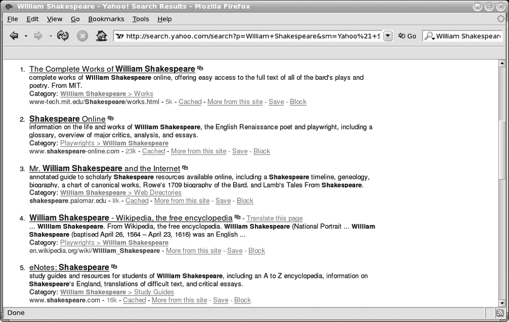
There is no need to visit any of these sites (which may be a pity): we have found our answer in the data returned from the search engine index itself. The fourth entry tells us that Shakespeare was born in 1564.

When an index is sufficiently loaded with information, going to the place it points to becomes unnecessary. This very same reasoning is at the root of an often used optimization tactic. We can improve the speed of a frequently run query by stuffing into an index additional columns (one or more) which of themselves have no part to play in the actual search criteria, but which crucially hold the data we need to answer our query. Thus the data that we require can be retrieved entirely from the index, cutting out completely the need to access the original source data. Some products such as DB2 are clever enough to let us specify that a unique index includes some other columns and check uniqueness of only a part of the composite key. The same result can be achieved with Oracle, in a somewhat more indirect fashion, by using a non-unique index to enforce a uniqueness or primary key constraint.

Conversely, there have been cases of batch programs suddenly taking much more time to run to completion than previously, following what appears to be the most insignificant modification to the query. This minor change was the addition of another column to the list of columns returned by a select statement. Unfortunately, prior to the modification, the entire query could be satisfied by reference to the data returned from an index. The addition of the new column forced the database to go back to the table, resulting in a hugely significant increase in processor activity.

Let’s look in more detail at the contrast between “index only” and “index plus table” retrieval performance. Figure 5-2 illustrates the performance impact of fetching one additional column absent from the index that is used to answer the query for three of the major database systems. The table used for the test was the same in all cases, having 12 columns populated with 250,000 rows. The primary key was defined as a three-column composite key, consisting of first an integer column with random values uniformly spread between 1 and 5,000, then a string of 8 to 10 characters, and then finally a datetime column. There is no other index on the table other than the unique index that implements the primary key. The reference query is fetching the second and third columns in the primary key on the basis of a random value of between 1 and 5,000 in the first column. The test measures the performance impact of fetching one more column—numeric and therefore relatively small—that doesn’t belong to the index. The results in Figure 5-2 are normalized such that the case of fetching two columns that are found in the index is always pegged at 100%. The case of having to go to the table and fetch an additional column absent from the index is then expressed as some percentage less than 100%.

Figure 5-2. Performance impact of fetching a third column that has to be retrieved from the table

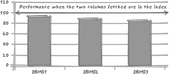
Figure 5-2 shows that the performance impact of having to go to the table as well as to the index isn’t enormous (around 5 or 10%) but nevertheless it is noticeable, and it is much more so with some database products than with others. As always, the exact numbers may vary with circumstances, and the impact can be much more severe if the table access requires additional physical I/O operations, which isn’t the case here.

Pushing to the extreme the principle of storing as much data as possible in the indexes, some database management systems, such as Oracle, allow you to store all of a table’s data into an index built on the primary key, thus getting rid of the table structure altogether. This approach saves storage and may save time. The table is the index, and is known as an index-organized table (I0T) as opposed to the regular heap structure.

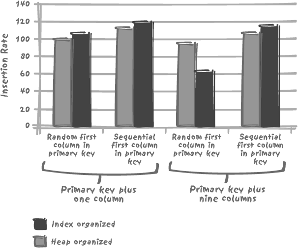
After the discussion in Chapter 3 about the cost penalty of index insertion, you might expect insertions into an index-organized table to be less costly than applying insertions to a table with no other index than the primary key enforcement index. In fact, in some circumstances the opposite is true, as you can see from Figure 5-3. It compares insertion rates for a regular table against those for an IOT. The tests used a total of four tables. Two table patterns with the same column definitions were created, once as a regular heap table, and once as an IOT. The first table pattern was a small table consisting of the primary key columns plus one additional column, and the second pattern a table consisting of the primary key columns plus nine other columns, all numeric. The (compound) primary key in every table was defined as a number column, a 10-character string, and a timestamp. For each case, two tests were performed. In the first test, the primary key was subjected to the insertion of randomly ordered primary key values. The second test involved the insertion into the leading primary key column of an increasing, ordered sequence of numbers.

Where the table holds few columns other than the ones that define the primary key, it is indeed faster to insert into an IOT. However, if the table has even a moderate number of columns, all those columns that don’t pertain to the primary key also have to be stored in the index structure (sometimes to an overflow area). Since the table is the index, much more information is stored there than would otherwise be the case. Chapter 3 has also shown that inserting into an index is intrinsically more costly than inserting into a regular table. The byte-shuffling cost associated with inserting more data into a more complicated structure can lead to a severe performance penalty, unless the rows are inserted in the same or near-the-same order as the primary key index. The penalty is even worse with long character strings. In many cases the additional cost of insertion outweighs the benefit of not having to go to the table when fetching data through the primary key index.^[*]

Figure 5-3. Relative cost of inserting into an Oracle index-organized table compared to a regular (heap-organized) table

There are, however, some other potential benefits linked to the strong internal ordering of indexes, as you shall see next.

There is another aspect to an index-organized table than just finding all required data in the index itself without requiring an additional access to the table. Because IOTs, being indexes, are, first and foremost, strongly ordered structures, their rows are internally ordered. Although the notion of order is totally foreign to the relational theory, from a practical point of view whenever a query refers to a range of values, it helps to find them together instead of having to gather data scattered all over the table. The most common example of this sort of application is range searching on time series data, when you are looking for events that occurred between two particular dates.

Most database systems manage to force such an ordering of rows by assigning to an index the role of defining the order of rows in the table. SQL Server and Sybase call such an index a clustered index . DB2 calls it a clustering index , and it has much the same effect in practice as an Oracle IOT. Some queries benefit greatly from this type of organization. But similar to index organized tables, updates to columns pertaining to the index that defines the order are obviously more costly because they entail a physical movement of the data to a new position corresponding to the “rank” of the new values. The ordering of rows inevitably favors one type of range-scan query at the expense of range scans on alternative criteria.

As with IOTs that are defined by the primary key, it is safer to use the primary key index as the clustering index, since primary keys are never updated (and if your application needs to update your primary key, there is something very seriously wrong indeed with your design, and it won’t take long before there is something seriously wrong with the integrity of your data). In contrast to IOTs, an index other than the one that enforces the primary key constraint can be chosen as the clustering index. But remember that any ordering unduly favors some processes at the expense of others. The primary key, if it is a natural key, has a logical significance; the associated index is more equal than all the other indexes that may be defined on the table, even unique ones. If some columns must be given some particular prominence through the physical implementation, these are the ones.

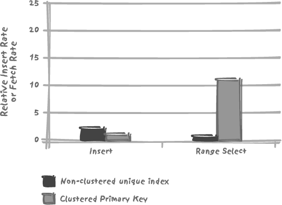
Figure 5-4 illustrates the kind of differences you may expect between clustered and non-clustered index performance in practice. If we take the same table as was used for the index-organized table in Figure 5-3’s example (a three-column primary key plus nine numeric columns), and if we insert rows in a totally random way, the cost of insertion into a table where the primary key index is clustered is quite high, since tests show that our insertion rate is about half the insertion rate obtained with a non-clustered primary key. But when we run a range scan test on about 50,000 rows, this clustered index provides really excellent performance. In this particular case, the clustered index allows us to outperform the non-clustered approach by a factor of 20. We should, of course, see no difference when fetching a single row.

A structural optimization, such as a clustered index or an IOT, necessarily has some drawbacks. For one thing, such structures apply some strong, tree-based, and therefore hierarchical ordering to tables. This approach resurrects many of the flaws that saw hierarchical databases replaced by relational databases in the corporate world. Any hierarchical structure favors one vision of the data and one access path over all the others. One particular access path will be better than anything you could get with a non-clustered table, but most other access paths are likely to be significantly worse. Updates may prove more costly. The initial tidy disposition of the data inside the database files may deteriorate faster at the physical level, due to chaining, overflow pages, and similar constructs, which take a heavy toll on performance. Clustered structures are excellent in

Figure 5-4. How clustered indexes perform

some cases, boosting performance by an impressive factor. But they always need to be carefully tested, because there is a high probability that they will make many other processes run slower. One must judge their suitability while looking at the global picture—and not on the basis of one particular query.

You have seen that finding all the rows together when doing a range scan can be highly beneficial to performance. There are, actually, other means to achieve a grouping of data than the somewhat constraining use of clustering indexes or index-organized tables. All database management systems let us partition tables and indexes—an application of the old principle of divide and rule. A large table may be split into more manageable chunks. Moreover, in terms of process architecture, partitioning allows an increased concurrency and parallelism, thus leading to more scalable architectures, as you shall see in Chapters 9 and 10.

First of all, beware that this very word, partition, has a different meaning depending on the DBMS under discussion, sometimes even depending on the version of the DBMS. There was a time, long ago, when what is now known as an Oracle tablespace used to be referred to as a partition.

Despite the fact that partitioning spreads data from a table over multiple, somewhat independent partitions, data-driven partitioning is not a panacea for resolving concurrency problems. For example, we might partition a table by date, having one partition per week of activity. Doing so is an efficient way to spread data for one year over 52 logically distinct areas. The problem is that during any given week everybody will rush to the same partition to insert new rows. Worse, if our partitioning key is the current system date and time, all concurrent sessions will be directed towards the very same data block (unless some structural implementation tricks have been introduced, such as maintaining several lists of pages or blocks where we can insert). As a result, we may have some very awkward memory contention. Our large table will become a predominantly cold area, with a very hot spot corresponding to most current data. Such partitioning is obviously less than ideal when many processes are inserting concurrently.

On the other hand, let’s assume that we choose to partition according to the geographical origin of a purchase order (we may have to carefully organize our partitioning if our products are more popular in some areas and suffer from heavier competition elsewhere). At any given moment, since sales are likely to come from nowhere in particular, our inserts will be more or less randomly spread over all our partitions. The performance impact from our partitioning will be quite noticeable when we are running geographical reports. Of course, because we have partitioned on spatial criteria, time-based reports will be less efficiently generated than if we had partitioned on time. Nevertheless, even time-based queries may, to some extent, benefit from partitioning since it is quite likely that on a multiprocessor box the various partitions will be searched in parallel and the subsequent results merged.

There are therefore two sides to partitioning. On the one hand, it is an excellent way to cluster data according to the partitioning key so as to achieve faster data retrieval. On the other hand, it is a no-less-excellent way to spread data during concurrent inserts so as to avoid hot spots in the table. These two objectives can work in opposition to one another, so the very first thing to consider when partitioning is to identify the major problem, and partition against that. But it is important to check that the gain on one side is not offset by the loss on the other. The ideal case is when the clustering of data for selects goes hand in hand with suitably spread inserts, but this is unfortunately not the most common situation.

You may be tempted to believe that if we have a very large table and want to avoid contention when many sessions are simultaneously writing to the database, then we are necessarily better off partitioning the data in one way or another. This is not always true.

Suppose that we have a large table storing the details of orders passed by our customers. If, as sometimes happens, a single customer represents the bulk of our activity, partitioning on the customer identifier is not going to help us very much. We can very roughly divide our queries into two families: queries relating to our big customer and queries relating to the other, smaller customers. When we query the data relating to one small customer, an index on the customer identifier will be very selective and therefore efficient, without any compelling need for partitioning. A clever optimizer fed with suitable statistics about the distribution of keys will be able to detect the skewness and use the index. There will be little benefit to having those small customers stored into smallish partitions next to the big partition holding our main customer.

Conversely, when querying the data attached to our major customer, the very same clever optimizer will understand that scanning the table is by far the most efficient way of proceeding. In that case, fully scanning a partition that comprises, for example, 80% of the total volume will not be much faster than doing a full table scan. The end users will hardly notice the performance advantage, whereas the purchasing department will most certainly notice the extra cost of the separately priced partitioning option.

Never forget that what dictates the choice of a nonstandard storage option such as partitioning is the global improvement of business operations. It may mean improving a business process that is perceived as being of paramount importance to the detriment of some other processes. For instance, it makes sense to optimize transactional processing that takes place during business hours at the expense of a nightly batch job that has ample time to complete. The opposite may also be true, and we may decide that we can afford to have very slightly less responsive transactions if it allows us to minimize a critical upload time during which data is unavailable to users. It’s a matter of balance.

In general, you should avoid unduly favoring one process over another that needs to be run under similar conditions. In this regard, any type of storage that positions data at different locations based on the data value (for example both clustering indexes as well as partitioning) are very costly when that value is updated. What would have previously been an in situ update in a regular table, requiring hardly more than perhaps changing and shifting a few bytes in the table at an invariant physical address, becomes a delete on one part of the disk, followed by an insert somewhere else, with all the maintenance operations usually associated with indexes for this type of operation.

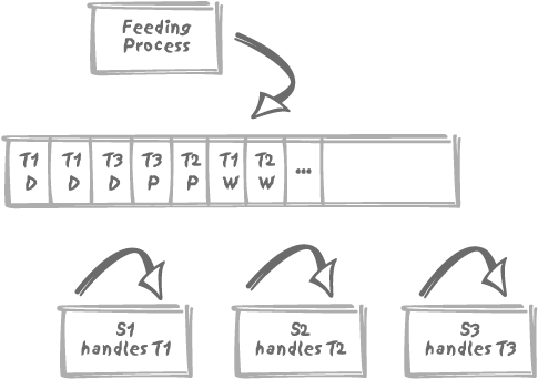
Having to move data when we update partition keys seems, on the surface, to be a situation best avoided. Strangely, however, partitioning on a key that is updated may sometimes be preferable to partitioning on a key that is immutable once it has been inserted. For example, suppose that we have a table being used as a service queue. Some process inserts service requests into this table that are of different types (say type T₁ to type T_n). New service requests are initially set to status W, meaning “waiting to be processed.” Server processes S₁ to S_p regularly poll the table for requests with the W status, change the status of those requests to P (meaning “being processed”), and then, as each request is completed its status is set to D for “done.”

Let’s further suppose that we have as many server processes as we have request types, and that each server process is dedicated to handling a particular type of request. Figure 5-5 shows the service queue as well as the processes. Of course, since we cannot let the table fill with “done” requests, there must be some garbage-collecting process, not shown, that removes processed requests after a suitable delay.

Figure 5-5. A service queue

Each server process regularly executes a select (actually, a select ... for update) query with two criteria, the type, which depends on the server, and a condition:

    and status = 'W'

Let’s consider alternative ways of partitioning the service queue table. One way to partition the table, and possibly the most obvious, is to partition by request type. There is a big advantage here should any server process crash or fall behind in one way or another. The queue will lengthen for that process until it finally catches up, but the interruption to the processing of that queue will have no influence on the other processes.

Another advantage of partitioning by request type is that we avoid having requests of any one type swamp the system. Without partitioning, the polling processes scan a queue that under normal circumstances contains very few rows of interest. If we have a common waiting line and all of a sudden we have a large number of requests of one type and status, all the processes will have more requests to inspect and therefore each will be slowed down. If we partition by type, we establish a watertight wall between the processing of different types.

But there is another possible way to partition our service queue table, and that is by status. The downside is obvious: any status change will make a request migrate from one partition to the next. Can there be any advantage to such migration? Actually, there may indeed be benefit in this approach. Everything in partition W is ready and waiting to be processed. So there is no need to scan over requests being processed by another server or requests that have already been processed. Therefore, the cost of polling may be significantly reduced. Another advantage is that garbage collection will operate on a separate partition, and will not disturb the servers.

We cannot say definitively that “partitioning must be by type” or “partitioning must be by status.” It depends on how many servers we have, their polling frequency, the relative rate at which data arrives, the processing time for each type of request, and how often we remove processed requests, and so on. We must carefully test various hypotheses and consider the overall picture. But it is sometimes more efficient for the overall system to sacrifice outright performance for one particular operation, if by doing so other, more frequently running processes are able to obtain a net advantage, thus benefiting the global business operations.

We have seen that physically grouping rows together is of most benefit when performing range scans, where we are obviously interested in a succession of logically adjacent rows. But our discussion so far has been with regard to retrieving data from only one table. Unless the database design is very, very, very bad, most queries will involve far more than one table. It may therefore seem somewhat questionable if we group all the data from one table into one physical location, only to have to complete the retrieval by visiting several randomly scattered locations for data from a second and subsequent tables. We need some method to group data from at least two tables into the same physical location on disk.

The answer lies in pre-joined tables, a technique that is supported by some database systems. Pre-joining is not the same as summary tables or materialized views, which are themselves nothing other than redundant data, pre-digested results that are updated more or less automatically.

Pre-joined tables are tables that are physically stored together, based on some criterion that will usually be the join condition. (Oracle calls such a set of pre-joined tables a cluster, which has nothing to do with either index clustering, as defined earlier in this chapter, nor with the MySQL clusters of databases, which are multiple servers accessing the same set of tables.)

When tables are pre-joined, the basic unit of storage (a page or a block), normally devoted to the data from a single table, holds data from two or more tables, brought together on the basis of a common join key. This arrangement may be very efficient for one specific join. But it often proves to be a disaster for everything else. Here’s a review of some of the disadvantages of pre-joining tables:

This particular type of storage should be used extremely sparingly to solve very specific issues, and then only by database administrators. Developers should forget about this technique.

It is reasonable and safe to assume that any storage option that is not the default one, however attractive it may look, can introduce a degree of complexity out of all proportion to the possible gains that may (or may not) be achieved. In the worst case, a poorly chosen storage option can dramatically degrade performance. Military history is full of impregnable fortresses built in completely the wrong places that failed to fill any useful purpose, and of many a Great Wall that never prevented any invasion because the enemy, a bad sport, failed to behave as planned. All organizations undergo changes, such as divisions and mergers. Business plans and processes may change, too. Careful plans may have to be scrapped and rebuilt from scratch.

The trouble with structuring data in a particular way is that it is often done with a particular type of process in mind. One of the beauties of the relational model is its flexibility. By strongly structuring your data at the physical level, you may sacrifice, in a somewhat hidden way, some of this flexibility. Of course, some structures are less constraining than others, and data partitioning is almost unavoidable with enormous databases. But always test very carefully and keep in mind that changing the physical structure of a big database because it was poorly done initially can take days, if not weeks, to complete.