Even before starting to write the very first SQL statement in a program, you should have an idea about the search criteria that will be of importance to users. Values that are fed into a program and the size of the data subset defined lay the foundations for indexing. Indexes are, above all, a technique for achieving the fastest possible access to specific data. Note that I say “specific data,” as indexes must be carefully deployed. They are not a panacea: they will not enable fast access to all data. In fact, sometimes the very opposite is the result, if there is a serious mismatch between the original index strategy and the new data-retrieval requirements.

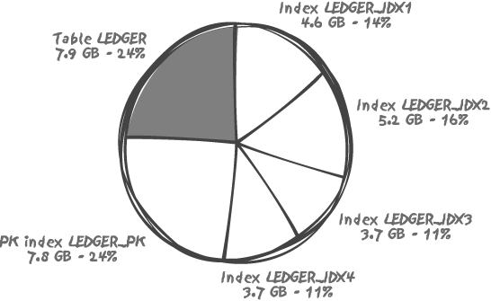
Indexes can be considered to be shortcuts to data, but they are not shortcuts in the same sense as a shortcut in a graphical desktop environment. Indexes come with some heavy costs, both in terms of disk space and, possibly more importantly, in terms of processing costs. For example, it is not uncommon to encounter tables in which the volume of index data is much larger than the volume of the actual data being indexed. I can say the same of index data as I said of redundant table data in Chapter 1: indexes are usually mirrored, backed up to other disks, and so on, and the very large volumes involved cost a lot, not only in terms of storage, but also in terms of downtime when you have to restore from a backup.

Figure 3-1 shows a real-life case, the main accounting table of a major bank; out of 33 GB total for all indexes and the table, indexes take more than 75%.

Let’s forget about storage for a moment and consider processing. Whenever we insert or delete a row, all the indexes on the table have to be adjusted to reflect the new data. This adjustment, or “maintenance,” also applies whenever we update an indexed column; for example, if we change the value of an attribute in a column that is either itself indexed, or is part of a compound index in which more than one column is indexed together. In practice this maintenance activity means a lot of CPU resources are used to scan data blocks in memory, I/O activity is needed to record the changes to logfiles, together with possibly more I/O work against the database files. Finally, recursive operations may be required on the database system to maintain storage allocations.

Figure 3-1. A real-life case: Data versus Index out of a 33 GB total

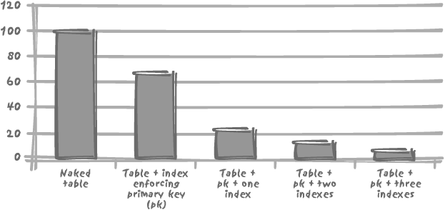
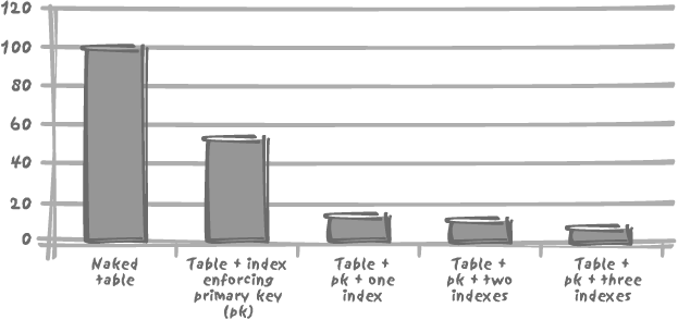
Tests have quantified the real cost of maintaining indexes on a table. For example, if the unit time required to insert data into a non-indexed table is 100 (seconds, minutes, or hours—it does not really matter for this illustration), each additional index on that table will add an additional unit time of anything from 100 to 250.

Although index implementation varies from DBMS to DBMS, the high cost of index maintenance is true for all products, as Figures 3-2 and 3-3 show with Oracle and MySQL.

Figure 3-2. The impact of indexes on insertion with Oracle

Figure 3-3. The impact of indexes on insertion with MySQL

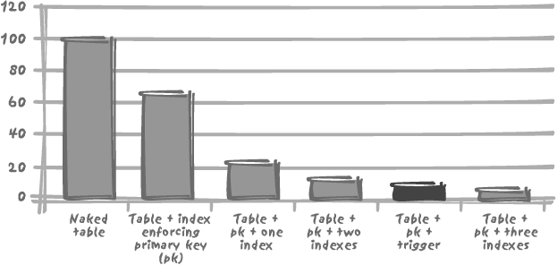
Interestingly, this index maintenance overhead is of the same magnitude as a simple trigger. I have created a simple trigger to record into a log table the key of each row inserted together with the name of the user and a timestamp—a typical audit trail. As one might expect, performance suffers—but in the same order of magnitude as the addition of two indexes, as shown in Figure 3-4. Recall how often one is urged to avoid triggers for performance reasons! People are usually more reluctant to use triggers than they are to use indexes, yet the impact may well be very similar.

Figure 3-4. Comparing the performance impact of indexes and triggers

Generating more work isn’t the only way for indexes to hinder performance. In an environment with heavy concurrent accesses, more indexes will mean aggrieved contention and locking. By nature, an index is usually a more compact structure than a table—just compare the number of index pages in this book to the number of pages in the book itself. Remember that updating an indexed table requires two data activities: updating the data itself and updating the index data. As a result, concurrent updates, which may affect relatively scattered areas of a huge table, and therefore not suffer from any serialization during the changes to the actual data, may easily find themselves with much less elbow room when updating the indexes. As explained above, these indexes are by definition much “tighter” data assemblages.

It must be stressed that, whatever the cost in terms of storage and processing power, indexes are vital components of databases. Their importance is nowhere greater, as I discuss in Chapter 6, than in transactional databases where most SQL statements must either return or operate on few rows in large tables. Chapter 10 shows that decision support systems are also heavily dependent for performance on indexing. However, if the data tables we are dealing with have been properly normalized (and once again I make no apologies for referring to the importance of design), those columns deserving some a priori indexing will be very few in a transactional database. They will of course include the primary key (the tuple, or row, identifier). This column (or columns in the case of a compound key) will be automatically indexed simply by virtue of its declaration as the primary key. Unique columns are similar and will, in all probability, be indexed simply as a by-product of the implementation of integrity constraints. Consideration should also be given to indexing columns that, although not unique, approach uniqueness—in other words, columns with a high variability of values.

As a general rule, experience would suggest that very few indexes are required for most tables in a general purpose or transactional database, because many tables are searched with a very limited set of criteria. The rationale may be very different in decision support systems, as you shall see in Chapter 10. I tend to grow suspicious of tables with many indexes, especially when these tables are very large and much updated. A high number of indexes may exceptionally be justified, but one should revisit the original design to validate the case for heavily indexed tables.

The book metaphor can be helpful in another respect—as a means of better understanding the role of the index in the DBMS. It is important to recognize the distinction between the two mechanisms of the table of contents and the book index. Both provide a means of fast access into the data, but at two very different levels of granularity. The table of contents provides a structured overview of the whole book. As such, it is regarded as complementary to the index device in books, which is often compared to the index of a database.

When you look for a very precise bit of information in a book, you turn to the index. You are ready to check 2 or 3 entries, but not 20--flipping pages between the index and the book itself to check so many entries would be both tedious and inefficient. Like a book index, a database index will direct you to specific values in one or more records (I overlook the use of indexes in range searching for the moment).

If you look for substantial information in a book, you either turn to the index, get the first index entry about the topic you want to study, and then read on, or you turn to the table of contents and identify the chapter that is most relevant to your topic. The distinction between the table of contents and the index is crucial: an entry in a table of contents directs the reader to a block of text, perhaps a chapter, or a section. Similarly, Chapter 5 shows mechanisms by which you can organize a table and enable data retrieval in a manner similar to a table of contents’ access.

An index must primarily be regarded as a means of accessing data at an atomic level of granularity, as defined by the original data design, and not as a means of retrieving large quantities of undifferentiated data. When an indexing strategy is used to pull in large quantities of data, the role of indexes is being seriously misunderstood. Indexing is being used as a desperate measure to recover from an already untenable situation. The commander is beginning to panic and is sending off sorties in all directions, hoping that sheer numbers will compensate for the lack of a coherent strategy. It never does, of course.

To justify the use of an index, it must provide benefit. Just as in our metaphor of the book, you may use an index if you simply require very particular information on one item of data. But if you want to review an entire subject area, you will turn not to the index, but to the table of contents of the book.

There will always be times when the decision between using an index or a broader categorization is a difficult one. This is an area where the use of retrieval ratios makes its persuasive appearance. Such ratios have a hypnotic attraction to many IT and data practitioners because they are so neat, so easy, so very scientific!

The applicability of an index has long been judged on the percentage of the total data retrieved by a query that uses a key value as only search criterion, and conventionally that percentage has often been set at 10% (the percentage of rows that match, on average, an index key defines the selectivity of the index; the lower the percentage, the more selective the index). You will often find this kind of rule in the literature. This ratio, and others like it, is based on old assumptions regarding such things as the relative performance of disk access and memory access. Even if we forget that these performance ratios, which have been around since at least the mid-1980s, were based on what is today outdated technology (ideal percentages are grossly simplistic views), far more factors need to be taken into account.

When magical ratios such as our 10% ratio were designed, a 500,000-row table was considered a very big table; 10% of such a table usually meant a few tens of thousand rows. When you have tables with hundreds of millions or even billions of rows, the number of rows returned by using an index with a similar selectivity of about 10% may easily be greater than the number of rows in those mega-tables of yore against which the original ratios were estimated.

Consider the part played by modern hard disk systems, equipped as they are with large cache storage. What the DBMS sees as “physical I/O” may well be memory access; moreover, since the kernel usually shifts different amounts of data into memory depending on the type of access (table or index), you may be in for a surprise when comparing the relative performance of retrievals with and without using an index. But these are not the only factors to consider. You also need to watch the number of operations, which can truly be performed in parallel. Take note of whether the rows associated with an index key value are likely to be physically close. For instance, when you have an index on the insertion date, barring any quirk such as the special storage options I describe in Chapter 5, any query on a range of insertion dates will probably find the corresponding rows grouped together by construction. Any block or page pointed to by the very first key in the range will probably contain as well the rows pointed to by the immediately following key values. Therefore, any chunk of table we return through use of the index will be rich in data of interest to our query, and any data block found through the index will be of considerable value to the query’s performance.

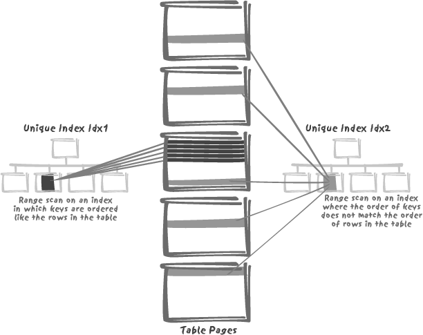
When the indexed rows associated with an index key are spread all over the table (for example, the references to an article in a table of orders), it is quite another matter. Even though the number of relevant rows is small as a proportion of the whole, because they are scattered all over the disk, the value of the index diminishes. This is illustrated by Figure 3-5: we can have two unique indexes that are strictly equivalent for fetching a single row, and yet one will perform significantly better than the other if we look for a range of values, a frequent occurrence when working with dates.

Factors such as these blur the picture, and make it difficult to give a prescriptive statement on the use of indexes.

Figure 3-5. When two highly selective indexes may perform differently

Indexes are usually implemented as tree structures—mostly complex trees—to avoid a fast decay of indexes on heavily inserted, updated, and deleted tables. To find the physical location of a row, the address of which is stored in the index, one must compare the key value to the value stored in the current node of the tree to be able to determine which sub-tree must be recursively searched. Let’s now suppose that the value that drives our search doesn’t exactly match an actual column value but can be compared to the result of a function f( ) applied to the column value. In that case we may be tempted to express a condition as follows:

    where f(indexed_column) = 'some value'

This kind of condition will typically torpedo the index, making it useless. The problem is that nothing guarantees that the function f( ) will keep the same order as the index data; in fact, in most cases it will not. For instance, let’s suppose that our tree-index looks like Figure 3-6.

Figure 3-6. A simplistic representation of how names might be stored in an index

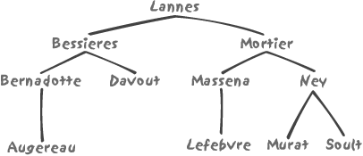
(If the names look familiar, it is because they are those of some of Napoleon’s marshals.) Figure 3-6 is of course an outrageously simplified representation, just for the purpose of explaining a particular point; the actual indexes do not look exactly like the binary tree shown in Figure 3-6. If we look for the MASSENA key, with this search condition:

    where name = 'MASSENA'

then the index search is simple enough. We hit LANNES at the root of the tree and compare MASSENA to LANNES. We find MASSENA to be greater, based on the alphabetical order. We therefore recursively search the right-hand sub-tree, the root of which is MORTIER. Our search key is smaller than MORTIER, so we search the left-hand sub-tree and immediately hit MASSENA. Bingo—success.

Now, let’s say that we have a condition such as:

    where substr(name, 3, 1) = 'R'

The third letter is an uppercase R--which should return BERNADOTTE, MORTIER, and MURAT. When we make the first visit to the index, we hit LANNES, which doesn’t satisfy the condition. Not only that, the value that is associated with the current tree node gives us no indication whatsoever as to which branch we should continue our search into. We are at a loss: the fact that the third letter is R is of no help in deciding whether we should search the left sub-tree or the right sub-tree (in fact, we find elements belonging to our result set in both sub-trees), and we are unable to descend the tree in the usual way, by selecting a branch thanks to the comparison of the search key to the value stored in the current node.

Given the index represented in Figure 3-6, selecting names with an R in the third position is going to require a sequential data scan, but here another question arises. If the optimizer is sufficiently sophisticated, it may be able to judge whether the most efficient execution path is a scan of the actual data table or inspecting, in turn, each and every node in the index on the column in question. In the latter case, the search would lead to an index-based retrieval, but not as envisaged in the original model design since we would be using the index in a rather inefficient way.

Recall the discussion on atomicity in Chapter 1. Our performance issue stems from a very simple fact: if we need to apply a function to a column, it means that the atomicity of data in the table isn’t suitable for our business requirements. We are not in 1NF!

Atomicity, though, isn’t a simple notion. The ultra-classic example is a search condition on dates. Oracle, for instance, uses the date type to store not only the date information, but also the time information , down to the second (this type is actually known as datetime to most other database systems). However, to test the unwary, the default date format doesn’t display the time information. If you enter something such as:

    where date_entered = to_date('18-JUN-1815',
                                 'DD-MON-YYYY')

then only the rows for which the date (and time!) happens to be exactly the 18th of June 1815 at 00:00 (i.e., at midnight) are returned. Everyone gets caught out by this issue the very first time that they query datetime data. Quite naturally, the first impulse is to suppress the time information from date_entered, which the junior practitioners usually do in the following way:

    where trunc(date_entered) = to_date('18-JUN-1815',
                                        'DD-MON-YYYY')

Despite the joy of seeing the query “work,” many people fail to realize (before the first performance issues begin to arise) that by writing their query in such a way they have waved goodbye to using the index on date_entered, assuming there was one. Does all this mean that you cannot be in 1NF if you are using datetime columns? Fortunately, no. In Chapter 1, I defined an atomic attribute as an attribute in which a where clause can always be referred to in full. You can refer in full to a date if you are using a range condition. An index on date_entered is usable if the preceding condition is written as:

    where date_entered >= to_date('18-JUN-1815',
                                     'DD-MON-YYYY')
      and date_entered < to_date('19-JUN-1815',
                                    'DD-MON-YYYY')

Finding rows with a given date in this way makes an index on date_entered usable, because the very first condition allows us to descend the tree and reach a sorted list of all keys at the bottom of the index hierarchy (we may envision the index as a sorted list of keys and associated addresses, above which is plugged a tree allowing us to get direct access to every item in the list). Therefore, once the first condition has taken us to the bottom layer of the index and to the very first item of interest in the list, all we have to do is scan the list as long as the second condition is true. This type of access is known as an index range scan .

The trap of functions preventing the use of indexes is often even worse if the DBMS engine is able to perform implicit conversions when a column of a given type is equated or compared to a constant of another type in a where condition—a logical error and yet one that is allowed by SQL. Once again Oracle provides an excellent example of such behavior. For instance, dangers arise when a character column is compared to a number. Instead of immediately generating a run-time error, Oracle implicitly converts the column to a number to enable the comparison to take place. The conversion may indeed generate a run-time error if there is an alpha character in that numerical string, but in many cases when a string of digits without any true numerical meaning is stored as characters (social security numbers or a date of birth shown as mmddyy, or ddmmyy, both meaning the same, but having very different numerical values), the conversion and subsequent comparison will “work"--except that the conversion will have rendered any index on the character column almost useless.

In the light of the neutralization of indexes by functions, Oracle’s design choice to apply the conversion to the column rather than to the constant may at first look surprising. However, that decision does make some sense. First of all, comparing potatoes to carrots is a logical error. By applying the conversion to the column, the DBMS is more likely (depending on the execution path) to encounter a value to which the conversion does not apply, and therefore the DBMS is more likely to generate a runtime error. An error at this stage of the process will prove a healthy reminder to the developer, doubtless prompting for a correction in the actual data field and raising agonizing questions about the quality of the data. Second, assuming that no error is generated, the very last thing we want is to return incorrect information. If we encounter:

    where account_number = 12345

it is quite possible, and in fact most likely, that the person who wrote the query was expecting the account 0000012345 to be returned—which will be the case if account_number (the alpha string) is converted to number, but not if the query 12345 is converted to a string without any special format specification.

One may think that implicit conversions are a rare occurrence, akin to bugs. There is much truth in the latter point, but implicit conversions are in fact pretty common, especially when such things come into play as a parameters table holding in a column named parameter_value string representations of numbers and dates, as well as filenames or any other regular character string. Always make conversions explicit by using conversion functions.

It is sometimes possible to index the result of a function applied to one or more columns. This facility is available with most products under various names (functional index, function-based index, index extension, and so on, or, more simply, index on a computed column). In my view, one should be careful with this type of feature and use it only as a standby for those cases in which the code cannot be modified.

I have already mentioned the heavy overhead added to data modifications as a result of the presence of indexes. Calling a function in addition to the normal index load each time an index needs to be modified cannot improve the situation: indeed it only adds to the total index maintenance cost. As the date_entered example given earlier demonstrates, creating a function-based index may be the lazy solution to something that can easily be remedied by writing the query in a different way. Furthermore, nothing guarantees that a function applied to a column retains the same degree of precision that a query against the raw column will achieve. Suppose that we store five years of sales online and that the sales_date column is indexed. On the face of it, such an index looks like an efficient one. But indexing with a function that is the month part of the date is not necessarily very selective, especially if every year the bulk of sales occurs in the run up to Christmas. Evaluating whether the resulting functional index will really bring any benefit is not necessarily easy without very careful study.

From a purely design point of view, one can argue that a function is an implicit recognition that the column in question may be storing two or more discrete items of data. Use of a functional index is, in most cases, a way to extract some part of the data from a column. As pointed out earlier, we are violating the famous first normal form, which requires data to be “atomic.” Not using strictly “atomic” data in the select list is a forgivable sin. Repeatedly using “subatomic” search criteria is a deadly one.

There are some cases, though, when a function-based index may be justified. Case-insensitive searches are probably the best example; indexing a column converted to upper- or lowercase will allow us to perform case-insensitive searches on that column efficiently. That said, forcing the case during inserts and updates is not a bad solution either. In any event, if data is stored in lowercase, then required in uppercase, one has to question the thoroughness with which the original data design was carried out.

Another tricky conundrum is the matter of duration in the absence of a dedicated interval data type. Given three time fields, a start date, a completion date, and a duration, one value can be determined from any existing two—but only by either building a functional index or by storing redundant data. Whichever solution is followed, redundancy will be the inevitable consequence: in the final analysis, you must weigh the benefits and disadvantages of the issues surrounding function-based indexes so that you can make informed decisions about using them.

It is quite customary to systematically index the foreign keys of a table; and it is widely acknowledged to be common wisdom to do so. In fact, some design tools automatically generate indexes on these keys, and so do some DBMS. However, I urge caution in this respect. Given the overall cost of indexes, unnecessarily indexing foreign keys may prove a mistake, especially for a table that has many foreign keys.

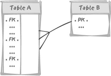
The rule of indexing the foreign keys comes from what happens when (for example) a foreign key in table A references the primary key in table B, and then both tables are concurrently modified. The simple model in Figure 3-7 illustrates this point.

Figure 3-7. The simple, Master-Detail example

Imagine that table A is very large. If user U1 wants to remove a row from table B, since the primary key for B is referenced by a foreign key in A, the DBMS must check that removal of the row will not lead to inconsistencies in the intertable dependencies, and must therefore see whether there is any child row in A referencing the row about to be deleted from B. If there does happen to be a row in A that references our row in B, then the deletion must fail, because otherwise we would end up with an orphaned row and inconsistent data. If the foreign key in A is indexed, it can be checked very quickly. If it is not indexed, it will take a significant period of time since the session of user U1 will have to scan all of table A.

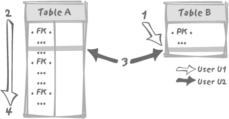
Another problem is that we are not supposed to be alone on this database, and lots of things can happen while we scan A. For instance, just after user U1 has started the hunt in table A for an hypothetical child row, somebody else, say user U2, may want to insert a new row into table A which references that very same row we want to delete from table B. This situation is described in Figure 3-8, with user U1 first accessing table B to check the identifier of the row it wants to delete (1), and then searching for a child in table A (2). Meanwhile, U2 will have to check that the parent row exists in table B. But we have a primary key index on B, which means that unlike user U1, who is condemned to a slow sequential scan of the foreign key values of table A, user U2 will get the answer immediately from table B. If U2 quietly inserts the new row in table A (3), U2 may commit the change at such a point that user U1 finishes checking and wrongly concludes, having found no row, that the path is clear for the delete.

Figure 3-8. Fight for the primary key

Locking is required to prevent such a case, which would otherwise irremediably lead to inconsistent data. Data integrity is, as it should be, one of the prime concerns of an enterprise-grade DBMS. It will take no chance. Whenever we want to delete a row from table B, we must prevent insertion into any table that references B of a row referencing that particular one while we look for child rows. We have two ways to prevent insertions into referencing tables (there may be several ones) such as table A:

In any case, if foreign keys are not indexed, checking for child rows will be slow, and we will hold locks for a very long time, potentially blocking many changes. In the worst case of the heavy-handed approach we can even encounter deadlocks, with two processes holding locks and stubbornly refusing to release them as long as the other process doesn’t release its lock first. In such a case, the DBMS usually solves the dispute by killing one of the processes (hasta la vista, baby...) to let the other one proceed.

The case of concurrent updates therefore truly requires indexing foreign keys to prevent sessions from locking objects much longer than necessary. Hence the oft heard rule that “foreign keys should always be indexed.” The benefit of indexing the foreign key is that the elapsed time for each process can be drastically reduced, and in turn locking is reduced to the minimum level required for ensuring data integrity.

What people often forget is that “always index foreign keys” is a rule associated with a special case. Interestingly, that special case often arises from design quirks, such as the maintenance of summary or aggregate denormalized columns in the master table of a master/detail relationship. There may be excellent reasons for updating concurrently two tables linked by referential integrity constraints. But there are also many cases with transactional databases where the referenced table is a “true” reference table (e.g., a dictionary, or “look-up” table that is very rarely updated, or it’s updated in the middle of the night when there is no other activity). In such a case, the only justification for the creation of an index on the foreign key columns should be whether such an index would be of any benefit from a strictly performance standpoint. We mustn’t forget the heavy penalty performance imposed by index maintenance. There are many cases when an index on a foreign key is not required.

The systematic indexing of foreign keys can often lead to situations in which columns belong to several indexes. Let’s consider once again a classic example. This consists of an ordering system in which some order_details table contains, for each order (identified by an order_id, a foreign key referencing the orders table) articles (identified by article_id, a foreign key referencing the articles table) that have been purchased, and in what quantity. What we have here is an associative table (order_details) resolving a many-to-many relationship between the tables orders and articles. Figure 3-9 illustrates the relationships among the three tables.

Figure 3-9. The Orders/Articles example

Typically, the primary key of order_details will be a composite key, made of the two foreign keys. Order entry is the very case when the referenced table and the referencing table are likely to be concurrently modified, and therefore we must index the order_id foreign key. However, the column that is defined here as a foreign key is already indexed as part of the composite primary key, and (this is the important point) as the very first column in the primary key. Since this column is the first column of the composite primary key, it can for all intents and purposes provide all the benefits as if it were an indexed foreign key. A composite index is perfectly usable even if not all columns in the key are specified, as long as those at the beginning of the key are.

When descending an index tree such as the one described earlier in this chapter, it is quite sufficient to be able to compare the leading characters of the key to the index nodes to determine which branch of the index the search should continue down. There is therefore no reason to index order_id alone, since the DBMS will be able to use the index on (order_id, article_id) to check for child rows when somebody is working on the orders table. Locks will therefore not be required for both tables. Note, once again, that this reasoning applies only because order_id happens to be the very first column in the composite primary key. Had the primary key been defined as (article_id, order_id), then we would have had to create an index on order_id alone, while not building an index on the other foreign key, article_id.

System-generated keys (whether through a special number column defined as self-incrementing or through the use of system-generated counters such as Oracle’s sequences) require special care. Some inexperienced designers just love system-generated keys even when they have perfectly valid natural identifiers at their disposal. System-generated sequential numbers are certainly a far better solution than looking for the greatest current value and incrementing it by one (a certain recipe for generating duplicates in an environment with some degree of concurrency), or storing a “next value” that has to be locked and updated into a dedicated table (a mechanism that serializes and dramatically slows down accesses). Nevertheless, when many concurrent insertions are running against the same table in which these automatic keys are being generated, some very serious contention can occur at the creation point of the primary key index level. The purpose of the primary key index is primarily to ensure the uniqueness of the primary key columns.

The problem is usually that if there is one unique generator (as opposed to as many generators as there are concurrent processes, hitting totally disjoint ranges of values) we are going to rapidly generate numbers that are in close proximity to each other. As a result, when trying to insert key values into the primary key index, all processes are going to converge on the same index page, and the DBMS engine will have to serialize—through locks, latches, semaphores, or whichever locking mechanism is at its disposal—the various processes so that each one does not try to overwrite the bytes that another one is writing to. This is a typical example of contention that leads to some severe underuse of the hardware. Processes that could and should work in parallel have to wait in order, one behind the other. This bottleneck can be particularly severe on multi-processor machines, the very environment in which parallelism should be operating.

Some database systems provide some means to reduce the impact of system-generated keys; for instance, Oracle allows you to define reverse indexes, indexes in which the sequence of bits making up the key is inversed before being stored into the index. To indicate a very approximate idea of what such an index looks like, let’s simply take the same names of marshals as we did in Figure 3-5 and reverse the letters instead of bits. We get something looking like Figure 3-10.

Figure 3-10. A simplified representation of reverse indexing

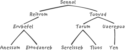
It is easy to understand that even when we insert names that are alphabetically very close to one another, they are spread all over the various branches of the index tree: look for instance at the respective positions of MASSENA (a.k.a. ANESSAM), MORTIER (REITROM) and MURAT (TARUM). Therefore, we hit different places in the index and have much less contention than with a normally organized index. Close grouping of the index values would lead to a very high write activity that is very localized within the index. Before searching, Oracle simply applies the same reversing to the value we want to search against, and then proceeds as usual to traverse the index tree.

Of course, every silver lining has its cloud: when our search condition attempts to use a leading string search like this:

    where name like 'M%'

which is a typical range search, the reverse index is no help at all. By contrast, a regular index can be used to quickly identify the range of values beginning with a certain string that we are interested in. The inability of reverse indexes to be used for range searches is, of course, a very minor inconvenience with system-generated keys, which are often unknown to end users and therefore unlikely to be the object of range scans. But it becomes a major hindrance when rows contain timestamps. Timestamped rows might arrive in close succession, making the timestamp column a potentially good candidate for reverse indexing, but then a timestamp is also the type of column against which we are quite likely to be looking for ranges of values.

The hash index used in some database systems represents a different way to avoid bottlenecking index updates all on one index page. With hash indexing, the actual key is transformed into a meaningless, randomly distributed numeric key generated by the system, which is based on the column value being indexed. Although it is not impossible for two values to be transformed into similar, meaningless keys, two originally “close” keys will normally hash into two totally disconnected values. Once again, hash indexes represent a trick to avoid having a hot spot inside an index tree, but that benefit too, comes with certain restrictions. The use of a hash index is on an “equality or nothing” basis; in other words, range searching, or indeed any query against a part of the index key, is out of the question. Nevertheless, direct access based on one particular value of the key can be very fast.

Even when there are solutions to alleviate contention risks, you should not create too many system-generated identifiers. I have sometimes found system-generated keys in each and every table (for instance a special, single detail_id for the type of order_details table mentioned above, instead of the more natural combination of order_id and some sequential number within the order). This blunderbuss approach is something that, by any standard, simply cannot be justified—especially for tables that are referenced by no other table.

It is very common to believe that if indexes are used in a query, then everything is fine. This is a gross misconception: there are many different characteristics of index access. Obviously, the most efficient type of index access is through a unique index, in which, at most, one row matches a given search value. Typically, such a search operation might be based on the primary key. However, as you saw in Chapter 2, accessing a table through its primary key may be very bad—if you are looping on all key values. Such an approach would be like using a teaspoon to move a big heap of sand instead of the big shovel of a full scan. So, at the tactical level, the most efficient index access is through a unique index, but the wider picture may reveal that this could be a costly mistake.

When several rows may match a single key value in a non-unique index (or when we search on a range of distinct values against a unique index), then we enter the world of range scanning. In this situation, we may retrieve a series of row addresses from the index, all containing the key values we are looking for. It may be a near-unique index, in which all key values match one row with the exception of a handful of values that match very few rows. Or it may be the other extreme of the non-unique indexed column for which all rows contain the same value. Indexed columns in which all rows contain the same value are in fact something you occasionally find with off-the-shelf software packages in which most columns are indexed, just in case. Never forget that finding the row in the index is all the work that is required only if:

In all other cases, we are only halfway to meeting the query requirement, and we must now access each data block (or page) by the address that is provided by the search of the index. Once again, all other things being equal, we may have widely different performance, depending on whether we shall find the rows matching our search value lumped together in the same area of the disk, or scattered all over the place.

The preceding description applies to the “regular” index accesses. However, a clever query optimizer may decide to use indexes in another way. It could operate on several indexes, combining them and doing some kind of pre-filtering before fetching the rows. It may decide to execute a full scan of a particular index, a strategy based on the judgment that this is the most efficient of all available methods for this particular query (we won’t go into the subtleties of what “most efficient” means here). The query optimizer may decide to systematically collect row addresses from an index, without taking the trouble to descend the index tree.

So, any reference to an index in an execution plan is far from meaning that “all’s well that runs well.” Some index accesses may indeed be very fast—and some desperately slow. Even a fast access in a query is no guarantee that by combining the query with another one, we could have got the result even faster. In addition, if the optimizer is indeed smart enough to ignore a useless index in queries, that same useless index will nevertheless require to be maintained whenever the table contents are modified. This index maintenance is something that may be especially significant in the massive uploads or purges routinely performed by a batch program. Useful or useless, an index has to be maintained.