
Chapter 15. Performance
- Type hints
- Transients
- Chunked sequences
- Memoization
- Understanding coercion
- Reducibles
Now that you’ve spent a book’s worth of material learning the why and how of Clojure, it’s high time we turned our attention to the subject of performance. There’s a meme in programming that can be summarized as follows: make it work first, and then make it fast. Throughout this book, we’ve taught you the ways Clojure allows you to “make it work,” and now we’re going to tell you how to “make it fast.”
In many cases, Clojure’s compiler can highly optimize idiomatic Clojure source code. But there are times when the form of your functions, especially in interoperability scenarios, will prove to be ambiguous or even counter to compiler optimizations. Therefore, we’ll lead you through optimization techniques such as type hints, transients, chunked sequences, memoization, and coercion. Using a combination of these techniques will help you approach, and sometimes exceed, the performance of Java.
The most obvious place to start, and the one you’re most likely to encounter, is type hinting—so this is where we’ll begin.
15.1. Type hints
The path of least resistance in Clojure often produces the fastest and most efficient compiled code, but not always. The beauty of Clojure is that this path of least resistance allows you to use simple techniques to gain speed via type hints. The first thing to know about type hints is that they’re used to indicate that an object is an instance of some class—never a primitive.
The Rule of Type Hinting
Write your code so it’s first and foremost correct; then add type-hint adornment to gain speed. Don’t trade the efficiency of the program for the efficiency of the programmer.
15.1.1. Advantages of type adornment
There are epic debates about the virtues of static versus dynamic type systems; we won’t engage in those arguments here. Instead we’ll note that Clojure provides the advantages of a dynamic type system but also allows type hinting after development, to mitigate some of the performance drawbacks of a dynamic type system. In the case of Clojure, when its compiler can’t infer the type of a method’s target object, it generates inefficient code that relies on Java reflection. Type adornments work to eliminate the slow reflective calls with minimal fuss (even after the bulk of the code has been written). Another advantage is that unlike a static type system, where the cost of changing types in argument lists is extended to all the callers, Clojure instead defers the cost of updating type hints until adornment time or even avoids it outright.[1] This contrast isn’t limited to function arguments but applies to any typed element. This dynamic type system provides an agile experience in general to Clojure, which can later be optimized when needed.
1 Aside from the case where type hints don’t require client changes, the use of keyword arguments as discussed in section 7.1 can help to localize additional function requirements to only the callers needing them.
15.1.2. Type-hinting arguments and returns
In section 12.3, you created a function asum-sq that took an array of floats and performed a sum of squares on its contents. Unfortunately, asum-sq wasn’t as fast as it could have been. You can see the cause of its inefficiency using a REPL flag named *warn-on-reflection*, which by default is set to false:
(set! *warn-on-reflection* true)
;=> true
What this seemingly innocuous statement does is signal the REPL to report when the compiler encounters a condition in which it can’t infer the type of an object and must use reflection to garner it at runtime. You can see a reflection warning by entering asum-sq into the REPL:
(defn asum-sq [xs]
  (let [dbl (amap xs i ret
              (* (aget xs i)
                 (aget xs i)))]
    (areduce dbl i ret 0
      (+ ret (aget dbl i)))))

; Reflection warning - call to aclone can't be resolved.
; ...
Although this isn’t terribly informative in and of itself, the fact that a reflection warning occurs is portentous. Running the call to asum-sq in a tight loop verifies that something is amiss:
(time (dotimes [_ 10000] (asum-sq (float-array [1 2 3 4 5]))))
; "Elapsed time: 410.539 msecs"
;=> nil
The reflection warning doesn’t point to the precise inefficiency, but you can infer where it is, given that Clojure deals with the java.lang.Object class across function boundaries. Therefore, you can assume that the problem lies in the argument xs coming into the function as something unexpected. Adding two type hints to xs and dbl (because it’s built from xs) may do the trick:
(defn asum-sq [ ^floats xs]
  (let [^floats dbl (amap xs i ret
  ...
Rerunning the tight loop verifies that the assumption was correct:
(time (dotimes [_ 10000] (asum-sq (float-array [1 2 3 4 5]))))
; "Elapsed time: 17.087 msecs"
;=> nil
This is a dramatic increase in speed using a simple type hint that casts the incoming array xs to one containing primitive floats. The whole range of array type hints is shown next:
- objects
- ints
- longs
- floats
- doubles
- chars
- shorts
- bytes
- booleans
The problems still may not be solved, especially if you want to do something with the return value of asum-sq, as shown:
(.intValue (asum-sq (float-array [1 2 3 4 5])))
; Reflection warning, reference to field intValue can't be resolved.
;=> 55
This is because the compiler can’t garner the type of the return value and must therefore use reflection to do so. If you hint the return type of asum-sq, the problem goes away:
(defn ^Float asum-sq [ ^floats xs]
  ...

(.intValue (asum-sq (float-array [1 2 3 4 5])))
;=> 55
With minor decoration on the asum-sq function, you’ve managed to increase its speed as well as potentially increasing the speed of expressions downstream.
15.1.3. Type-hinting objects
In addition to hinting function arguments and return values, you can also hint arbitrary objects. If you didn’t have control over the source to asum-sq, then the reflection problems would be insurmountable when executing (.intValue (asum-sq (float-array [1 2 3 4 5]))). But you can instead hint at the point of usage and gain the same advantage as if asum-sq had been hinted all along:
(.intValue ^Float (asum-sq (float-array [1 2 3 4 5])))
;=> 55
All isn’t lost when you don’t own a piece of code that is causing performance problems, because Clojure is flexible in the placement of type hints.
15.2. Transients
Throughout this book, we’ve harped about the virtues of persistent data structures. In this section, we’ll present a Clojure optimization technique that uses something called transients, which offer a mutable view of a collection. This seems like blasphemy, but we assure you there’s a good reason for their existence, as we’ll discuss.
15.2.1. Ephemeral garbage
The design of Clojure is such that it presumes the JVM is extremely efficient at garbage collection of ephemeral (short-lived) objects, and in fact this is the case. But as you can imagine based on what you’ve learned so far, Clojure creates a lot of young objects that are never again accessed, as shown (in spirit) here:
(reduce merge [{1 3} {1 2} {3 4} {3 5}])
;=> {1 2, 3 5}
A naive implementation[2] of reduce would build intermediate maps corresponding to the different phases of accumulation. Creating all this garbage can bog down the JVM or JavaScript host.
2 The actual implementation of reduce follows a reduce protocol that delegates to a smart “internal reduce” mechanism that’s meant for data structures that know the most efficient way to reduce themselves.
The Rule of Transients
Write your code so it’s first and foremost correct using the immutable collections and operations; then make changes to use transients in order to gain speed. You may be better served by writing idio-matic and correct code and letting the natural progression of speed enhancements introduced in new versions of Clojure take over. Spot optimizations often become counter-optimizations by preventing the language/libraries from doing something better.
We’ll explore how you can use transients in the next section.
15.2.2. Transients compare in efficiency to mutable collections
Mutable objects generally don’t make new allocations during intermediate phases of an operation on a single collection type, and comparing persistent data structures against that measure assumes a lesser memory efficiency. But you can use transients to provide efficiency not only of allocation, but often of execution as well. Take a function zencat, intended to work similarly to Clojure’s concat, but with vectors exclusively:
(defn zencat1 [x y]
  (loop [src y, ret x]
    (if (seq src)
      (recur (next src) (conj ret (first src)))
      ret)))

(zencat1 [1 2 3] [4 5 6])
;=> [1 2 3 4 5 6]

(time (dotimes [_ 1000000] (zencat1 [1 2 3] [4 5 6])))
; "Elapsed time: 486.408 msecs"
;=> nil
The implementation is simple enough, but it’s not all that it could be. The effects of using transients is shown next:
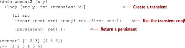
Wait, what? It seems that by using transients, you’ve made things worse—but have you? The answer lies in the question, “What am I actually measuring?” The timing code is executing zencat2 in a tight loop. This type of timing isn’t likely representative of actual use and instead highlights an important consideration: the use of persistent! and transient, although constant time in their performance characteristics, isn’t free. By measuring the use of transients in a tight loop, you introduce a confounding measure, with the disparate cost of using transients compared to the cost of concatenating two small vectors. A better benchmark is instead to measure the concatenation of larger vectors, therefore minimizing the size-relative cost of transients:
(def bv (vec (range 1e6)))

(first (time (zencat1 bv bv)))
; "Elapsed time: 181.988 msecs"
;=> 0

(first (time (zencat2 bv bv)))
; "Elapsed time: 39.353 msecs"
;=> 0
In the case of concatenating large vectors, the use of transients is ~4.5 times faster than the purely functional approach. Be careful how you use transients in your applications, because as you’ve seen, they’re an incredible boon in some cases and the opposite in others. Likewise, be careful designing performance measurements, because they may not always measure what you think.
Because transients are a mutable view of a collection, you should take care when exposing them outside of localized contexts. Fortunately, Clojure doesn’t allow a transient to be modified across threads[3] and will throw an exception if you attempt to do so. But it’s easy to forget you’re dealing with a transient and return it from a function. That’s not to say you couldn’t return a transient from a function—it can be useful to build a pipeline of functions that work in concert against a transient structure. Rather, we ask that you remain mindful when doing so.
3 On the JVM, checking for the current thread is computationally inexpensive.
Using transients can help you gain speed in many circumstances. But remember the trade-offs when using them, because they’re not cost-free operations.
15.3. Chunked sequences
With the release of Clojure 1.1, the granularity of Clojure’s laziness was changed from a one-at-a-time model to a chunk-at-a-time model. Instead of walking through a sequence one node at a time, chunked sequences provide a windowed view (Boncz 2005) of sequences some number of elements wide, as illustrated here:
(def gimme #(do (print .) %))

(take 1 (map gimme (range 32)))
You might expect this snippet to print (.0) because you’re only grabbing the first element; and if you’re running Clojure 1.0, that’s exactly what you see. But in later versions, the picture is different:
;=> (................................0)
If you count the dots, you’ll find there are 32, which is what you’d expect given the statement from the first paragraph. Expanding a bit further, if you increase the argument to range to 33, you’ll see the following:
(take 1 (map gimme (range 33)))
;=> (................................0)
Again you can count 32 dots. Moving the chunky window to the right is as simple as obtaining the 33rd element:
(take 1 (drop 32 (map gimme (range 64))))
;=> (................................................................32)
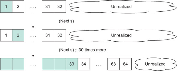
As we showed in chapter 5, Clojure’s sequences are implemented as trees fanning out at increments of 32 elements per node. Therefore, chunks of size 32 are a natural fit, allowing for the garbage collection of larger chunks of memory as shown in figure 15.1.
Figure 15.1. Clojure’s chunked sequences allow a windowed view of a sequence. This model is more efficient, in that it allows for larger swaths of memory to be reclaimed by the garbage collector and better cache locality in general. There’s a cost to total laziness, but often the benefit gained is worth the cost.
You might be worried that chunked sequences have squashed the entire point of lazy sequences, and for small sequences this is correct. But the benefits of lazy sequences are striking when dealing with cyclopean magnitudes or sequences larger than memory. Chunked sequences in extreme cases are an incredible boon because not only do they make sequence functions more efficient overall, but they also fulfill the promise of lazy sequences: avoiding full realization of interim results.
15.3.1. Regaining one-at-a-time laziness
There are legitimate concerns about this chunked model, and one such concern is the desire for a one-at-a-time model to avoid exploding computations. Assuming you have such a requirement, one counterpoint against chunked sequences is that of building an infinite sequence of Mersenne primes.[4] Implicit realization of the first 32 Mersenne primes through chunked sequences will finish long after the Sun has died.
But you can use lazy-seq to create a function seq1 that can be used to restrict (or dechunkify, if you will) a lazy sequence and enforce the one-at-a-time model:
(defn seq1 [s]
  (lazy-seq
    (when-let [[x] (seq s)]
      (cons x (seq1 (rest s))))))

(take 1 (map gimme (seq1 (range 32))))
;=> (.0)

(take 1 (drop 32 (map gimme (seq1 (range 64)))))
;=> (.................................32)
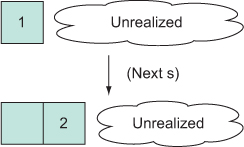
You can again safely generate a lazy, infinite sequence of Mersenne primes. The world rejoices. But seq1 eliminates the garbage-collection efficiencies of the chunked model and again regresses back to that shown in figure 15.2.
Figure 15.2. Using seq1, you can reclaim the one-at-a-time sequence model. Although not as efficient as the chunked model, it does provide total sequence laziness.
Clojure may one day provide an official API for one-at-a-time lazy sequence granularity, but for now seq1 will suffice. We advise that you instead stick to the chunked model, because you’ll probably never notice its effects during normal usage.
15.4. Memoization
As we mentioned briefly in section 10.4, memoization (Michie 1968) refers to storing a cache of values local to a function so that its arguments can be retrieved rather than calculated on every call. The cache is a simple mapping of a given set of arguments to a previously calculated result. In order for this to work, the memoized function must be referentially transparent, as we discussed in section 7.1. Clojure comes with a memoize function that can be used to build a memoized version of any referentially transparent function:
(def gcd (memoize
           (fn [x y]
             (cond
               (> x y) (recur (- x y) y)
               (< x y) (recur x (- y x))


               :else x))))
(gcd 1000645475 56130776629010010)
;=> 215
Defining a “greatest common denominator” function using memoize helps to speed subsequent calculations using the arguments 1000645475 and 56130776629010010. The function memoize wraps another function[5] in a cache lookup pass-through function and returns it. This allows you to use memoize on literally any referentially transparent function. The operation of memoize is analogous to, but not exactly the same as, the operation of Clojure’s lazy sequences that cache the results of their realized portions. This general technique can be useful, but the indiscriminate storage provided by memoize may not always be appropriate. Therefore, let’s take a step back and devise a way to generalize the operation of memoization into useful abstractions and build a framework for employing caching strategies more appropriate to the domain at hand.
5 You might have noticed that we explicitly bound the var gcd to the memoization of an anonymous function but then used recur to implement the function body. This approach suffers from the inability to cache the intermediate results (Norvig 1991) of gcd. We leave the solution to this shortcoming as an exercise for you.
Similar to Haskell’s typeclasses, Clojure’s protocols define a set of signatures that provide a framework of adherence to a given set of features. This section serves a threefold goal:
- Discussion of memoization
- Discussion of protocol design
- Discussion of abstraction-oriented programming
15.4.1. Reexamining memoization
As mentioned in section 10.4, memoization is a personal affair, requiring certain domain knowledge to perform efficiently and correctly. That’s not to say the core memoize function is useless, only that the base case doesn’t cover all cases. In this section, you’ll define a memoization protocol in terms of these primitive operations: lookup, has?, hit, and miss. Instead of providing a memoization facility that allows the removal of individual cache items, it’s a better idea to provide one that allows for dynamic cache-handling strategies.[6]
6 This section is motivated by the fantastic work of the brilliant Clojurians Meikel Brandmeyer, Christophe Grand, and Eugen Dück, summarized in Brandmeyer’s “Memoize Done Right,” http://mng.bz/0xIX.
15.4.2. A memoization protocol
The protocol for a general-purpose cache feature is provided in the following listing.
Listing 15.1. Protocol for caching
(defprotocol CacheProtocol
  (lookup  [cache e])
  (has?    [cache e] )
  (hit     [cache e])
  (miss    [cache e ret]))
The function lookup retrieves the item in the cache if it exists. The function has? checks for a cached value. The function hit is called when an item is found in the cache, and miss is called when it’s not found. Moving on, you next implement the core memoize functionality.
Listing 15.2. BasicCache type
(deftype BasicCache [cache]
  CacheProtocol
  (lookup [_ item]
    (get cache item))
  (has? [_ item]
    (contains? cache item))
  (hit [this item] this)
  (miss [_ item result]
    (BasicCache. (assoc cache item result))))
BasicCache takes a cache on construction used for its internal operations. Testing the basic caching protocol in isolation shows the following:
(def cache (BasicCache. {}))

(lookup (miss cache '(servo) :robot) '(servo))
;=> :robot
In the case of a miss, the item to be cached is added and a new instance of BasicCache (with the cached entry added) is returned for retrieval using lookup. This is a simple model for a basic caching protocol but not terribly useful in isolation. You can go further by creating an auxiliary function through, meaning in effect, “Pass an element through the cache and return its value”:
(defn through [cache f item]
  (if (has? cache item)
    (hit cache item)
    (miss cache item (delay (apply f item)))))
With through, the value corresponding to a cache item (function arguments, in this case) is either retrieved from the cache via the hit function or calculated and stored via miss. Notice that the calculation (apply f item) is wrapped in a delay call instead of performed outright or lazily through an ad hoc initialization mechanism. The use of an explicit delay in this way helps to ensure that the value is calculated only on first retrieval. With these pieces in place, you can create a PluggableMemoization type, as shown next.
Listing 15.3. Type implementing pluggable memoization
(deftype PluggableMemoization [f cache]
  CacheProtocol
  (has? [_ item] (has? cache item))
  (hit  [this item] this)
  (miss [_ item result]
    (PluggableMemoization. f (miss cache item result)))

  (lookup [_ item]
    (lookup cache item)))
The purpose of the PluggableMemoization type is to act as a delegate to an underlying implementation of a CacheProtocol occurring in the implementations for hit, miss, and lookup. Likewise, the PluggableMemoization delegation is interposed at the protocol points to ensure that when using the CacheProtocol, the Pluggable-Memoization type is used and not BasicCache. This example makes a clear distinction between a caching protocol fulfilled by BasicCache and a concretized memoization fulfilled by PluggableMemoization and through. With the creation of separate abstractions, you can use the appropriate concrete realization in its proper context.
15.4.3. Abstraction-oriented programming
Clojure programs are composed of various abstractions. In fact, the term abstraction-oriented programming is used to describe Clojure’s specific philosophy of design.
The original manipulable-memoize function from section 10.4 is modified in the following listing to conform to the memoization cache realization.
Listing 15.4. Applying pluggable memoization to a function
(defn memoization-impl [cache-impl]
  (let [cache (atom cache-impl)]
    (with-meta
      (fn [& args]
        (let [cs (swap! cache through (.f cache-impl) args)]
          @(lookup cs args)))
      {:cache cache})))
If you’ll recall from the implementation of the through function, you store delay objects in the cache, thus requiring that they be deferenced when looked up. Returning to our old friend the slowly function, you can exercise the new memoization technique as shown:
(def slowly (fn [x] (Thread/sleep 3000) x))
(def sometimes-slowly (memoization-impl
                        (PluggableMemoization.
                          slowly
                          (BasicCache. {}))))

(time [(sometimes-slowly 108) (sometimes-slowly 108)])
; "Elapsed time: 3001.611 msecs"
;=> [108 108]

(time [(sometimes-slowly 108) (sometimes-slowly 108)])
; "Elapsed time: 0.049 msecs"
;=> [108 108]
You can now fulfill your personalized memoization needs by implementing pointed realizations of CacheProtocol, plugging them into instances of PluggableMemoization, and applying them as needed via function redefinition, higher-order functions, or dynamic binding. Countless caching strategies can be used to better support your needs, each displaying different characteristics; or, if necessary, your problem may call for something new.
We’ve only scratched the surface of memoization in this section, in favor of providing a more generic substrate on which to build your own memoization strategies. Using Clojure’s abstraction-oriented programming techniques, your own programs will likewise be more generic and be built largely from reusable parts.
15.5. Understanding coercion
As a dynamic language, Clojure is designed to postpone until as late as possible decisions about how to handle specific types of values. As a practical language, Clojure allows you to specify types at compile time in some cases where doing so may significantly improve the runtime speed of your program. One way to do this is with type hints on symbols used with interop, as covered in section 15.1. Another way is through the Java primitive types that Clojure supports, which is the subject of this section.
Java primitives include variously sized numbers (byte, short, int, long, float, and double) as well as boolean and char types. Each of these has a counterpart that is a normal class spelled with a capital first letter: for example, an int value can be boxed up and stored in an instance of Int. Java primitives can improve performance a lot because they use less memory, generate less memory garbage, and require fewer memory dereferences than their boxed counterparts. These primitives are useful both with interop and with Clojure functions that have been defined specifically to support primitives, although Clojure functions only support primitive arguments of type long and double.
To see the value of primitives, consider this factorial function, which is a favorite of micro-benchmarkers everywhere.
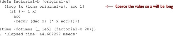
Listing 15.5. Tail-recursive factorial, with no type declarations
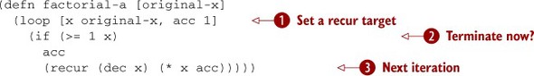
This may not be the most natural way to define factorial, because instead of using nesting recursion, it uses the recur operator in the tail position (see section 2.6.3). You do this so the recursion consumes no stack. Try it, and observe how quickly the result of factorial grows very large:
(factorial-a 10)
;=> 3628800

(factorial-a 20)
;=> 2432902008176640000
This chapter is about performance, so you should measure the function’s speed. Be sure to run this a few times to give the JVM a chance to optimize it:
(time (dotimes [_ 1e5] (factorial-a 20)))
; "Elapsed time: 172.914384 msecs"
This is the baseline: 100,000 calls of (factorial 20) in under 200 milliseconds. To see how coercion can help, you need to think about what the Clojure compiler knows about the type of each expression.
15.5.1. Using primitive longs
Starting with Clojure 1.3, literal numbers compile as primitives. Look back at listing 15.5 to see the primitive literals at ![]() and
and ![]() . This means Clojure knows that acc is a long, so the use of dec at
. This means Clojure knows that acc is a long, so the use of dec at ![]() should be taking advantage of that. But the type of x is unknown to the compiler, which means the comparison and the multiplication must be compiled in a way that it will work
regardless of the actual numeric type encountered at runtime. If you want x to be a primitive long, you can coerce it where it’s defined in loop as shown in the next listing. This kind of coercion also works in let forms.
should be taking advantage of that. But the type of x is unknown to the compiler, which means the comparison and the multiplication must be compiled in a way that it will work
regardless of the actual numeric type encountered at runtime. If you want x to be a primitive long, you can coerce it where it’s defined in loop as shown in the next listing. This kind of coercion also works in let forms.
Listing 15.6. Factorial with a coerced local
Another way to get similar results is to declare the type of the function parameter, as shown in listing 15.7. This looks like type hinting but isn’t. Whereas type hints can only refer to class names and only influence the compilation of interop forms, functions with primitive arguments are compiled to code that coerces inputs to the declared types so that interop and math functions can assume the primitive type.
Listing 15.7. Factorial with a primitive long argument
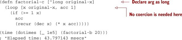
By avoiding the boxing and unboxing of x in both these listings, you have a function that runs around four times faster for this test. But you can avoid even more work. Specifically, every time a number is computed, it’s checked to make sure it falls within the range of the type it’s using (in this case, long). And longs are huge, so surely you don’t need to worry about out-of-range values. The following listing shows how to turn off the overflow checking.
Listing 15.8. Factorial without overflow checking

Timing this shows impressive results:
(time (dotimes [_ 1e5] (factorial-d 20)))
; "Elapsed time: 15.674197 msecs"
This is another doubling or more of the function’s speed. Unfortunately, you’ve introduced an error that can be extremely difficult to find:
(factorial-d 21)
;=> -4249290049419214848
A factorial should never produce a negative number, and yet there it is. By turning off overflow checking, you can generate incorrect results without even noticing, and you have no easy way to find the source of the problem. This is in stark contrast to the default behavior, which you can observe by trying the original factorial-a version:
(factorial-a 21)
; ArithmeticException integer overflow
The stack trace generated by this exception shows not only the use of multiplication that sent the accumulator outside the range of long, but also the entire call chain that led to it. This is much more helpful than a silently incorrect result. You might consider using unchecked math, but only very carefully—perhaps by manually including checks at larger-grained places for inputs that will cause out-of-bounds results. Most of the time, it’s best to leave overflow checking on and accept the performance hit, which in most real-world situations isn’t as dramatic as shown in this example.
Although the primitive long type turned out to be a poor choice for factorial, in many situations a long is perfectly acceptable. In these cases, using primitive longs with overflow checking on may be an ideal compromise between safety and performance.
But what if you have an application somewhat like factorial, and you want neither an incorrect answer nor an overflow exception for small input values like 21? We’ll explore two different solutions, each with its trade-offs. The first sacrifices only accuracy, and the second sacrifices only performance.
15.5.2. Using primitive doubles
One way to avoid overflow is to use a floating-point representation. Because Clojure has broad support for primitive doubles, it’s reasonable to try replacing long with double in your function definition. Let’s try this in the next listing, updating the literals to be doubles as well for better performance.
Listing 15.9. Factorial with a primitive double argument
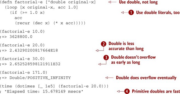
As promised, doubles give up accuracy, as shown at ![]() and
and ![]() ; but they deliver excellent performance, as shown at
; but they deliver excellent performance, as shown at ![]() . Note that the literals at
. Note that the literals at ![]() and the previous line are written as 1.0 instead of 1 so they will be compiled as literal doubles instead of longs. Using longs would have meant mixed types for the multiplication,
which would hurt performance (but only slightly).
and the previous line are written as 1.0 instead of 1 so they will be compiled as literal doubles instead of longs. Using longs would have meant mixed types for the multiplication,
which would hurt performance (but only slightly).
Again, this seems to be a poor choice for factorial, but there are domains where the inaccuracy of floating-points isn’t a problem and their range is sufficient for the domain. In these domains, the performance provided by primitive doubles can be fantastic.
Let’s examine one more solution, giving up some performance in order to maintain perfect accuracy.
15.5.3. Using auto-promotion
Prior to Clojure 1.3, math operations auto-promoted to number objects that could handle arbitrary precision when necessary. Although this behavior is no longer the default, sometimes it’s exactly what you want, and so it’s provided in the prime math operators: +', -', *', inc', and dec'. These are spelled just like their non-promoting counterparts, but with trailing single-quote character. The following listing uses *' to allow acc to be promoted but continues to use a primitive long for x on the assumption that nobody wants to wait for this factorial function to iterate Long/MAX_VALUE times.
Listing 15.10. Factorial with auto-promotion

Using a primitive long for original-x as declared at ![]() allows Clojure to assume x is also a primitive long. Together this gives performance that beats the baseline back in listing 15.5.
allows Clojure to assume x is also a primitive long. Together this gives performance that beats the baseline back in listing 15.5.
The use of auto-promoting multiplication at ![]() produces an arbitrary-precision BigInt object when needed, which is visible in the trailing N in the result of
produces an arbitrary-precision BigInt object when needed, which is visible in the trailing N in the result of ![]() . Clojure uses its own BigInt for arbitrary-precision integers like this and Java’s Big-Decimal for arbitrary-precision decimal reals. Literals for BigDecimal can be written with a trailing M, but don’t forget about the option of using rationals when dealing with non-integers (see section 2.7.2).
. Clojure uses its own BigInt for arbitrary-precision integers like this and Java’s Big-Decimal for arbitrary-precision decimal reals. Literals for BigDecimal can be written with a trailing M, but don’t forget about the option of using rationals when dealing with non-integers (see section 2.7.2).
This finally seems like a good compromise for the implementation of factorial, but let’s review the coercion options we considered. We showed that numbers can be represented as either primitive or boxed. Primitives are prone to overflow but provide the best performance and can even be used in dangerous unchecked ways. Boxed numbers are slower but can be used with auto-promoting math operations to maintain arbitrary precision. And, of course, you can choose the most appropriate type for each local to achieve the desired trade-off between behavior and performance.
15.6. Reducibles
Modern languages often provide a common interface for all their collection types, such as some kind of iterator interface. In Clojure, this is naturally supplied by the seq abstraction. Much of the power of these interfaces derives from their minimalism—their requirements are so humble that it’s easy for a new collection type to comply. This leads to a ubiquity that allows users of the abstraction to work across a powerfully wide range of collections.
Clojure’s seq abstraction is indeed minimal, requiring the implementation of essentially just first and rest. But Clojure 1.5 provides even more minimal [7] collection interfaces, CollReduce and CollFold, each of which requires a single method to be implemented. We’ll come to the justification for these interfaces later, but for now try to be satisfied with the proposition that a more minimal interface may be more powerful and possibly lead to better performance.
7 You’ll see later why the good ol’ seq abstraction continues to be useful as well.
15.6.1. An example reducible collection
In some programming languages (Ruby springs to mind), a range is an object that denotes a start value, an end value, and the steps in between. Although Clojure has a range function that builds a sequence of numbers based on these criteria, a range isn’t a first-class object in Clojure. But you can think of a range as a collection that is traversed and built according to the dictates of the start, end, and step values. The following listing implements a version of range that requires these three elements and returns a lazy sequence of numbers. It follows the lazy-seq recipe set out earlier by starting with the lazy-seq macro, then checking for the termination case, and finally constructing a cons cell of the current and remaining values.
Listing 15.11. Reimplementing Clojure’s range function using lazy-seq

Although interesting (maybe), the lazy sequence returned from lazy-range is nothing special, but it probably behaves as you expect:
(lazy-range 5 10 2)
;=> (5 7 9)

(lazy-range 6 0 -1)
;=> (6 5 4 3 2 1)
Given the lazy sequences returned here, it’s easy to produce another collection such as a vector, or compute some other reduced value such as a sum:
(reduce conj [] (lazy-range 6 0 -1))
;=> [6 5 4 3 2 1]

(reduce + 0 (lazy-range 6 0 -1))
;=> 21
Both of these are perfectly reasonable things to do with a lazy sequence, but neither takes advantage of the signature feature of a lazy sequence: laziness. Even though they don’t need laziness, they’re still paying for it by allocating a couple objects on the heap for each element of the range. So instead of returning a lazy seq, what if you were to return a function that acted like reduce? Let’s call this function a reducible:
(fn [reducing-fn initial-value]
  ;; ...

  ;; returns the reduced value
)
Rather than pass the reducible to reduce as you did with the lazy seq, in order to execute the reduction and produce the final reduced value, you call the reducible. If you had a version of lazy-range that built collections following the minimal collection interface named reducible-range, you could use it as follows:
(def countdown-reducable (reducible-range 6 0 -1))

(countdown-reducible conj [])
;=> [6 5 4 3 2 1]

(countdown-reducible + 0)
;=> 21
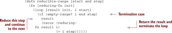
This is the more minimal collection interface—a function that can be used to extract the contents of the collection, as you did with conj and [], or to produce some other derived value. The definition of reducible-range demonstrated here is given in the following listing. This is different from lazy-range primarily in that it drives the reduction loop itself, using loop and recur, and finally returns the reduced value instead of terminating with nil.
Listing 15.12. Reimplementation of range that returns a reducible
15.6.2. Deriving your first reducing function transformer
You may be wondering how this reducible, a mere function, can possibly support anything like the wide range of manipulations that lazy seqs support. How can a reducible be filtered or mapped when all you can do with it is call it? This is a troubling question, and to help answer it we’ll take a step back and look at what exactly it means to map a sequence. Then we’ll examine how well the answer extends to filtering and concatenating.
Let’s begin with an easy-to-grasp function that you’d like to map across a collection. That function is half:
(defn half [x]
  (/ x 2))

(half 4)
;=> 2

(half 7)
;=> 7/2
In the context of using reduce, the easiest way to use half is to combine it with a reducing function like + to make a new reducing function. Let’s call this one sum-half, because it sums up the halves of the inputs:
(defn sum-half [result input]
  (+ result (half input)))

(reduce sum-half 0 (lazy-range 0 10 2))
;=> 10

((reducible-range 0 10 2) sum-half 0)
;=> 10
You can map across the input values, halving them as you go, but so far only by hard-coding the mapping function half and the reducing function + into a new function. This is the essence of mapping only as much as Paul McGann’s Doctor is the essence of The Doctor[8] or margarine is the essence of butter. To get where you want to be, you need to change these hard-coded functions into parameters. Begin by wrapping sum-half in another function that takes the + function (or any other reducing function) as a parameter:
8 An argument can be made for Tom Baker, but we digress.
(defn half-transformer [f1]
  (fn f1-half [result input]
    (f1 result (half input))))
First notice how f1-half is nearly identical to sum-half. Then notice how many of the functions here are reducing functions in that they take two arguments, a previous result or seed and an input, and return a new result: sum-half and f1-half are reducing functions, as are f1 and +. This is why you can describe the previous function as a transformer, specifically a reducing function transformer, because it takes one reducing function (f1) and returns another (f1-half).
You can of course use this directly, just as you did sum-half:
((reducible-range 0 10 2) (half-transformer +) 0)
;=> 10

((reducible-range 0 10 2) (half-transformer conj) [])
;=> [0 1 2 3 4]
But you’re not done yet, because half is still hard-coded. So you repeat the same pattern as last time by wrapping half-transformer in another function that takes half (or any other mapping function) as a parameter, and derive mapping as shown next.
Listing 15.13. Essence of mapping, bundled to be used with a reducible

Compare mapping with half-transformer, and note that you again replace a specific function with a parameter. But this time, neither the parameter map-fn nor what it returns (map-transformer) is a reducing function. They’re two different sorts altogether. map-fn takes a single input and returns a single result (making it a mapping function), whereas map-transformer, as we said, is a transformer. So mapping isn’t any kind of transformer; it’s a transformer constructor. Functions of this variety take whatever parameters they need but always return reducing function transformers. Feel free to consult table 15.1 if you’re starting to feel flustered by all the different kinds of functions.
Table 15.1. The various kinds of reducer-related functions
|
Name |
Parameters |
Return value |
Example |
|---|---|---|---|
| Mapping function | Input | Mapped output | half |
| Reducing function | Previous result, next input | Reduced value | sum-half |
| Reducible | Reducing function, init value | Reduced value | (reducible-range 0 5 1) |
| Reducible constructor | Various | Reducible | reducible-range |
| Reducing function transformer | Reducing function | Reducing function | half-transformer |
| Transformer constructor | Various | Reducing transformer | mapping |
You now have a function in which everything has been abstracted away except the core idea of what it means to map a value, and that idea is bundled into a form that can be applied to reducibles. With these two abstractions, reducibles and mapping, you can do quite a bit:
((reducible-range 0 10 2) ((mapping half) +) 0)
;=> 10

((reducible-range 0 10 2) ((mapping half) conj) [])
;=> [0 1 2 3 4]

((reducible-range 0 10 2) ((mapping list) conj) [])
;=> [(0) (2) (4) (6) (8)]
The syntax falls short of what you might hope for, and it certainly doesn’t look like a drop-in replacement for lazy seqs yet. We’ll see what we can do about the syntax a little later. For now, we should explore more deeply the power available with reducibles and also what we’re giving up compared to lazy seqs.
15.6.3. More reducing function transformers
Mapping allows a broad range of transformations to collections, as long as the output collection is the same size as the input. One way to produce a smaller collection is with filter, which can be implemented as shown in the following listing.
Listing 15.14. Essence of filtering, bundled to be used with a reducible

There are exactly three important differences between the filtering and mapping functions:
- Unsurprisingly, filtering has an if where mapping had none. The given predicate is tested against the input and either included
 or ignored
  .
.
- The reducing call to f1[9] is almost identical, except the input is passed through untouched instead of being passed through a mapping function. We
could certainly imagine a different form of the filtering function that supported a mapping function as well, but we’ll show in a moment why that’s unnecessary.
9 Clojure’s implementation of reducers in clojure.core.reducers frequently uses the name "f1"" for a reducing function passed in to a transformer.
- When the predicate returns false, this iteration of the filter must have no impact on the accumulating result, so the result passed in is returned unchanged.
Using filtering with a reducible is just like using mapping:
((reducible-range 0 10 2) ((filtering #(not= % 2)) +) 0)
;=> 18

((reducible-range 0 10 2) ((filtering #(not= % 2)) conj) [])
;=> [0 4 6 8]
If you wish to map the values with a mapping function either before or after filtering, you can do so by combining calls to mapping and filtering. Remember that conj and + in the previous example are reducing functions, which is the same kind of function that transformers take and return. And because (mapping half) and (filtering #(not= % 2)) are both transformers, they can be chained together like so:
((reducible-range 0 10 2)
  ((filtering #(not= % 2))
    ((mapping half) conj))
  [])

;=> [0 2 3 4]
That is, the reducible calls the function returned by filtering for each value of the sequence. The filtering function calls the function returned by mapping only for those values that pass the predicate supplied as filtering’s argument. It’s left up to the mapping function to use conj to add only those values to the resulting sequence.
In the previous code, you replaced conj with ((mapping half) conj), so after filtering the values they were divided in half before being conjed onto the resulting vector. Because the use of filtering left out the number 2, it’s the number 1 that is missing from the final vector. You can map before filtering, if you’d rather, by nesting them in reverse:
((reducible-range 0 10 2)
  ((mapping half)
   ((filtering #(not= % 2)) conj))
  [])

;=> [0 1 3 4]
Here you do the mapping first: only after 4 has been divided by 2 does filtering exclude the resulting 2 from the final vector.
Now that you’ve seen reducibles adjusted in ways that remove some elements (filtering) and leave the number of elements alone (mapping), look at the next listing to see how to construct a transformer that adds elements in the same way mapcat does for lazy seqs.
Listing 15.15. Essence of mapcatting, bundled to be used with a reducible

The interesting difference here is that mapcatting expects map-fn to return a reducible, which then must be merged into the result. So the returned reducible is called with the previous result as its starting point, passing f1 on through.
To demonstrate this, you need a little helper function for map-fn that takes a number from reducible-range and returns a new reducible:
(defn and-plus-ten [x]
  (reducible-range x (+ 11 x) 10))

((and-plus-ten 5) conj [])
;=> [5 15]
Now you can pass that to mapcatting and see how the resulting reducibles are all concatenated:
((reducible-range 0 10 2) ((mapcatting and-plus-ten) conj) [])
;=> [0 10 2 12 4 14 6 16 8 18]
We’ve shown a nice range of composable functionality on top of reducibles, but the syntax leaves quite a bit to be desired. Fortunately, this can be fixed.
15.6.4. Reducible transformers
One key difference between the way sequence functions are composed and what you’ve been doing with reducibles is that the examples have been piling on to the reducing function instead of the collection. That is, you’re used to modifying the collection and getting a new collection that can be reduced later:
(filter #(not= % 2)
  (map half
       (lazy-range 0 10 2)))
;=> (0 1 3 4)
In order to compose reducing function transformers in a similar way, you need to turn them into reducible transformers instead. The new reducible transformers must take as parameters not just the reducing function that the transformer constructors took, but also a reducible that acts as input. These two parameters correspond to the half and lazy-range that map is given in the previous snippet. Here’s how these reducible transformers are written for map and filter.
Listing 15.16. A couple of reducible transformers
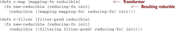
Both these functions take the two parameters we just described and return a new reducible. Remember, a reducible is just a function that takes a reducing function and a starting value, and returns the result of running that reducing function across the entire collection. In this case, the collection is described by the passed-in reducible. But between that and the init, you interject your own reducing function, wrapping the user’s reducing-fn by passing it to the reducing function transformer created by calling either mapping or filtering.
With r-map and r-filter defined, you can now write reducible pipelines of the same shape as the equivalent lazy sequence pipeline:
(def our-final-reducible
  (r-filter #(not= % 2)
            (r-map half
                   (reducible-range 0 10 2))))

(our-final-reducible conj [])
;=> [0 1 3 4]
The similarities between the implementations of r-map and r-filter are obvious and suggest the repeated code could be factored out. Clojure’s clojure.core.reducers namespace does exactly this, using the function reducer, which we’ll look at in a moment.
15.6.5. Performance of reducibles
Having achieved a code shape nearly identical to that of a lazy sequence, you might be wondering what the benefit is of this new collection abstraction. Although you’ll see some side benefits later, the primary win is performance. You can use criterium, a third-party Clojure library (https://github.com/hugoduncan/criterium),[10] to measure the performance of Clojure expressions. We measured a reduction across a two-step pipeline on our own lazy-range:
10 Our project.clj file includes :dependencies [[criterium "0.3.0"]].
(require '[criterium.core :as crit])
(crit/bench
  (reduce + 0 (filter even? (map half (lazy-range 0
             (* 10 1000 1000) 2)))))
; Execution time mean : 1.593855 sec
That is 10 million numbers mapped, filtered, and added in just over 1.5 seconds, which gives us a baseline to improve on. Since version 1.1, Clojure itself has improved on this with chunked sequences, which we discussed in section 15.3. Clojure’s lazy range function returns a chunked sequence that can be reduced more efficiently than lazy-range:
(crit/bench
 (reduce + 0 (filter even? (map half (range 0 (* 10 1000 1000) 2)))))
; Execution time mean : 603.006967 ms
This helps a lot. By allocating and processing chunks of the lazy sequence at a time, instead of individual cons cells, the work gets done more than 60% faster. How do reducibles fare?
(crit/bench
 ((r-filter even? (r-map half
     (reducible-range 0 (* 10 1000 1000) 2))) + 0))
; Execution time mean : 385.042958 ms
In this case, we get another 35% improvement beyond what chunked seqs provided. But again, a critical difference is that this difference was achieved via a simpler interface and naive implementations rather than the more complex interface and implementations demanded by chunked sequences. Reducers seem to be a win.
The range of expressions that can be built out of this reducible abstraction is remarkable. Many of the composable processing functions you’re familiar with from lazy seqs can be brought over, and all this with nothing but closures and function calls—not a cons cell or deftype in sight. But there are a few trade-offs, as you might expect.
15.6.6. Drawbacks of reducibles
The primary drawback of reducibles is that you give up laziness. Because the reducible collection is responsible for reducing its entire contents, there’s no way, short of shenanigans with threads or continuations, to suspend its operation in the way we regularly do with lazy seqs. This gets in the way of reducibles efficiently consuming multiple collections at once, the way map and interleave do for lazy seqs.
The closest Clojure’s implementation comes to supporting suspension is early termination. You can use reduced to mark that a reduction loop should be terminated early, and reduced? to test for this case.
15.6.7. Integrating reducibles with Clojure reduce
So far you’ve worked with reducibles that are functions. This is fine as long as reducing is the only thing you need to do with them. But real collections have to support being built up such as with conj or assoc and may want to support other interfaces such as Seqable for getting lazy seqs or ILookup for random access. In short, they must implement many interfaces, not just the most minimal and ubiquitous interface.
This is why Clojure provides the clojure.core.protocols.CollReduce protocol instead of using function-based reducibles as we introduced earlier. To make the previous work integrate with Clojure’s reducers framework, we need to address this protocol. As is usual with protocols, two sides must be addressed: the implementation of the protocol (making reducible-range available by calling coll-reduce) and the use of the protocol (making mapping and friends call coll-reduce). From now on, when we refer to core reducibles, transformers, and so on, we mean those made to work with Clojure’s CollReduce and related protocols, in contrast to the function-based ones we discussed in previous sections.
Let’s begin by making reducing function transformers work with Clojure collections. Clojure makes this easy with the reducer function, which automates the kind of transformation you did to define r-map and r-filter back in listing 15.16. But reducer returns a core reducible (that is, an object that implements CollReduce), so you can use it to define a couple new functions as in this listing.
Listing 15.17. Converting transformers to core reducibles

Now you can use the functions like this:
(reduce conj []
        (core-r-filter #(not= % 2)
                       (core-r-map half [0 2 4 6 8])))
;=> [0 1 3 4]
You use a vector as input to the pipeline because vectors already implement Coll-Reduce, which makes them core reducibles themselves. The new transformers, core-r-map and core-r-filter, also return core reducibles. Finally, the reduce function in Clojure 1.5 knows how to work not only with sequences but also with core reducibles, so the entire pipeline is executed the same way as the function-based reducibles were earlier.
If you want to provide your own reducible-range as a core reducible, the second side of the protocol implementation, you have to do a bit more work. Specifically, you need to implement it via a protocol instead of a function.
Listing 15.18. Implementing a reducible-range via the CollReduce protocol
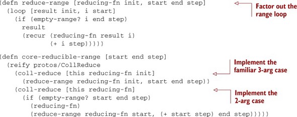
You need to run the main range-reducing loop from a couple different contexts, so here you abstract it out and have it take all five parameters (separating the reduce args from the range args with a comma). This is nearly identical to the definition of reducible-range back in listing 15.12, but it’s defined here with no closure and thus less memory allocation when run.
Now that reduce-range is factored out, implementing the three-argument form of coll-reduce is easy. The two-argument form of coll-reduce corresponds to the two-argument form of reduce. That is, the first item of the collection is used as the seed or init value of the reduction. You do this by peeling off the start value and calling reduce-range with that as the init and shorter-by-one remainder of the range.
This form also means you must deal with the possibility of an empty collection with no init value to return. In this case, Clojure’s definition of reduce requires you to return the result of calling the reducing function with no arguments.
Together, this allows you to use core-reducible-range with Clojure’s reduce function in all the normal ways:
(reduce conj []
        (core-r-filter #(not= % 2)
                       (core-r-map half
                                   (core-reducible-range 0 10 2))))
;=> [0 1 3 4]


(reduce + (core-reducible-range 10 12 1))
;=> 21

(reduce + (core-reducible-range 10 11 1))
;=> 10

(reduce + (core-reducible-range 10 10 1))
;=> 0
You’ve now seen the simplicity of the reducibles interface and how it can improve performance while providing syntax nearly identical to Clojure’s seq library. By using protocols, you can even use some of the same functions and collections you already know, like reduce and vectors. But it’s possible to get results even faster by giving up more guarantees. If you don’t care about the order in which your reducing functions are called, several of them can be run in parallel.
15.6.8. The fold function: reducing in parallel
We briefly mentioned fold back in chapter 11, but now we have covered enough background to look more closely at how it works. All the reduce and reduce-like operations we’ve discussed so far have worked in a linear fashion, starting at the beginning of a collection and proceeding in order. But as we pointed out in chapter 11, in many situations the reducer we want to use is associative and doesn’t need to proceed in order. So just as with lazy seqs versus reducibles, our abstraction is too specific, promises too much, and as a consequence isn’t useful in some situations where it could be.
The alternative to reduce that supports parallel instead of sequential operation is called fold. The clojure.core.reducers/fold function is similar to reduce. In its shortest form, it can take exactly the same parameters as reduce and return the same result:
(reduce + [1 2 3 4 5])
;=> 15

(r/fold + [1 2 3 4 5])
;=> 15
The primary difference is that it doesn’t make any promises about order of execution and requires that your reducing function be associative.[11] This gives fold the freedom it needs to do the divide-and-conquer work for you.
11 Actually, if your reducing function is different than your combining function, only the combining function must be associative. We’ll get to combining functions soon.
This ties in to the reducibles abstraction, because all the reducing function transformers we’ve presented (mapping, filtering, and mapcatting), as well as many others, if given a pure associative reducing function, will return another pure associative reducing function. In other words, they’re as compatible with the requirements of fold as they are with reduce, and as a result they can be made similarly available with a conversion function provided in the reducers namespace.
Listing 15.19. Converting transformers to core foldables

These new foldable transformers can now be used with fold:
(r/fold +
        (core-f-filter #(not= % 2)
                       (core-f-map half
                                   [0 2 4 6 8])))
;=> 8
Alas, they’re unnecessary, because Clojure’s reducers library provides them already, under the names map and filter:
(r/fold +
        (r/filter #(not= % 2)
                  (r/map half
                         [0 2 4 6 8])))
;=> 8
Also provided are a few other functions whose names and behavior will be familiar to anyone who knows the seq library. These currently include drop, filter, flatten, map, mapcat, remove, take, and take-while.
So far we’ve only looked at the two-argument form of fold. Like reduce, fold has more complex forms, but they’re different than reduce’s. One of the optional parameters that fold takes is a combining function. We’ll look at that in more detail in a moment, but for now keep in mind that if you don’t specify one, fold will use your reducing function for combining as well.
Another difference is that fold doesn’t take an initial or seed value as a parameter. Instead, it calls the combining function with no arguments to determine an initial value. For example, if you wanted to sum up some values but start with an initial value of 100, you could do it like this:
(r/fold (fn ([] 100) ([a b] (+ a b))) (range 10))
;=> 145
Here you supply a reducing function that takes either no parameters, in which case it returns 100, or two parameters a and b and returns their sum. You didn’t need this in the earlier example of fold because the + function returns zero when called with no arguments, which is often exactly what you want.
But when you do want to provide an initial value, the two-body function syntax just demonstrated is a bit awkward, so Clojure provides a tool to build such functions for you. This tool is a function called monoid that takes an operator (+ in this example) and a constructor that returns the initial value. You could write the previous example like this:
(r/fold (r/monoid + (constantly 100)) (range 10))
;=> 145
Now on to the combining function. As mentioned previously, fold divides the work to be done into smaller pieces and reduces all the elements in each piece. By default, each piece has approximately 512 elements, but this number can be specified as an optional parameter to fold. When two pieces of work have been done and need to be combined, this is done by calling the combining function, another optional parameter to fold. With all default arguments given, the previous example is equivalent to

If you don’t specify a combining function, the reducing function will be used. This makes sense when the reducing function accepts two parameters of the same type it returns, such as when using + for summing up the numbers in a collection as we showed previously. But for some operations this isn’t the case, such as when conjing elements into a vector. In this case, when fold is reducing the small pieces of work, it’s conjing individual elements into a vector. But when combining these pieces of work, it has two vectors—combining this with conj won’t achieve the desired results:
(r/fold 4 (r/monoid conj (constantly [])) conj (vec (range 10)))
;=> [0 1 [2 3 4] [5 6 [7 8 9]]]
Using conj on two vectors puts the second inside the first, instead of joining them into a single vector, which is what produces the mess of nested vectors shown here.
The combining function we’re looking for is into, which, when given two vectors, joins them into a single vector in the natural order, like this:
(r/fold 4 (r/monoid into (constantly [])) conj (vec (range 10)))
;=> [0 1 2 3 4 5 6 7 8 9]
It’s interesting to consider how the reducing and combining steps together give us the tools we need to solve the same kinds of problems that map/reduce frameworks do, and with fold we can run them in a similarly parallel way. And just as with map/reduce jobs, we often need to provide custom functions for the reducing and combining steps, as well as transformers for the input collection. But our specific example of combining all the elements from a foldable into a collection is common enough that Clojure provides a high-performance function to do exactly that: foldcat. It doesn’t build a vector, but it does internally call fold using reducing and combining functions that efficiently build a collection that is reducible, foldable, sequable, and counted. You can use it like this:
(r/foldcat (r/filter even? (vec (range 1000))))
;=> #<Cat clojure.core.reducers.Cat@209bc0df>

>(seq (r/foldcat (r/filter even? (vec (range 10)))))
;=> (0 2 4 6 8)
What has all this splitting up of work and recombining bought us in terms of performance? If you recall, the fastest our benchmark ran using reducers was 385 milliseconds. Let’s see what fold can do:
(def big-vector (vec (range 0 (* 10 1000 1000) 2)))

(crit/bench
 (r/fold + (core-f-filter even? (core-f-map half big-vector))))
;; Execution time mean : 126.756586 ms
We used a vector here because none of the range functions currently available return a foldable collection. But even accounting for that difference, fold still gets the job done at least 55% faster on our test machine. Of course, many factors may cause you to see different results, not the least of these being the number of processor cores used for the test; but nevertheless it’s clearly a marked improvement.
In this section, you’ve seen how a minimal abstraction can be built up from simple functions and used as a basis for higher-performance collection processing. You’ve also seen how that can be combined with weaker promises about order of operation to provide parallelism and even higher performance.
15.7. Summary
Clojure provides numerous ways to gain speed in your applications. Using some combination of type hints, transients, chunked sequences, memoization, and coercion, you should be able to achieve noticeable performance gains. Like any powerful tool, these performance techniques should be used cautiously and thoughtfully. But once you’ve determined that performance can be gained, the use of these techniques is minimally intrusive and often natural to the unadorned implementation.
In the next chapter, we’ll cover a topic that has captured the imagination of a growing number of Clojure programmers: logic. Clojure is an excellent programming language for exploring new ways of thinking, and although logic programming isn’t new, it leads to different ways of thinking about solving problems.