Chapter 16. Thinking programs

Search in book...
Toggle Font Controls
Create new playlist

Name your new playlist

Playlist description (optional)
Sign In

Email address

Password

Forgot Password?

or

Continue with Facebook

Continue with Google
Sign Up

Full Name

Email address

Confirm Email Address

Password

or

Continue with Facebook

Continue with Google

Chapter 16. Thinking programs

This chapter covers

Searching
Thinking data via unification
Logic programming
Constraint programming

Functional programming is an attempt to reach a declarative ideal in program composition. Functional techniques can lead to code that mirrors the form of the solution, but sometimes levels of expressiveness come at a cost in terms of speed. In problems of search, for example, matters related to the “how” of search intermingle with the “what” of the solution. In this chapter, we’ll explore matters of search and querying using functional approaches compared to logical techniques.

We’ll start by discussing search and building a Sudoku solver that uses a brute-force functional approach that strives to solve the problem declaratively. Next we’ll explore the idea of thinking data using a special kind of pattern matching called unification. Our exploration of unification will transition into a discussion of a promising Clojure contrib library called core.logic. The core.logic library provides a logic-programming system allowing declarative descriptions of problem spaces that actually run. We’ll conclude this chapter by exploring ways to constrain the search space involved in solving logic problems to speed up execution times.

16.1. A problem of search

Logic programming is largely a matter of search. To solve a problem requiring logic requires you to explore the sea of possibilities available. Many logic programming languages (such as Prolog) are abstractions over the act of searching trees of possible solutions to a query. This isn’t a book about Prolog, but often you’ll find yourself needing to search a vast space to solve a tricky problem. For example, Prolog is often used to implement systems containing many business rules that can interact and counteract in a huge number of ways.

When we think of searching, the subject of games and puzzles often comes to mind. Game and puzzle searches provide a nice Petri-dish environment for exploring logic programming and search-space culling. In this section, we’ll talk about a simple type of puzzle called Sudoku and explore an inefficient approach to searching for solutions to puzzles.

16.1.1. A brute-force Sudoku solver

The game Sudoku is a vaguely mathematical puzzle with a few advantages for the purpose of exploration. First, the rules of Sudoku are simple to describe and are therefore easy to encode in code. Second, a naive Sudoku solver can be created in a few lines of code. We’ll show you how to create such a solver for the purpose of introducing some logic programming concepts.

Here’s a description of what a Sudoku game looks like:

You start with a 9 × 9 square.
The square is subdivided into nine 3 × 3 sections.
Some of the spaces in the square contain numbers.

The objective is to fill the empty spaces so that the following puzzle constraints are satisfied:

Each column must contain one occurrence of each digit from 1–9.
Each row must contain one occurrence of each digit from 1–9.
Each 3 × 3 subsection must contain one occurrence of each digit from 1–9.

Figure 16.1 shows the Sudoku board you’ll use for the example in this chapter.

Figure 16.1. Starting position of the example Sudoku board

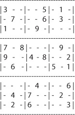
You can create a bare-bones representation of this board using a Clojure vector like the following:

(def b1 '[3 - - - - 5 - 1 -
          - 7 - - - 6 - 3 -
          1 - - - 9 - - - -
          7 - 8 - - - - 9 -
          9 - - 4 - 8 - - 2
          - 6 - - - - 5 - 1
          - - - - 4 - - - 6
          - 4 - 7 - - - 2 -
          - 2 - 6 - - - - 3])

Although it’s convenient for entry, this board doesn’t look anything like a Sudoku board, so let’s define a function prep that makes it more accurate:

(defn prep [board]
  (map #(partition 3 %)
       (partition 9 board)))

This function does what you might expect: it segments the board into the divisions expected for a 9 × 9 Sudoku board. Now you can write a simple, imperative board printer to print the textual board shown in figure 16.1; the function print-board is given next.

Listing 16.1. Printing the starting position of a Sudoku board

(defn print-board [board]
  (let [row-sep (apply str (repeat 37 "-"))]
    (println row-sep)
    (dotimes [row (count board)]
      (print "| ")
      (doseq [subrow (nth board row)]
        (doseq [cell (butlast subrow)]
          (print (str cell "   ")))
        (print (str (last subrow) " | ")))
      (println)
      (when (zero? (mod (inc row) 3))
        (println row-sep)))))

As is often the case when printing, the structure of print-board is highly declarative. All you’re doing is looping through each row and printing each entry, with a special character to denote subgrid sections. The function print-board is used as follows:

(-> b1 prep print-board)

Now that the technicalities are out of the way, we can move on to the mechanics of implementing a solver.

The regions of a Sudoku board

As we explained earlier, the objective of Sudoku is to complete the square such that each column, each row, and each 3 × 3 subsection contains one occurrence of every digit from 1–9. As it turns out, making the board into a more reasonable representation works well for printing, but it’s nicer to keep it flat for calculating groupings. This means for any cell on the board, you’ll calculate three things:

The row containing the cell
The column containing the cell
The 3 × 3 subgrid containing the cell

To get these pieces of information, you’ll write three auxiliary functions: row-for, column-for, and subgrid-for. The implementation of row-for is as follows:

(defn rows [board sz]
  (partition sz board))

(defn row-for [board index sz]
  (nth (rows board sz) (/ index 9)))

This is similar to the implementation of the rank-component shown way back in listing 1.6. Its entire purpose is to take a one-dimensional coordinate in a vector and map it onto the logical two-dimensional space of the Sudoku board. It does this by using the helper function rows to slice the board into rows and taking the one containing the adjusted (by 9) index. Testing the implementation for the first empty cell at index 1 gives the following result:

(row-for b1 1 9)
;=> (3 - - - - 5 - 1 -)

This matches the first row for board b1. Moving on, the column-for implementation is somewhat similar:

(defn column-for [board index sz]
  (let [col (mod index sz)]
    (map #(nth % col)
         (rows board sz))))

The difference is that you don’t preprocess the board into columns, but instead grab the precise column you need. You can do this because you provide a specific size for the columns and go to the correct place with some mod math. Testing the function quickly for the column at index 2 gives this result:

(column-for b1 2 9)
;=> (- - - 8 - - - - -)

The explicit-size approach is useful. You need the same behavior when you grab the columns of the subgrids using subgrid-for:

The subgrid-for function is unfortunately a complex beast. Due to the board representation, you’re forced to massage and extract relevant subdata elements so that you can deal with the board in a first-class way. In the case of subgrid-for, the logical representation, a 3 × 3 square, diverges from the actual representation of a 1D vector of data and also from the logical 9 × 9 Sudoku board. subgrid-for attempts to rectify the disparity between three data representations and returns a flattened representation of the logical 3 × 3 subgrid. Testing subgrid-for yields the following:

(subgrid-for b1 0)
;=> (3 - - - 7 - 1 - -)

If you recall the top-left subgrid from figure 16.1, you’ll see that the result matches:

-------------
| 3   -   - |
| -   7   - |
| 1   -   - |
-------------

That is all that you need to start encoding the rules of Sudoku.

The rules of Sudoku

As is often the case in problems like Sudoku, the rules are incredibly simple to describe, but this simplicity is deceptive. For some starting configurations, a Sudoku solution is simple; but for others, the solution may be non-existent. Here’s some pseudocode to find any solution:

* Place a number into the first empty square
* Check if the constraints hold
  - If so, then start this algorithm again
  - If not, then remove the number and start this algorithm again
* repeat

Eventually, using this process, you’ll come to a solution—or the process will run forever (if a solution doesn’t exist). In the parlance of searching, this method is called brute-force searching. There is nothing particularly smart about this algorithm, but it will exhaustively search the tree of possibilities until it runs out of choices or finds a solution. Brute-force searching, given enough time, will always find a solution if one exists.

Fortunately, the implementation of a brute-force Sudoku solver can be reasonably translated into Clojure based on the rules we listed and the helper and region functions you already created. First, let’s create a function to gather all the numbers present in the set containing the row, column, and subgrid for a given cell:

(defn numbers-present-for [board i]
  (set
   (concat (row-for board i 9)
           (column-for board i 9)
           (subgrid-for board i))))

The function numbers-present-for is straightforward in its implementation. It gets all the elements for a cell’s row, column, and subgrid and removes all the duplicates. So the possible numbers at the index of the first occurrence of - on the example board are given as follows:

(numbers-present-for b1 1)
;=> #{1 2 3 4 5 6 7 -}

This result says that at that cell, you have representatives for all the necessary numbers by the rules of Sudoku except 8 and 9, plus some number of unfilled slots. You can now use this function to great effect. First, as we mentioned, you want the brute-force algorithm to enter a value in the first empty cell it finds and check the constraints against that value. Because the board is a vector, and vectors are associative, the placement function is as simple as assoc. Here’s what happens when you place a value and check the same cell:

(numbers-present-for (assoc b1 1 8) 1)
;=> #{1 2 3 4 5 6 7 8 -}

As you might have expected, the set returned grew by one number because you placed a number that you happened to know was needed. But how might you tell the solver to place a number that is needed? Using set operations, you can build a set of possible values that would fit into the cell in question:

(set/difference #{1 2 3 4 5 6 7 8 9}
                (numbers-present-for b1 1))
;=> #{8 9}

If you recall from section 5.5.4, the difference function returns the values that differ between one set and another. Placing this behavior into an appropriately named function will prove useful in a moment:

(defn possible-placements [board index]
  (set/difference #{1 2 3 4 5 6 7 8 9}
                  (numbers-present-for board index)))

Now, to solve the board, you can encode the rest of the rules in Clojure, as shown in the following listing.^[1]

¹ The pos function was implemented back in chapter 5. As a quick reference, its implementation is (defn pos [pred coll] (for [[i v] (index coll) :when (pred v)] i)).

Listing 16.2. Brute-force Sudoku solver

The encoded solver is a recursive solution that maps over every possible legitimate placement of a number in an empty position. By “legitimate” we mean placements that adhere to the legal rules of Sudoku as encoded in the interplay between possible-placements and numbers-present-for.

You can see the solution by running the following:

(-> b1
      solve
      prep
      print-board)

After running for a few seconds, this square should be printed:

-------------------------------------
| 3   8   6 | 2   7   5 | 4   1   9 |
| 4   7   9 | 8   1   6 | 2   3   5 |
| 1   5   2 | 3   9   4 | 8   6   7 |
-------------------------------------
| 7   3   8 | 5   2   1 | 6   9   4 |
| 9   1   5 | 4   6   8 | 3   7   2 |
| 2   6   4 | 9   3   7 | 5   8   1 |
-------------------------------------
| 8   9   3 | 1   4   2 | 7   5   6 |
| 6   4   1 | 7   5   3 | 9   2   8 |
| 5   2   7 | 6   8   9 | 1   4   3 |
-------------------------------------

The solver should work for most Sudoku starting positions, but some may take longer than others. Although you haven’t used the most efficient algorithm, you’ve composed a solution that involves a functional approach that is fairly declarative. And that’s the goal, right?

16.1.2. Declarative is the goal

We’ve mentioned throughout this book that we like to write our programs in such a way that the code looks like a description of the solution; and to a large extent, we accomplished that goal with the Sudoku solver. Even in this simple implementation, we were forced to add a number of tangential concerns, especially in subgrid-for, in order to calculate the proper indices into the puzzle board. What if we could eliminate most, if not all, of the noise in the implementation? We would be that much closer to a declarative ideal.

Throughout this chapter, we’ll describe ways to achieve varying levels of declarativeness beyond what is possible via functional techniques. We’ll address logic programming in sections 16.3 and 16.4 by working through an example related to the solar system and revisiting the Sudoku puzzle from a new angle. First, let’s take a step back and try to combine the world of functional declarativeness and data declarativeness via unification.

16.2. Thinking data via unification

If we summarize chapter 14 as “thinking with data in mind,” then this section can be summarized as “data that thinks.” This might be a bit too spectacular, but it’s not far from reality. The real problem at hand is that although we’ve talked about the declarative nature of data and the declarative nature of functional techniques, we haven’t yet bridged the gap between the two ideas. In this section, we’ll talk about unification, which is a technique for determining whether two pieces of data are potentially equal. This is a loose term, but we’ll explain it soon.

16.2.1. Potential equality, or satisfiability

What is the result of the following expression?

(= ?something 2)

The correct answer is—it depends on what the value of ?something is. That is, the equality check (= ?something 2) is said to be potentially equal, depending on the value of ?something. In the case where this expression is preceded by (def ?something 2), the equality check results in true. The symbol ?something in this case is a variable. Although we’ve been careful in our use of the word variable throughout this book, here it’s applicable.

Further, we can say that one possible map^[2] representing the bindings used to satisfy the equality is {?something 2}. What we would like is a function named satisfy1 that, when given two arguments, returns a map of the bindings that would make the two items equal, if possible. You’ll implement satisfy1 presently.

² Another is {?something 20/10} and yet another is {?something (length [4 5])}—the possibilities are endless—but we’ll keep things simple.

Satisfying variables

We need to define a word that we’ll use throughout this section: term. In logic programming, term has the same sense as value in functional programming. A term can contain variables, but it’s still a value rather than an expression needing evaluation. Terms without variables are called ground terms. Here are some examples:

1      ;; constant term
?x     ;; variable term
(1 2)  ;; ground term
(1 ?x) ;; term

In the previous subsection, we mentioned that a bindings map describes the values needing assignment to logic variables to make two terms equal. In this section, we’ll show you a simple algorithm for deriving a bindings map for two terms, each of which is either a variable or a constant. First, you need to create a function that identifies symbols that represent logic variables. An implementation of the function lvar? is shown next.

Listing 16.3. Identifying logic variables

(defn lvar?
  "Determines if a value represents a logic variable"
  [x]
  (boolean
   (when (symbol? x)
     (re-matches #"^?.*" (name x)))))

The operation of lvar? states that only symbols starting with ? are considered logic variables. You can demonstrate its operation as follows:

(lvar? '?x)
;;=> true

(lvar? 'a)
;;=> false

(lvar? 2)
;;=> false

These results shouldn’t be too surprising. Now that you have a way to identify logic variables, the next listing shows an implementation of satisfy1. Of particular note is how small it is.

Listing 16.4. Simplified satisfiability function

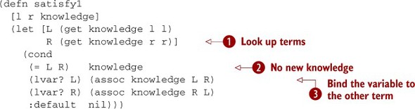
The function satisfy1 starts by attempting to build knowledge about the potential equality of two terms. It does this by first using the existing knowledge about the terms (or the terms themselves, if no existing knowledge is found in the lookup) . You require a Clojure map as the final argument for the sake of simplicity, but that requirement will need adjustment in the next section.

Moving on, you assume that if the terms are equal, you want to return the existing knowledge . By not adding any binding to the map, you effectively say that the terms are already equal. For example, how do you satisfy the equality of 1 and 1? Equality between the terms is already satisfied. Returning the existing knowledge allows you to chain satisfy1 calls for the purpose of gradually satisfying high-order relationships (shown in a moment).

If either term is a variable, the way to satisfy it is to set the binding from the variable term to the other term . This flip-flop action on the variable binding is a simple yet elegant solution to satisfying variable terms. Although returning nil at the end of the cond isn’t strictly necessary, it helps to clarify that by default, two terms aren’t satisfiable.

Here are two calls:

(satisfy1 '?something 2 {})
;;=> {?something 2}

(satisfy1 2 '?something {})
;;=> {?something 2}

In both cases, the results say that in order to satisfy equality of the number 2 and the variable ?something, the latter must equal 2. This is so intuitive that it hardly bears mentioning; but the subtlety of unification in general is shown with the following call:^[3]

³ Unification is a surprisingly rich topic of exploration, and we’ve barely begun to scratch the surface. Our introduction should be enough to get you through this chapter. If you’d like to learn more, feel free to petition Manning for a book on logic programming.

(satisfy1 '?x '?y {})
;;=> {?x ?y}

This is more subtle. The result of satisfy1 in this case states that to achieve the equality of two variables, one variable must equal the other. This condition is what makes unification different than something like destructuring or even pattern matching.^[4] By allowing variables to occupy the solution, you can defer satisfying the equality until further knowledge becomes available. For example, if you know that satisfying equality of two variables requires that one equal the other, whatever their value, then you can fully satisfy the terms by supplying a value:

⁴ Although unification can be thought of as two-way pattern matching.

(->> {}
     (satisfy1 '?x '?y)
     (satisfy1 '?x 1))

;;=> {?y 1, ?x ?y}

You can see that if ?x equals ?y and ?y equals 1, then ?x equals 1 also. Your first attempt at solving satisfiability can’t make this kind of inference, but with a few modifications you can make it do so.

Satisfying seqs

Observe the following:

(= '(1 2 3) '(1 2 3))

You would expect this expression to evaluate to true, and your expectation would be met. Likewise, the expression (= '(1 2 3) '(100 200 300)) results in false. (1 2 3) and (100 200 300) aren’t equal to each other, nor could they ever be. But conceptualize the following:

(= '(1 2 3) '(1 ?something 3))

You might say that, as in the previous section, the equality check will pass or fail depending on the value of ?something. In some books on functional or logic programming, the authors try to draw a connection between programming logic and mathematical logic. The reason is that there is a connection: one only hinted at by our use of the word variable to represent an unknown value in a vector.^[5] In algebra class, you might have seen problems of this form:

⁵ Usually, first-order (or maybe higher-order) logic with universal or existential quantifiers is considered the philosophical motivation for logic programming. Although our algebra example isn’t of the same nature, it can be encoded in first-order logic.

What is the value of x in the term:

38 - (x + 2) = 5x

We won’t make you break out your paper and pencil—the answer to this formula is x = 6. The variable x is in effect the same as our notion of a variable ?something.

To satisfy the equality of the two seqs (1 2 3) and (1 ?something 3), the binding of ?something would have to be equal to the number 2. But satisfy1 from the previous section won’t help you derive that information. Instead, you need to modify the algorithm as shown next, to account for nested variables and recursive definitions.^[6]

⁶ In most of the literature on logic programming, our function satisfy is called unify.

Listing 16.5. Function that satisfies seqs

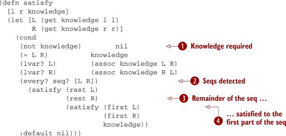
Although basically the same shape as satisfy1, the new function satisfy has two additions that extend it. First, because the definition is recursive, you can no longer assume knowledge is given. Because the default case returns nil, you can use that fact as the terminating condition for failure . But this is a minor change compared to the recursive calls themselves. The point is easy to elucidate: when both terms are seqs, you want to attempt to satisfy them as deeply as they go . This is accomplished by building the knowledge of the first elements in each seq and using that as a seed for then satisfying the rest of the seqs . This is where the advantage of adding to the knowledge comes in handy: satisfy uses knowledge it learned earlier to resolve bindings later in the process. Observe the following:

(satisfy '(1 2 3) '(1 ?something 3) {})
;;=> {?something 2}

This, as we discussed earlier, is the binding that makes the two seqs equal. It doesn’t matter how deeply nested the variables are:

(satisfy '((((?something)))) '((((2)))) {})
;;=> {?something 2}

Nor does it matter how scattered the variables happen to be:

(satisfy '(?x 2 3 (4 5 ?z))
         '(1 2 ?y (4 5 6))
         {})

;;=> {?z 6, ?y 3, ?x 1}

(satisfy '?x '(?y) {})
;;=> {?x (?y)}

The new function satisfies the terms when possible:

(satisfy '(?x 10000 3) '(1 2 ?y) {})
;;=> nil

Using a simple recursive algorithm (let’s call it a data-programmable engine), you can derive a specific kind of knowledge from two pieces of data: the variable bindings required to make them equal. There is a hard limit to how far this knowledge takes you, though. On its own, deriving bindings is of limited use. But you can take that knowledge and build on it to form more complex functions.

16.2.2. Substitution

The satisfy function can return a map representing variable bindings. You can view those bindings as an environment providing a context for substituting holes in a template for actual values. The function that fulfills this substitution, named subst, is defined in the following listing.

Listing 16.6. Walking a data structure and substituting logic variables for bound values

(require '[clojure.walk :as walk])
(defn subst [term binds]
  (walk/prewalk

   (fn [expr]
     (if (lvar? expr)
       (or (binds expr) expr)
       expr))
   term))

The function subst uses Clojure’s tree-traversal library clojure.walk to examine each element in turn, attempting to replace it with its value binding if it’s a logic variable. You can see subst in action here:

(subst '(1 ?x 3) '{?x 2})
;;=> (1 2 3)

(subst '((((?x)))) '{?x 2})
;;=> ((((2))))

(subst '[1 ?x 3] '{?x 2})
;;=> [1 2 3]

(subst '{:a ?x, :b [1 ?x 3]} '{?x 2})
;;=> {:a 2, :b [1 2 3]}

And here’s how subst acts when given incomplete knowledge (bindings):

(subst '(1 ?x 3) '{})
;;=> (1 ?x 3)

(subst '(1 ?x 3) '{?x ?y})
;;=> (1 ?y 3)

The beauty of using the clojure.walk library is that it preserves the original type of the target, as shown. You could imagine a web-templating system built on something like subst:

(def page
  '[:html
    [:head [:title ?title]]
    [:body [:h1 ?title]]])

(subst page '{?title "Hi!"})
;;=> [:html [:head [:title "Hi!"]] [:body [:h1 "Hi!"]]]

But the reason we mention it is that it serves as the basis for the unification of two terms.

16.2.3. Unification

The term unification is defined as a function that takes two terms and unifies them in the empty context, finally returning a new substitution. For practical purposes, unification is composed of three separate and orthogonal functions:

Deriving a binding as defined in satisfy
Substitution as defined in subst
Melding two structures together as defined shortly in meld

Based on what we’ve shown so far, you’ve created two of the tools needed to perform the unification suite. The missing tool, meld, takes two seqs and melds them together, taking into account all embedded logic variables.

Listing 16.7. Melding two seqs, substituting logic variables

(defn meld [term1 term2]
  (->> {}
       (satisfy term1 term2)
       (subst term1)))

meld derives the bindings in play between two seqs and then uses those bindings to perform a substitution on either one. Although it’s not a comprehensive solution, it can handle a fair amount of melds, including many with relative bindings:

(meld '(1 ?x 3) '(1 2 ?y))
;;=> (1 2 3)

(meld '(1 ?x) '(?y (?y 2)))
;;=> (1 (1 2))

Throughout this chapter, you’ve built up gradually more complex, yet declarative functions using nothing but data and the bare minimum of program logic. In every case, from satisfy to subst to meld, you’ve implemented tiny data-programmable engines and supplied them with data to see how they worked. Likewise, you built one on the other to create higher-level functionality; each in turn its own data-programmable engine. But although unification is interesting and useful for various problems, as a model for declarative computation it’s left wanting.

A powerful feature of unification that nevertheless causes issue is shown next:

(satisfy '?x 1 (satisfy '?x '?y {}))
;;=> {?y 1, ?x ?y}

(satisfy '(1 ?x) '(?y (?y 2)) {})
;;=> {?x (?y 2), ?y 1}

In these examples, variables are retained in the answer (there are non-ground terms). Although you can probably see that in both cases, ?y is 1, the algorithm can’t. Therefore, you need to take this process a step further.

Simple unification unfortunately only gets you so far. On its own, it’s not enough to solve even a simple algebraic expression:

What is the value of x in the term:

5x - 2(x - 5) = 4x

Instead, you need some kind of operational logic to solve general-purpose problems in a declarative fashion. Fortunately, the Clojure contrib library provides a tool called core.logic that builds on the principles of unification to move us closer to a declarative ideal.

16.3. An introduction to core.logic

In this book, we’ve tried hard to maintain a strict policy of highlighting core Clojure functions and features. But one Clojure-contrib library has grabbed not only our attention and imagination but also those of the Clojure community as a whole. The library, called core.logic, provides a system of operational logic for making general inferences using the principles of unification. This section covers the basics of core.logic including some examples.

First, to use core.logic, you need to include it in your project dependencies (or see the example in the preface) in your preferred way and add the following declaration to a namespace for use:

(ns joy.logic.cl
  (require [clojure.core.logic :as logic]))

From here, you have access to core.logic’s features.

16.3.1. It’s all about unification

Previously in this chapter, you created a simplified unification system out of three functions: satisfy, subst, and meld. Of particular importance is the satisfy function. Recall how satisfy works:

(satisfy '?answer 5 {})
;;=> {answer 5}

The satisfy function attempts to answer this question: How can two terms be made equal? Surprisingly, this simple question forms the basis for much of what is commonly known as logic programming. Before diving deeper into that particular point, it’s worth noting that the core.logic library contains a goal constructor named == that isn’t the same as clojure.core/==. Mimicking the action of satisfy using core.logic’s == is as follows:

(logic/run* [answer]
  (logic/== answer 5))
;;=> (5)

The run* form provides a lexical binding [answer] that declares the logic variables in context for the forms nested within. Likewise, the answer logic variable, because it’s bound by the run* form, represents the final result. The == unifier looks similar to the satisfy call, except that the context map is implicit rather than supplied as an argument. The return value (5) maps one for one with the established binding [answer]. To see how multiple bindings are established, observe the following:

(logic/run* [val1 val2]
  (logic/== {:a val1, :b 2}
            {:a 1,    :b val2}))

;;=> ([1 2])

This is already more powerful than satisfy: although satisfy only unifies with scalars and lists, core.logic unifies against all Clojure’s data types.^[7] This ability obviates the need to continue with satisfy. Like satisfy, logic/== can leave logic variables in its wake:

⁷ Additionally, core.logic provides mechanisms for unifying against arbitrary types including Java objects! This capability is sadly outside the scope of this chapter.

(logic/run* [x y]
  (logic/== x y))

;;=> ([_0 _0])

The binding represented by _0 is a logic variable (like ?x in satisfy), and core.logic represents logic variables using an underscore followed by unique numbers. In the previous case, the dual-variable binding states: in order for x and y to be equal, they must both be the same unknown value.

Another example of unification in core.logic is the case where unification fails:

(logic/run* [q]
  (logic/== q 1)
  (logic/== q 2))

;;=> ()

Two attempted unifications against the same logic variable q fail unification because the logic variable’s binding can’t be both 1 and 2 at the same time. But core.logic provides another form called conde that attempts to unify terms in multiple universes:

(logic/run* [george]
  (logic/conde
   [(logic/== george :born)]
   [(logic/== george :unborn)]))

;;=> (:born :unborn)

The conde form takes any number of forms inside the [], and it can contain multiples. In the previous example, the bindings represent the value of george in two different universes, one where he is born and another where he isn’t born.^[8]

⁸ As in the Frank Capra film It’s a Wonderful Life, starring Jimmy Stewart.

An interesting aspect of core.logic is that, although it utilizes unification, it provides an operational system of logic called miniKanren^[9] (Friedman 2006) embedded right inside Clojure. With the inclusion of conde, core.logic provides a way of reasoning about unification along different parameters aside from attempting to make two terms equal. Before diving into solving problems with core.logic, let’s take a few moments to cover the information model core.logic uses: relational data.

⁹ MiniKanren is a system of logic classified as relational logic programming.

16.3.2. Relations

In common database terminology, a relation is a group of related properties (often called tuples). The best way to explain a tuple is to think about things in reality that are related. For example, planets are related to stars in that they often orbit around them. Therefore, a useful relation for describing orbits could be aptly named orbits. The core.logic library has a macro defrel that you use to define the structure of relations:

(ns joy.logic.planets
  (require [clojure.core.logic :as logic]))

(logic/defrel orbits orbital body)

The relation orbits contains two attributes: orbital (the thing that orbits: Earth) and body (the thing that is orbited around: Sun). Defining data for the orbits relation is done via the fact macro:

(logic/fact orbits :mercury :sun)
(logic/fact orbits :venus   :sun)
(logic/fact orbits :earth   :sun)
(logic/fact orbits :mars    :sun)
(logic/fact orbits :jupiter :sun)
(logic/fact orbits :saturn  :sun)
(logic/fact orbits :uranus  :sun)
(logic/fact orbits :neptune :sun)

Each of these logic/fact calls describes a single tuple in the relation orbits. A tuple is a grouping of named properties. In the case of the orbits relation, the tuples can be imagined logically laid out as vectors of the following form:

'[orbits :mercury :sun]

; ...

'[orbits :neptune :sun]

In these vectors, the entries can be said to align with the property names:

The relation tag orbits
The orbital tag (:mercury)
The body tag (:sun)

Seems pretty simple right? Table 16.1 presents this information in a tabular way.

Table 16.1. `Planets` table

ID	Planet	Orbits
1	Mercury	Stars[1]
2	Venus	Stars[1]
3	Earth	Stars[1]
4	Mars	Stars[1]
5	Jupiter	Stars[1]
6	Saturn	Stars[1]
7	Uranus	Stars[1]
8	Neptune	Stars[1]

This table is laid out in a way that hearkens to something you might see describing a relational database table. Specifically, the ID fields and especially the Stars[1] entries refer to the way keys relate one set of properties to another. In the case of the Orbits link, it might logically point to an entry in table 16.2.

Table 16.2. `Stars` table

ID	Star
1	Sun
2	Alpha Centauri

In the case of the orbits core.logic relation, a planet is related to a star because the same name :sun is used to refer to the same star in all the tuples forming the orbits relation. This is subtly different from the way traditional relational databases link entries together explicitly via ID chains. In a relational scheme like that used in core.logic, links between relations are derived via symbolic matching. We’ll show what this means in the next section.

Querying the orbits relation

Now that we’ve explained relations in excruciating detail, we’ll turn our attention to how core.logic is used to form queries over relations. If you’ll recall, you initiate a call to core.logic using the run* command. In the body of the run* call, you use the unification operator == to satisfy variable bindings and retrieve answers. In the case of querying the orbits relation, you’ll do likewise, but you’ll rearrange things a bit and use a new core.logic operator: fresh. Without further ado, a query to find all the planets that orbit anything is shown in the following listing.

Listing 16.8. Querying planetary bodies

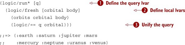
The form of this query looks similar to what you’ve seen so far, except for a few significant differences. The first major difference is that you bind a single name in the run* call q. You’ll see this a lot in core.logic programs. Using q at the outermost level basically states that q is the overall query result . To isolate the logic variables used to perform the query, you use the fresh macro, which works similarly to Clojure’s let form. The fresh macro declares scoped logic variable names for use in enclosed goals . Additionally, any goals aggregated within fresh are grouped together to form a logical conjunction (logical and). In other words, both the fact (orbits orbital body)and the unification (logic/== q orbital) should be satisfied for the entire body of fresh to be considered satisfied. If either fails, then the conjunction as a whole fails.

This example uses the names orbital and body, which happen to correspond to the orbits property tags, but you could just as easily use o and p instead. The purpose of fresh is to declare logic variable names used as holes to be satisfied via unification within the subgoals (nested goals grouped together to form larger goals) and to logically group those goals via conjunction. Finally, unifying the orbital logic variable with the query variable q returns all bindings with a value in the orbital property—which of course are all the planets in our solar system.^[10]

¹⁰ We’re not really Pluto haters—please don’t judge us.

16.3.3. Subgoals

A subgoal in core.logic is a way to aggregate common matches under a common name for the purposes of drawing logical data connections, without needing to lift connections into data explicitly. Imagine if you wanted to rewrite the original query that listed all the planets. The original query uses the idea that anything that orbits anything else is a planet. You can encapsulate that idea in a subgoal planeto, or a function that takes a relation and returns a relation:

(logic/defrel stars star)

(logic/fact stars :sun)
(defn planeto [body]
  (logic/fresh [star]
    (stars star)
    (orbits body star)))

Note

By convention, functions that take a core.logic relation as input end with the letter o, as in the definition we just presented.^[11]

¹¹ If you cross your eyes, the o looks like a degree symbol: the traditional ending to relational functions in mini-Kanren. If you cross your eyes a little more, the degree symbol looks like a question mark, just as Dr. Friedman would like it.

The planeto subgoal provides a way to jack in to the core.logic inference engine to offer discrete chunks of inferencing, often referred to as rules or axioms. In the case of planeto, the rule states that something is a planet if it orbits a star. You facilitate this subgoal by creating a new relation defining stars. We know that not everything that orbits a star is a planet, but for the sake of illustration we’ll make that assumption here. Now, if you plug the use of planeto into run*, you should get some interesting results:

(logic/run* [q]
  (planeto :earth))

;;=> (_0)

Attempting to ask the query, “Is :earth a planet?” returns a logic variable. If you recall from our previous discussion, the return of a logic variable means the query is sound but there was no unification. In this case, you can unify q with a value to see a different result:

(logic/run* [q]
  (planeto :earth)
  (logic/== q true))

;;=> (true)

So the answer to “Is :earth a planet?” according to the rule defined by planeto is true. You can attempt to ask the same question of :sun:

(logic/run* [q]
  (planeto :sun)
  (logic/== q true))

;;=> ()

As shown, the query states that indeed, :sun isn’t a planet. To show one more example of planeto, you can use it to show all the planets in your fact-base:

(logic/run* [q]
  (logic/fresh [orbital]
    (planeto orbital)
    (logic/== q orbital)))

;;=> (:earth :saturn :jupiter :mars
;;    :mercury :neptune :uranus :venus)

You can augment the current fact-bases by adding new facts and running the same queries to see how the answers change:

(logic/fact stars :alpha-centauri)
(logic/fact orbits :Bb :alpha-centauri)

(logic/run* [q]
  (planeto :Bb))

;;=> (_0)

The good news is that adding a new star and one of its orbitals resolves exactly the way you expect. And of course, running the original query again does too:

(logic/run* [q]
  (logic/fresh [orbital]
    (planeto orbital)
    (logic/== q orbital)))

;;=> (:earth :saturn :jupiter :mars :Bb
;;    :mercury :neptune :uranus :venus)

As shown, the idea of planet-ness exists nowhere in either of your fact-bases. But the notion of planet-ness can be derived from the data as a result of the relationships between relations and their properties.

The satelliteo subgoal

It turns out that planets can orbit things other than stars. But when a planet orbits another planet, it’s called a satellite rather than a planet. You can add the notion of satellite-ness to the example relational model via table 16.3.

Table 16.3. `Satellites` table

ID	Satellite	Planet
1	Moon	Planet[3]
2	Phobos	Planet[4]

But now you’ve separated the idea of satellite from planet; and although there is a logical difference, they aren’t really different because satellites are still planets. Therefore, you could jam the satellites into the Planets table and instead implement the Satellites table to contain links only, as shown in table 16.4.

Table 16.4. `Satellites` table implemented as links

Satellite	Planet
Planet[9]	Planet[3]
Planet[10]	Planet[4]

The problem with this scheme is that the idea of satellite-ness has been lifted into the realm of data, where it’s just a logical distinction. Where symbolic logical programming shines is that logical distinctions can be expressed in terms of subgoals.

A subgoal similar to, but slightly more complicated than, planeto is satelliteo:

(defn satelliteo [body]
  (logic/fresh [p]
      (orbits body p)
      (planeto p)))

The subgoal satelliteo uses the existing subgoal planeto to state that a planet is a satellite if: 1) it orbits something and 2) the thing it orbits is a planet.

The interesting aspect of informally stating the behavior of satelliteo in words is that you impose an ordering of clauses. But core.logic is under no such constraints. You could swap the check of (orbits body p) and (planeto p), and the subgoal would work the same. Here it is in action:

(logic/run* [q]
  (satelliteo :sun))

;;=> ()

(logic/run* [q]
  (satelliteo :earth))

;;=> ()

As you might expect, neither :sun nor :earth is a satellite according to the rules of satelliteo. In fact, none of the facts in your fact-bases constitute logical satellites, so you need to add one:

(logic/fact orbits :moon :earth)

Now the check of satelliteo should pass:

(logic/run* [q]
  (satelliteo :moon))

;;=> (_0)

We’ve shown you how to use run*, fresh, ==, and subgoals. You’re ready to begin forming your own inferences using core.logic.

Closed-world principle

Let’s add a few more data points:

(logic/fact orbits :phobos :mars)
(logic/fact orbits :deimos :mars)
(logic/fact orbits :io :jupiter)
(logic/fact orbits :europa :jupiter)
(logic/fact orbits :ganymede :jupiter)
(logic/fact orbits :callisto :jupiter)

(logic/run* [q]
  (satelliteo :io))
;;=> (_0)

Adding a smattering of new orbitals allows you to infer more data for your existing goals. But imagine if you attempted to ask the following perfectly legitimate query:

(logic/run* [q]
  (orbits :leda :jupiter))
;;=> ()

Perhaps this is no surprise, because you created facts about only 4 of Jupiter’s 67 moons, not including Leda. But this result points to the closed-world nature of core.logic inferencing. A closed-world system is one that makes inferences under the assumption that every fact available to it represents the entire set of knowledge in the “world.” Even though Leda is in reality a satellite of Jupiter, it isn’t, according to this query, because in the closed world of the core.logic fact-base there is no such fact nor any way to derive that information. The converse to the closed-world principle is the open-world principle, which states that any query is assumed to be unknown if it can’t be derived.

In the next section, we’ll talk about the idea that although core.logic is a powerful logic-programming system, it’s a little too open-ended.

16.4. Constraints

In this final section on logic programming, we’ll explore the way that, by itself, the core.logic search facilities are too open-ended. Even though core.logic’s search is still more directed than a brute-force solver, it could be more directed given a finer-grained degree of specification. We’ll talk first about the notion of constraint programming and core.logic’s capabilities supporting it.

16.4.1. An introduction to constraint programming

When we begin to discuss constraint logic programming, it’s worth taking a step back and drawing analogies. Take the following definition of a function called doubler:

(defn doubler [n] (* n 2))

Because of the dynamic nature of Clojure’s type system, the doubler function isn’t constrained in any way in the types of arguments it takes:

(doubler 2)
;;=> 4

(doubler Math/E)
;;=> 5.43656365691809

(doubler 38781787272072020703083739N)
;;=> 77563574544144041406167478N

(doubler 1/8)
;;=> 1/4

But with the good comes the bad. The doubler function will happily take absolutely any value:

(doubler [])
;; ClassCastException ...

(doubler #(%))
;; ClassCastException ...

(doubler "")
;; ClassCastException ...

You get the idea. Although a Clojure function can take any value as an argument, doing so may not make logical sense. Therefore, in chapter 8 you created a defcontract form that allowed you to define input and output constraints on functions, which were checked at runtime:

(def doubling
  (defcontract c [x]
    (require (number? x))
    (ensure  (= % (* 2 x)))))

This contract states that as long as a function receives a number, it will return that number doubled. Otherwise an AssertionError will occur:

(def checked-doubler (partial doubling doubler))

(checked-doubler "")
;; AssertionError: Assert failed: (number? x)

The doubling contract constrains the legal input types taken on by the argument to the doubler function.

In much the same way, you can view the unification of a logic variable with a function parameter. Observe the following:

(logic/run* [q]
   (logic/fresh [x y]
     (logic/== q [x y])))

 ;;=> ([_0 _1])

The result ([_0 _1]) states that the query variable q will unify with the vector [x y] as long as x and y are, well, anything:

(logic/run* [q]
  (logic/fresh [x y]

    (logic/== [:pizza "Java"] [x y])
    (logic/== q [x y])))

;;=> ([:pizza "Java"])

But core.logic provides a simple operator != that allows you to define “dis-equality” constraints on a logic variable. Plugging the use of != into the previous simple query yields this:

(logic/run* [q]
  (logic/fresh [x y]
    (logic/== q [x y])
    (logic/!= y "Java")))

;;=> (([_0 _1] :- (!= (_1 "Java"))))

This is certainly an odd-looking result, but it makes sense once you know how it’s constructed. The first part, [_0 _1], states the same thing as before: x and y can be anything. But the next segment describes the constraint that the variable _1 can’t equal "Java". In other words, x and y can be anything, as long as y isn’t "Java". You can prove this by plugging the constraint into this larger query:

(logic/run* [q]
  (logic/fresh [x y]
    (logic/== [:pizza "Java"] [x y])
    (logic/== q [x y])
    (logic/!= y "Java")))

;;=> ()

Because y is constrained to never take on the value "Java", attempting to unify a term where such a value is present causes the unification to fail. You can make unification succeed by attempting a different value instead:

(logic/run* [q]
  (logic/fresh [x y]
    (logic/== [:pizza "Scala"] [x y])
    (logic/== q [x y])
    (logic/!= y "Java")))

;;=> ([:pizza "Scala"])

Although it’s useful to limit the values a logic variable can take on via the dis-equality operator !=, its use only works to slightly limit a near-limitless range of values. There are further ways to constrain the values by defining the bounds of possible values, called finite domains.

16.4.2. Limiting binding via finite domains

Similar to the way the doubler function takes any possible value, the following query allows any possible value unification:

(logic/run* [q]
  (logic/fresh [n]
    (logic/== q n)))

;;=> (_0)

As shown in the previous section, you can constrain such queries using the dis-equality constraint !=:

(logic/run* [q]
  (logic/fresh [n]
    (logic/!= 0 n)
    (logic/== q n)))

;;=> ((_0 :- (!= (_0 0))))

But how can you instead constrain the unification to exclude negative numbers? The core.logic library provides a way to express such a constraint using its finite-domain constraint system, which is located in the clojure.core.logic.fd namespace:

(require '[clojure.core.logic.fd :as fd])

The finite-domain namespace provides a number of functions to constrain logic binding, including +, -, *, quot, ==, !=, <, <=, >, >=, in, interval, domain, and distinct. Among these options, the in and interval constraints seem promising for realizing the aforementioned constraint:

;; CAUTION: RUN THIS AT YOUR OWN RISK
(logic/run* [q]
  (logic/fresh [n]
    (fd/in n (fd/interval 1 Integer/MAX_VALUE))
    (logic/== q n)))

;;=> (1 2 3 ... many more numbers follow)

The fd/in macro states that the logic variable n is constrained to fall within certain values or intervals. For example, you can tighten the range using the fd/domain macro as follows:

(logic/run* [q]
  (logic/fresh [n]
    (fd/in n (fd/domain 0 1))
    (logic/== q n)))

;;=> (0 1)

The fd/in macro always takes a domain as the last argument, with possible values within that domain preceding it. Here’s a way to enumerate all the possible combinations for tossing two consecutive coins:

(logic/run* [q]
  (let [coin (fd/domain 0 1)]
    (logic/fresh [heads tails]
      (fd/in heads 0 coin)
      (fd/in tails 1 coin)
      (logic/== q [heads tails]))))

;;=> ([0 0] [0 1] [1 0] [1 1])

The result matches our intuition: heads/heads, heads/tails, tails/heads, or tails/tails. But we can go deeper than this; as it happens, the use of a finite domain matches closely with the problem that started this chapter, Sudoku solving.

16.4.3. Solving Sudoku with finite domains

As we said earlier in the chapter, when we enumerated the rules of Sudoku, the following constraints are imposed on the solutions to a puzzle:

Each column must contain one occurrence of each digit from 1–9.
Each row must contain one occurrence of each digit from 1–9.
Each 3 × 3 subsection must contain one occurrence of each digit from 1–9.

Something that should jump out in those descriptions is the range 1–9. That a range is involved points to a finite domain. Indeed, any given cell must fall within (domain 1 9). But before we dive in to solving Sudoku with core.logic, some parts could be simplified from the previous attempt using the brute-force solver.

For example, the brute-force solver worked by placing mostly random, yet legal, values on the board one square at a time. Although a core.logic solver will operate somewhat the same way, the placement is internal and driven by the constraint rules. Therefore, you need to adjust the new solver to operate over three different structures: row, column, and subgrid sequences. To start, the following function implements the logic to create a sequence of all the rows on a Sudoku board:

(defn rowify [board]
  (->> board
       (partition 9)
       (map vec)
       vec))

Observe how rowify works on the original puzzle b1:

(rowify b1)

;;=> [[3 - - - - 5 - 1 -]
      [- 7 - - - 6 - 3 -]
      [1 - - - 9 - - - -]
      [7 - 8 - - - - 9 -]
      [9 - - 4 - 8 - - 2]
      [- 6 - - - - 5 - 1]
      [- - - - 4 - - - 6]
      [- 4 - 7 - - - 2 -]
      [- 2 - 6 - - - - 3]]

The row view is multipurpose, serving as a structure for further processing. Another function colify operates on the row view to build the columns:

(defn colify [rows]
  (apply map vector rows))

The use of colify is as follows:

(colify (rowify b1))
;;=> ([3 - 1 7 9 - - - -] [- 7 - - - 6 - 4 2] ... )

Finally, creating a subgrid view is trickier, but it can be solved with nested for comprehensions:

(defn subgrid [rows]
  (partition 9
    (for [row (range 0 9 3)
          col (range 0 9 3)
          x (range row (+ row 3))
          y (range col (+ col 3))]
      (get-in rows [x y]))))

The subgrid function is an indexer that walks the rows structure: it plucks out each element in every subgrid, starting from the top-left and moving down from left to right. The result of a call to subgrid is as follows:

(subgrid (rowify b1))

;;=> ((3 - - - 7 - 1 - -) (- - 5 - - 6 - 9 -) ... )

These subgrid views align with the subgrids shown back in figure 16.1. But in order to work with a Sudoku board within the confines of the core.logic system, you won’t work directly on the numbers and empty slots. Instead, you’ll preprocess the board so the cells are logic variables. You can create a function logic-board that initializes a completely empty Sudoku-sized board filled with logic variables:

(def logic-board #(repeatedly 81 logic/lvar))

The logic-board function yields an 81-cell (9 × 9) flat Sudoku board filled with uninitialized logic variables. A logic variable can take on any value via unification, as we’ve shown throughout this chapter. But you need a way to initialize the cells containing logic variables with corresponding number hints in the initialization board. The natural way to perform this initialization is to unify the number hint with the corresponding logic variable. You can do this recursively, as shown in the following listing.

Listing 16.9. Recursively initializing a Sudoku board filled with logic variables

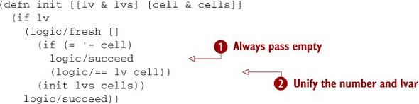
On the surface, the init function looks like a normal recursive walk of two sequences. Although this is true, the reality of its action is subtle and bears explanation. To start, the use of fresh with no bindings serves only to aggregate subgoals. The first subgoal is one of two choices. First, if the value in a given board cell is the symbol -, the goal is considered successful by default . On the other hand, if the cell contains any other value, then the corresponding logic variable is unified with that value . The purpose of init is to bind known number values to certain logic variables, as shown here:

-------------------------------------
| 3   ?   ? | ?   ?   5 | ?   1   ? |
| ?   7   ? | ?   ?   6 | ?   3   ? |
| 1   ?   ? | ?   9   ? | ?   ?   ? |
-------------------------------------
| 7   ?   8 | ?   ?   ? | ?   9   ? |
| 9   ?   ? | 4   ?   8 | ?   ?   2 |
| ?   6   ? | ?   ?   ? | 5   ?   1 |
-------------------------------------
| ?   ?   ? | ?   4   ? | ?   ?   6 |
| ?   4   ? | 7   ?   ? | ?   2   ? |
| ?   2   ? | 6   ?   ? | ?   ?   3 |
-------------------------------------

The initialized board becomes important when you reuse the same logic variables to form the row-, column-, and subgoal-view sequences in the following listing.

Listing 16.10. A core.logic Sudoku solver

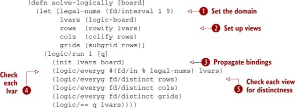
We’re not sure about you, but we find it breathtaking that a Sudoku solver can be described in 12 lines of Clojure code. The key to its functionality lies in a few interrelated factors. First, establishing the domain of each logic variable to fall within the range (fd/interval 1 9) is a direct transcription of the constraints described in the rules of Sudoku . The rowify, colify, and subgrid functions are used to build different views of the Sudoku cells while sharing common logic variables . Because the logic variables are shared, initializing certain logic variables with the number hints propagates the bindings to all shared views . The core.logic everyg function takes a function containing a subgoal and checks that each element succeeds that goal. The first case where everyg is used checks that the lvar bindings fall within the legal range . This check not only ensures that you’re given a legal seed board but also constrains every logic variable binding to fall within the domain. The fd/distinct function is applied across each logical view (rows, columns, and subgrids) to check that the domain is adhered to and that each grouping contains unique values . Striving for distinctness in each view’s components drives the core.logic search to an eventual solution:

(-> b1
    solve-logically
    first
    prep
    print-board)

;; -------------------------------------
;; | 3   8   6 | 2   7   5 | 4   1   9 |
;; | 4   7   9 | 8   1   6 | 2   3   5 |
;; | 1   5   2 | 3   9   4 | 8   6   7 |
;; -------------------------------------
;; | 7   3   8 | 5   2   1 | 6   9   4 |
;; | 9   1   5 | 4   6   8 | 3   7   2 |
;; | 2   6   4 | 9   3   7 | 5   8   1 |
;; -------------------------------------
;; | 8   9   3 | 1   4   2 | 7   5   6 |
;; | 6   4   1 | 7   5   3 | 9   2   8 |
;; | 5   2   7 | 6   8   9 | 1   4   3 |
;; -------------------------------------

You use logic/run 1 to perform the logic query and find only one solution.^[12] Well-designed Sudoku boards have only one solution, but many starting boards have more than one (Norvig 2011). We leave as an exercise for you an exploration of the vagaries of Sudoku. And core.logic is a wonderful vehicle for such an exploration.

¹² Whereas the brute-force solver takes on the order of seconds to calculate the same board position, the constraint-logic solution takes on the order of milliseconds.

The core.logic rabbit hole runs much deeper than we’re able to show in a single chapter, but we hope that, given a taste, you’ll further explore the wonders of logic programming.

16.5. Summary

This concludes our chapter on thinking code using logical programming techniques and the core.logic library. Although there are other ways to write a Sudoku solver more efficient than our brute-force solver, we attempted to draw a balance between functional and declarative techniques. Leading up to our discussion of the core.logic contributor library, we took a detour into a discussion of unification that provides a way to pattern-match structures containing variables. As a building block of the core.logic system, unification was a natural way to transition into the workings of the system, including facts, goals, subgoals, and the various functions and macros that provide those. Although core.logic can provide a convenient and powerful in-memory database query language, as shown with the planets example, you also saw how to use it to perform calculations. Along these lines, we explained how such calculations can be made more efficient by using constraints and finite domains to reduce the search space.

If you’re unaccustomed to writing logic programs with systems like core.logic, this chapter has likely exposed you to a different way of thinking about programs. We’ve found that Clojure has motivated us to think differently about building programs via its internal “why” and “how” and libraries like core.logic. In the next and final chapter of the book, we’ll share some of the ways Clojure has helped us look at problems and their solutions in new ways.

..................Content has been hidden....................

You can't read the all page of ebook, please click here login for view all page.

Table of Contents for Chapter 16. Thinking programs

Create new playlist

Sign In

Sign Up

Chapter 16. Thinking programs

16.1. A problem of search

16.1.1. A brute-force Sudoku solver

Figure 16.1. Starting position of the example Sudoku board

Listing 16.1. Printing the starting position of a Sudoku board

The regions of a Sudoku board

The rules of Sudoku

Listing 16.2. Brute-force Sudoku solver

16.1.2. Declarative is the goal

16.2. Thinking data via unification

16.2.1. Potential equality, or satisfiability

Satisfying variables

Listing 16.3. Identifying logic variables

Listing 16.4. Simplified satisfiability function

Satisfying seqs

Listing 16.5. Function that satisfies seqs

16.2.2. Substitution

Listing 16.6. Walking a data structure and substituting logic variables for bound values

16.2.3. Unification

Listing 16.7. Melding two seqs, substituting logic variables

16.3. An introduction to core.logic

16.3.1. It’s all about unification

16.3.2. Relations

Table 16.1. Planets table

Table 16.2. Stars table

Querying the orbits relation

Listing 16.8. Querying planetary bodies

16.3.3. Subgoals

Note

The satelliteo subgoal

Table 16.3. Satellites table

Table 16.4. Satellites table implemented as links

Closed-world principle

16.4. Constraints

16.4.1. An introduction to constraint programming

16.4.2. Limiting binding via finite domains

16.4.3. Solving Sudoku with finite domains

Listing 16.9. Recursively initializing a Sudoku board filled with logic variables

Listing 16.10. A core.logic Sudoku solver

16.5. Summary

Table of Contents for
Chapter 16. Thinking programs

Table 16.1. `Planets` table

Table 16.2. `Stars` table

Table 16.3. `Satellites` table

Table 16.4. `Satellites` table implemented as links