
2
Applications of Equilibrium Thermodynamic Degradation to Complex and Simple Systems: Entropy Damage, Vibration, Temperature, Noise Analysis, and Thermodynamic Potentials
2.1 Cumulative Entropy Damage Approach in Physics of Failure
Entropy is an extensive property. If we isolate an area enclosing the system and its environment such that no heat, mass flows, or work flows in or out, then we can keep tabs on the total entropy (Figure 2.1).

Figure 2.1 The entropy change of an isolated system is the sum of the entropy changes of its components, and is never less than zero
In this case the entropy generated from the isolated area has
the total entropy of a system is equal to the sum of the entropies of the subsystems (or parts), so the entropy change is

We now can define here the Cumulative Entropy Damage Equation:

where, for the ith subsystem (see Equation (1.9)),
This seemingly obvious outcome (Equation (2.2)) is an important result not only for complex system reliability, but also for device reliability. This will be detailed throughout this chapter.
Note the non-damage entropy flow can go in or out depending on the process so it is possible for a subsystem’s entropy to decrease (become more ordered).
Often in reliability (when redundancy is not used), similar to Equation (2.2), the failure rate λ of the system is equal to the sum of the failure rate of its parts: ![]() .
.
In this case when any part fails, the system fails. Given that an ith subsystem’s entropy damage is increasing at a higher rate compared to the other subsystems, then it is dominating system-level damage. Therefore, the impeding failure of the ith subsystem is a rate-controlling failure of the system, and its rate of damage affects the system total entropy such that
If the resolution is reasonable, we can keep tabs on ΔSsystem damage over time by monitoring the rate controlling subsystem’s entropy damage. As long as we can somehow resolve the damage subsystem problem, that is,
Sensitivity of our measurement system for determining impending failure may likely depend on a part’s entropy damage resolution. This will be more obvious when we are describing noise analysis in Sections 2.5–2.9 and we are concerned about signal to noise issues. In this case, it is the noise rather than the signal that we will be looking at.
2.1.1 Example 2.1: Miner’s Rule Derivation
One basic example of how the important result of Equation (2.2) can be used is to help explain what is termed Miner’s fatigue rule, which is a key area in physics of failure.
Consider a subsystem that is made up of, say, metal with defect sites such as a cell lattice shown in Figure 2.2. Just as the entropy of each subsystem is the sum of the entropies, so too is the entropy damage for each cell C which adds up for a subsystem that is under some sort of stress such as cyclic fatigue, as shown in Figure 2.2. Suppose we have n damaged cells so the total entropy damage is

where n is the total number of cells with entropy damage Sdamage-cell,i. We assume equal entropy damage per cell. Consider that we have M total cells of potential damage to failure that would lead to a maximum cumulative damage Smax. Then the cumulative entropy damage can be normalized:
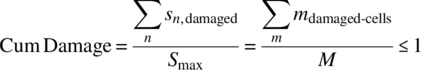
where sn is the entropy damage of the nth cell, and m represents a damaged cell such that Σm is the number of damaged cells observed.

Figure 2.2 Cell fatigue dislocations and cumulating entropy
If all the cells were damaged the entropy would be at a maximum, then the damage is equal to 1 and this should be equal to counting the number of damaged cells and dividing by the total number of cells that could cause failure. This is one way to measure damage. Here damage is assessed as a value between 0 and 1. Let’s assume that there is a linear relationship between the number of cells damaged and the number of fatigue cycles. Fatigue is also dependent on the stress of the cycle, for example, if we are bending metal back and forth, the stress level would be equal to the size of the bend. So for any ith stress level the number of cells damaged for n cycles is some stress fraction fi of the number of cycles:
Note that N is the number of cycles to failure and n is the number of cycles performed (N > n). Then we can write for the ith stress level:

When Damage = 1, failure occurs. This equation is called Miner’s rule [1]. Its accuracy then depends on the assumption of Equation (2.7). Furthermore, it follows that we can also invent here a related term called
When Damage = 1, the cumulative strength vanishes. Equation (2.7) turns out to be a good approximation, but it is of course not perfectly accurate. We do know that Miner’s rule is widely used and has useful validity. Miner’s rule is not just applicable to metal fatigue; it can be used for most systems where cumulative damage occurs. Later we have an example in Chapter 5 for secondary batteries. We have now derived it here using the cumulative entropy principle (Equation (2.2)). In Chapter 4 we provide a more accurate way to assess fatigue damage through the thermodynamic work principle.
2.1.2 Example 2.2: Miner’s Rule Example
Aluminum alloy has the following fatigue characteristics:
Stress 1, N = 45 cycles,
Stress 2, N = 310 cycles, and
Stress 3, N = 12 400 cycles.
How many times can the following sequence be repeated?
n 1 = 5 cycles at stress 1,
n 2 = 60 cycles at stress 2, and
n 3 = 495 cycles at stress 3
Solution
The fractions of life exhausted in each cycle type are:
The fraction of life exhausted in a complete sequence yields an approximate cumulative damage of 0.345 (with the cumulative strength decreasing down to 0.655). The life is entirely exhausted when damage D = 1 and has been produced 3 times when D = 1.035. The sequence can then be repeated about 2.9 times.
One interesting thing to note in fatigue damage is that even though damage accumulates with stress cycles, the degradation may not be easily detectable as the metal system is capable of performing its intended function as long as the system’s cumulative strength (Equation (2.9)) is greater than the stress that it is under. We typically find catastrophic failure occurs in a relatively short cycle time compared with the system’s cycle life. How then can we detect impending failure at such a mesoscopic level (mesoscopic is defined in Section 2.5)? One possible solution may be in what we term noise detection. This is discussed later in this chapter (see Sections 2.5–2.9).
2.1.3 Non-Cyclic Applications of Cumulative Damage
The thermodynamic second law requirement that
leads one to realize that even non-cyclic processes must cumulate damage. That is, we can write similar to Miner’s Rule, cumulative damage for non-cyclic time-dependent processes

where, by analogy with Miner’s cyclic rule, ti is the time of exposure of the ith stress level and τi is the total time to cause failure at the ith stress level. Not all processes age linearly with time as is found in Chapter 4, so the exponent P has been added for the generalized case where P is different from unity (see Chapter 4 for examples and Table 4.3). Equation (2.10) could be used for processes such as creep (0 < P < 1) and wear (P = 1) or even semiconductor degradation, any process where it might make sense to estimate the cumulative damage and/or the cumulative strength left (i.e., 1–Cum Damage). Note the time to failure does not have to be defined as a catastrophic failure. It may be prudent to apply this to parametric failure where τi then represents a parametric threshold time for failure. For example, τi could be the time when a certain strength, such as voltage output of a battery, degrades by 15%.
The main difference between a cyclic and non-cyclic process is that for a closed system undergoing a quasistatic cyclic process, the internal energy ΔU is often treated theoretically as unchanged in a thermodynamic cycle (see Section 3.3). This is a reversible assumption.
2.2 Measuring Entropy Damage Processes
To make degradation measurements, we need a repeatable method or process to make aging measurements at different times [2]. If we find that the entropy has changed over time from a repeatable quasistatic measurement process, then we are able to measure and track the aging that occurs between the system’s initial, intermediate, and final states. We can call this the entropy of an aging process. (Note that during system aging, we do not have to isolate the system. We only need to do this during our measurement process.)
We can theorize that any irreversible process that creates a change in entropy in a system under investigation can cause some degradation to the system. However, if we cannot measure this degradation, then in our macroscopic world the system has not actually aged. In terms of entropy generated from an initial and final state we have:
where the equal sign is for a reversible process and the inequality is for an irreversible process. However, what portion of the entropy generated causes degradation to the system and what portion does not? To clarify, similar to Equation (1.4) we have:
There is really no easy way to tell unless we can associate the degradation through a measurable quantity. Therefore, in thermodynamic damage, we are forced to define Sdamage in some measurable way.
As well in thermodynamics, we typically do not measure absolute values of entropy, only entropy change. Let us devise a nearly reversible quasistatic measurement process f, and take an entropy measurement of interest at time t1. Then:
The measurement process f must be consistent to a point that it is repeatable at a much later aging time t2. If some measurable degradation has occurred to our device, we can observe and record the entropy change:
Then we can determine if damage has occurred. If our measurement process f at time t1 and t2 is consistent, we should find a reasonable assessment of the entropy damage that has occurred between these measurement times to be:
where it equals zero if no device degradation is measurable. If we do generate some entropy damage during our measurement process (ti + Δti), it must be minimal compared to what is generated during the actual aging process between time t1 and t2. Then, our entropy measurement difference should be a good indication of the device aging/damage that is occurring between measurement times t1 and t2. The actual aging process to the system between time t1 and t2, might be a high level of stress applied to the system. Such stress need not be quasistatic. However, the stress must be limited to within reason so that we can repeat our measurement in a consistent manner at time t2. That is, the stress should not be so harsh that it will affect the consistency of the measurement process f.
One might for example have a device aging in an oven in a reliability test, then remove it and make a quasistatic entropy measurement f at time t1 and then put the device back in the oven later to do another measurement at time t2. Any resulting measurement difference is then attributed to entropy damage.
(Note that Equation (2.14) is a different statement from entropy flow which many books describe. Here we are concerned with entropy damage over a repeatable measurement process.)
2.3 Intermediate Thermodynamic Aging States and Sampling
In the above, our aging measurements were taken at an initial and final measurement time. These were quasistatic intermediate measurement states where little if any aging may have occurred. We are sampling the aging process. If the system had failed, it would have been in equilibrium with its environment. We did not track how the entropy of the aging process occurred over time. We were only concerned with whether or not degradation occurred. Our detection of the aging process is only limited by our ability to come up with a quasistatic measurement process. In theory, we can even detect if a complex rocket ship is degrading. Each measurement process takes place at a non-aging state at a key tracking point such as an initial, intermediate, or final measurement time. The measurement itself is taken in a small enough window of delta time to observe the state of the system but not cause any significant aging during our observation times.
Given a system, what quasistatic measurement process f will best detect degradation at an intermediate aging state? Part of the problem will always be resolution of our measurement process. Although we now have a tool that can possibly detect aging of a large system, can we make a measurement with enough resolution to observe its degradation? Can we take a partial sample in some way? For example, do we need to completely isolate the system and its environment in the entirety to make a measurement? We are now in a position which challenges our imagination.
The principals will therefore always be valid, but we may be limited by the practicality of the measurement. In the above case, the aging was associated with heat. Not all aging occurs in a manner that allows us to make degradation measurements in this way.
2.4 Measures for System-Level Entropy Damage
We next ask what state variables can be measured as an indicator at the system level for the entropy of aging. In this section we will explore the state system variables of temperature, and in Sections 2.5–2.9 system noise and system failure rate.
2.4.1 Measuring System Entropy Damage with Temperature
The most popular continuous intensive thermodynamic variable at the system level is temperature. In both mechanical and electrical systems, system internal temperature can be a key signature of disorder and increasing entropy. Simply put, if entropy damage increases, typically this is the result of some resistive or frictional heating process. Some examples will aid in our understanding of how such measurements can be accomplished with the aid of temperature observations.
2.4.2 Example 2.3: Resistor Aging
Resistor aging is a fundamental example, since resistance generates entropy. A resistor with value R ohms is subjected to environmental stress over time at temperature T1 while a current I1 passes through it for 1 month. Determine a measurement process to find the entropy at two thermodynamic non-aging states before the stress is applied and after it has been applied at times tinitial and tfinal, respectively. Determine if the resistor has aged from the measurement process and the final value for the resistor.
Before and after aging at temperature T1, we establish a quasistatic measurement process f to determine the entropy change of the resistor at an initial time ti and final time tf. A simple method would be to thermally insulate the resistor and pass a current through it at room temperature T2 for a small time t, and monitor the temperature rise T3. The internal energy of the resistor with work done on it is:
This yields
and
The entropy for this quasistatic measurement process at initial time t1 over the time period Δt is considered reversible so that the entropy can be written over the integral:
It is important to note that the entropy change is totally a function of the measurement process f, often termed path dependent in thermodynamics, which is why the notation δQ is used in the integral. The integral for this process (d(Volume) = 0) is:

where T3 is the temperature rise of the resistor observed after time period Δt.
A month later we repeat this exact quasistatic measurement process at time tf and find that aging occurred as the temperature observed is now T4, where T4 > T3 and the entropy damage change observed over the final measurement time is
and
Therefore the entropy damage change related to resistor degradation is
or, in terms of an aging ratio,
The resistance change is

We note
An analysis of the problem indicates that the material properties and the dimensional aspects need to be optimized to reduce the observed aging/damage that occurred.
One might now ask, so what! We can easily measure the resistance change of the aging process with an ohm meter. On the other hand, we note that our aging measurement was independent of the resistor itself. If we are only looking at aging ratios, we do not even have to know any of its properties. In some cases, we are unable to make a direct measurement; we can detect aging using thermodynamic principles. As well, the next example may be helpful to understand some advantages to this approach for complex systems.
2.4.3 Example 2.4: Complex Resistor Bank
In the above example we dealt with a simple resistor, but what if we had a complex resistor bank such as a resistance bridge or some complex arrangement? The system’s aging can still be detected even though we may not easily be able to make direct component measurements to see which resistor or resistors have aged over environmental stress conditions. In fact, components are often sealed, so they are not even accessible for direct measurement. In this case, according to our thermodynamic damage theory, if we isolate the system and its environment the total entropy change is, from Equation (2.1):

If we are able to use the exact same measurement process f as we did for Section 2.4.2 then for a complex bank the aging ratio is still:
2.4.4 System Entropy Damage with Temperature Observations
In thermodynamic terms, if a part is incompressible (constant volume), and if a part is heating up over time t2 compared to its initial time at t1 due to some degrading process, then its entropy damage change is given by (e.g., see Equation (2.19)):
where Cavg is the specific heat (Cp = Cv = C) and for simplicity we are using an average value.
Then for a system made up of similar type parts, in accordance with Equation (2.28) the total entropy damage is
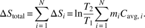
This is an interesting result. It helps us to generalize how the state variable of temperature can be used to measure generated entropy damage for a system that is undergoing some sort of damage related to thermal issues. Note that we do not need to know the temperature of each part; temperature is an intensive thermodynamic variable. It is a roughly uniform indicator for the system. Thus, monitoring temperature change of a large system is one key variable that is a major degradation concern for any thermal-type system.
2.4.5 Example 2.5: Temperature Aging of an Operating System
Prior to a system being subjected to a harsh environment, we make an initial measurement M1+ at ambient temperature T1 and find its operation temperature is T2. Then the system is subjected to an unknown harsh environment. We then return the system to the lab and make a measurement M2+ in the exact same way that M1 was made, where we note it is found to have a different operational temperature T3. Find the aging ratio where
 ,
,
The system has aged by a factor of 1.58. We next need to determine what aging ratio is critical.
2.4.6 Comment on High-Temperature Aging for Operating and Non-Operating Systems
Reliability engineers age products all the time using heat. If this is the type of failure mechanism of concern, then they will often test products by exposing their system to high temperature in an oven. This of course is just one type of reliability test. The product may be operational or non-operational. Often the operational product will add more heat, such as a semiconductor test having a junction temperature rise. Then the true temperature of the semiconductor junction is the junction rise plus the oven temperature. You might ask is there a threshold temperature for aging. The answer is, not really. Temperature aging mechanisms are thermally activated. In a sense, defects are created by surmounting a free energy barrier. Thus, there is a certain probability for a defect to be activated at any given temperature. The most common type of thermally activated aging law is called the Arrhenius Law. The barrier height model is discussed in Chapter 6. However, the Arrhenius Law is found with numerous examples in Chapters 4–10.
2.5 Measuring Randomness due to System Entropy Damage with Mesoscopic Noise Analysis in an Operating System
One might suspect that disorder in the system can introduce some sort of randomness in an operating process of the system. We provide a proof of this in Section 2.6. In this section we assume this randomness is present so we can provide some initial examples first to motivate the reader by demonstrating the importance of noise measurements to assess degradation. Then the reader can first see how it is used to assess aging in operating systems and why it is important. A key example will also be in Section 2.7 on the human heart. First we have to develop some terminology on the measurement process. To start, we define an operating system as follows.
An operating system has a thermodynamic process that generates energy (battery, engine, electric motor…), or has energy passing through the system (transistor, resistor, capacitor, radio, amplifier, human heart, cyclic fatigue…).
Compare this to a non-operating aging system such as metal corrosion, ESD damage, sudden impact failure, internal diffusion, or intermetallic growth. In an operating system there is likely a thermodynamic random variable that is easily accessible, such as current, voltage, blood flow, and so forth.
For example, imagine an electronic signal passing through an electrical system of interest that is becoming increasingly disordered due to aging. We might think the disorder is responsible for a signal to noise problem that is occurring. In fact, we can think of the noise as another continuous extensive variable at the system level (scaling with the size of the system damage). Random processes are sometimes characterized by noise (such as signal to noise). Measuring noise is not initially as obvious as say measuring temperature, which is a well-known thermodynamic state variable. In fact, one does not find noise listed in books on thermodynamics as a state variable. Nevertheless, we can characterize one key state of a system using noise.
Entropy Noise Principle: In an aging system, we suspect that disorder in the system can introduce some sort of randomness in an operating system process leading to system noise increase. We suspect this is a sign of disorder and increasing entropy. Simply put, if entropy damage increases, so should the system noise in the operating process.
This is also true for a non-operating system, except that noise is hard to measure so in that case we will focus on operating systems. For example, an electrical fan blade may become wobbly over time. The increase in how wobbly it is can be thought of as noise, not in the acoustic sense. Its degree of how wobbly it is provides a measure of its increasing “noise level.” Noise is a continuous random variable of some sort.
Measuring randomness due to aging is sometime easy and sometime subtle. For example, a power amplifier may lose power. This is a simple sign of aging and does not require a subtle measurement technique. However, in many cases aging is not so obvious and hard to detect by simple methods. We would like to have a method for refined prognostics to understand what is occurring in the system before gross observation occur, by which time it may be too late to address impending failure. We therefore define what we will term here (for lack of a better phrase):
mesoscopic noise entropy measurement, any measurement method that can be used to observe subtle system-level entropy damage changes that generate noise in the operating system.
To give an indication of what we mean, we note that a macroscopic system contains a large number N of “physical particles,” N > 1020, say. A microscopic system contains a much smaller number N of physical particles, N < 104, say. For the orders of magnitude between these values of N, a new word has been invented. A mesoscopic system is much larger than a microscopic system but much smaller than a macroscopic system. A microcircuit on a chip and a biological cell are two examples of possible mesoscopic systems. Water contained in a bottle is a possible macroscopic system of N molecules of H2O. A single atomic nucleus might be said to form a microscopic system of N bound neutrons and protons. The point is that we are trying to measure details of a system that are not really on the microscopic or the macroscopic level. Therefore, for lack of a better term, we anticipate that such measurements are more on the mesoscopic level. We do not wish to get too caught up in semantics; the reader should just take it as a terminology that we have invented here to refer to the business of making subtle measurements of entropy damage in a system.
One can also use this term for other mesoscopic entropy measurements that are of a different type, for example, scanning electron microscopic (SEM) measurements that are often used to look at subtle damage. This would be another example. However, SEM-type measurements are not of interest in this chapter.
To do this we can treat entropy of a continuous variable using the statistical definition of entropy in thermodynamics employing the concept of differential entropy.
Up until this point we have been using the thermodynamic definition of entropy provided by the experimental definition of entropy. However, we now would like to introduce the statistical definition of entropy. In the simplest form, the statistical definition of entropy is
where kB is the Boltzmann constant, Pi is the probability that the system is in the ith microstate, and the summation is over all possible microstates of the system. The statistical entropy has been shown by Boltzmann to be equivalent to the thermodynamic entropy.
If Pi = 1/N for N different microstates (i = 1,2,…,N) then
which increases as N increases. This helps our notion of entropy. The larger the number of N microstates that can be occupied, the greater is the disorder.
However, since we will be dealing now with randomness variables, in a similar manner we need to work with the statistical definitions of entropy for discrete and continuous variable X. In the same sense entropy is a measure of unpredictability of information content. For a discrete and continuous state variable X, the entropy functions in information theory [3, 4] are written
and for the discrete case extended to the continuum
where X is a discrete random variable in the discrete case and a continuous random variable in the continuous case, and f is the probability density function. The above equation is referred to as the differential entropy [3].
Note that in differential entropy, the variables are usually dimensionless. So if X = voltage, the solutions would be in terms of X = V/Vref, a dimensionless variable.
Here we are concerned with the continuous variable X having probability density function f(x).
2.5.1 Example 2.6: Gaussian Noise Vibration Damage
As an example, consider Gaussian white noise which is one common case of randomness and often reflects many real world situations (note that not all white noise is Gaussian). When we find that a system has Gaussian white noise, the probability density function (PDF) function f(x) is

When this function is inserted into the differential entropy equation, the result is given by [4]
This is a very important finding for system noise degradation analysis, especially for complex systems, as we will see. Such measurements can be argued to be more on the macroscopic level. However, their origins are likely due to collective microstates which we might argue are on the mesoscopic level.
To clarify, for a Gaussian noise system the deferential entropy is only a function of its variance σ2 (independent from the mean μ). This is logical in the sense that, according to the definition of the continuous entropy, it is equal to the expectation value of the log (PDF). For white noise we note that the expectation value of the mean is zero as it fluctuates around zero (see Figure 2.3), but the variance is non-vanishing (see Figure 2.3). Note that the result is also very similar if the noise is lognormally distributed. For a system that is degrading by becoming noisier over time, the entropy damage can be measured in a number of ways where the change in the entropy at two different times t2 and t1 is then [2]


Figure 2.3 Gaussian white noise
2.5.2 Example 2.7: System Vibration Damage Observed with Noise Analysis
Prior to an engine system being subjected to a harsh environment, we make an initial measurement M1+ of the engine vibration (fluctuation) profile which appears to be generating a white noise spectrum in the time domain as is shown in Figure 2.3.
Then the system is subjected to an unknown harsh environment. We again return the system to the lab and make a second measurement M2+ in the exact same way that M1 was made. It is observed that the engine is again generating white noise. The noise measurement spectrum results are
M 1: Engine exhibits a constant power spectral density (PSD) characteristic of 3Grms content in the bandwidth from 10 to 500 Hz.
M 2: Engine exhibits a constant PSD characteristic of 5Grms content in the bandwidth from 10 to 500 Hz.
(Note that standard deviation = Grms for white noise with a mean of zero.) The system noise damage ratio is then:
Note this is the damage aging ratio (see Example 2.5) compared to the damage entropy change given by Equation (2.36). This level of entropy damage ratio indicates a likely issue. It would of course be prudent to have more measurements of other similar engines to assess what the statistical true outliers are.
Interestingly enough, noise engineers are quite used to measuring noise with the variance statistic. That is, one of the most common measurements of noise is called the Allan Variance [5]. This is a very popular way of measuring noise and is in fact very similar to the Gaussian Variance, given by:

where N ≥ 100 generally and τ = sample time. By comparison, the true variance is

We note the Allan Variance commonly used to measure noise is a continuous pair measurement of the population of noise values, while the True Variance is non pair measurement over the entire population. The Allan Variance is often used because it is a general measure of noise and is not necessarily restricted to Gaussian-type noise.
The key results here are that entropy of aging for system noise is dependent on the variance which is also a historical way of measuring noise and is likely a good indicator of the entropy damage of many simple and complex systems.
There are a number of historical options of how noise can be best measured. The author has recently [6, 7] proposed an emerging technology for reliability detection using noise analysis for an operating system. Concepts will be discussed in Section 2.9.
2.6 How System Entropy Damage Leads to Random Processes
Up to this point we have more or less argued that randomness is present in system processes due to an increase in disorder in the system’s materials. We now provide a more formal but simple proof of this.
System Entropy Random Process Postulate: Entropy increase in a system due to aging causes an increase in its disorder which introduces randomness to thermodynamic processes between the system and the environment.
Proof: During an irreversible process we can write the time-dependent change in entropy, where it relates to system entropy change, as:

When the entropy is maximum, aging stops and at that point dSsubsystem(ti) ~ 0, then
That is, any non-damage entropy flow to the environment relates to the entropy damage by the above equation. Furthermore, the total cumulative disorder that has occurred in the material has also had non-damage entropy flow to the environment:

The disorder in the material is then related to the energy flow to the environment. Furthermore, the damage changes to the system’s material is a factor for energy flow. That is, any energy flowing in and out of the system (such as electrical current) can be perturbed by the new disorder in the material. The disorder in energy flow is recognized as a type of randomness and is termed “disordered energy.” It is a random process sometimes referred to as system noise as we have described in this chapter.
Next we need to describe what thermodynamic processes are subject to randomness over time.
System Entropy Damage and Randomness in Thermodynamic State Variables Postulate: Entropy damage in the system likely introduces some measure of randomness in its state variables that are measurable when energy is exchanged between the system and the environment.
Proof: We provide here a sort of obvious proof as it helps to clarify the measurement task at hand. Consider a thermodynamic state variable B(S) that is a function of the entropy S, then to a first-order Maclaurin series expansion we have at time t:
We now consider this at a time later t + τ when disorder has increased due to aging in the system:
Formally, for the thermodynamic variable B we must have
However, we also realize that these two are not totally uncorrelated, that is,
Multiplying B(S(t)) and B(S(t + τ)) together and taking their expectation value, we have:
If we set B(0) = 0 above and B′(0) = K a constant, and ignore the higher-ordered terms, then the measurement task at hand is
This problem reduces to finding what we term as the Noise Entropy Autocorrelation Function:
where RS,S(τ) is the entropy noise autocorrelation function and E indicates that we are taking the expectation value. However, we typically measure RB,B(τ) where it is some thermodynamic state or related function of the entropy.
Here we have assumed that ![]() . But what if
. But what if ![]() ? When work is done on the system and energy is exchanged, we can still have randomness. For example, when a system has been damaged, the material is non-uniform since some measure of disorder occurred. What if it was a resistor for example and we passed current through it? At time t, the current path taken may differ from some later time t + τ as the current path chosen is arbitrarily by the now non-uniform material and is likely a different path in the material to avoid damage sites. The current may even scatter off the damage sites. Here again the current randomness can be measured similarly by the noise autocorrelation function [8], this time for current I where
? When work is done on the system and energy is exchanged, we can still have randomness. For example, when a system has been damaged, the material is non-uniform since some measure of disorder occurred. What if it was a resistor for example and we passed current through it? At time t, the current path taken may differ from some later time t + τ as the current path chosen is arbitrarily by the now non-uniform material and is likely a different path in the material to avoid damage sites. The current may even scatter off the damage sites. Here again the current randomness can be measured similarly by the noise autocorrelation function [8], this time for current I where
If ![]() then we know that it is possible the system damage is creating randomness. In detail, E[I(t), I(t)] is the maximum correlated value so any lower correlated value of the current with its delay τ is likely an indication of system damage. How can we be sure, since it is a subtle measurement? One way is to increase the damage further and make new comparisons. Another way is to take an identical measurement on a similar system that has not experienced damage to have what is termed an experimental control to compare. These concepts are further discussed in detail in Section 2.9.
then we know that it is possible the system damage is creating randomness. In detail, E[I(t), I(t)] is the maximum correlated value so any lower correlated value of the current with its delay τ is likely an indication of system damage. How can we be sure, since it is a subtle measurement? One way is to increase the damage further and make new comparisons. Another way is to take an identical measurement on a similar system that has not experienced damage to have what is termed an experimental control to compare. These concepts are further discussed in detail in Section 2.9.
Formally, there are a number of ways to find the expectation value for the noise autocorrelation function [9]. These are

where in the last integral s1 = S(t), s2 = S(t + τ), and P(s1,s2) = joint PDF of s1 and s2. Note that the autocorrelation function can be normalized by dividing it by its maximum value that occurs when τ = 0, that is:

where
Here E[S(t), S(t)] is the maximum value. We see that any thermodynamic variable that is part of the entropy exchange process between the environment and the system is subjected to randomness stemming from system aging disorder, of which one measurement type is to look at its autocorrelation function.
You might be asking at this point in time, well what does this all mean? In simple terms, an example of an ordered process is people walking out the door of a movie theatre at a rate of one person every 5 s. This is a non random process. Then later we note some randomness; we see that people walk out at an average of 5 s intervals, but occasionally there are people walking out at random times of 1, 2, 3, 4, 6, 7 s intervals. This is initially unpredictable. Prior to randomness being introduced, the autocorrelation was R = 1. Once randomness occurred, R ranged over −1 < R < 1. As more and more randomness is introduced, we expect R to get closer and closer to zero.
Thus, autocorrelation of key state variables is likely a good mesoscopic measure of subtle damage: it is a measure of how random the process has become as degradation increases. If the randomness is stabilized, it is called a stationary random process. However, if randomness in the process is increasing over time, it is a non-stationary random process.
2.6.1 Stationary versus Non-Stationary Entropy Process
Measured data can often be what is termed non-stationary, which indicates that the process varies in time, say with its mean and/or variances that change over time. Although a non-stationary behavior can have trends, these are harder to predict than a stationary process which does not vary in time.
Therefore, non-stationary data are typically unpredictable and hard to model for autocorrelated analysis. In order to receive consistent results, the non-stationary data need to be transformed into stationary data. In contrast to the non-stationary process that has a variable variance and a mean that does not remain near, or return to, a long-run mean over time, the stationary process reverts around a constant long-term mean and has a constant variance independent of time.
Although aging processes are non-stationary, they may vary slowly enough so that in the typical measurement time frame they are stationary. Furthermore, disorder is cumulative which means there is a memory in the process. This means there is a likely trend. The issue is: this is a new way of looking at aging. There are, to this author’s knowledge, few studies on the subject. We describe below one good study on aging of the human heart to help the reader understand the potential importance of noise autocorrelation measurements.
We summarize below what we would anticipate from such a study.
- Entropy randomness mesoscopic measurements.
- If a system has a thermodynamic process that generates energy (battery, engine, electric motor,…) or has energy passing through the system (transistor, resistor, capacitor, radio, amplifier,…), the subtle irreversibilities occurring in the system are likely generating noise in the operating system.
- Non-damage flow exchange that is part of the exchange process related to entropy damage exhibits randomness that we term noise.
- For such subtle system-level damage, we employ the method that we term here as mesoscopic entropy noise measurement analysis to detect subtle changes in the system due to entropy damage. Such damage is not easily detectable by other means.
- This randomness, if measured by one or more thermodynamic state variables, is likely observable from the entropy exchange process with the aid of the autocorrelation function of the state variable.
- Over time, as the system ages, we suspect that the increase in disorder in the system will tend to reduce the autocorrelation result so that the normalized value of RS,S(τ) will approach 0 when the system is in a state of maximum entropy (disorder).
- The aging occurring is likely on a longer time scale than the measurement observation time so that the measurement process can be treated as stationary.
2.7 Example 2.8: Human Heart Rate Noise Degradation
Although noise degradation measurements are difficult to find, one helpful example of noise autocorrelation analysis of an aging system found by the author is in an article by Wu et al. [10] on the human heart.
Here heart rate variability was studied in young, elderly, and congestive heart failure (CHF) patients. Figure 2.4 shows noise limit measurements of heart rate variability. We note that heart rate noise limit variability between young and elderly patients are not dramatically different compared to what is occurring in patients with CHF. Although this is not the same system (i.e., different people), such measurements can be compared using noise analysis described in this section. This is further illustrated in Figure 2.5 showing noise variability in heartbeats of young subjects compared with CHF patients. This is an example of entropy damage comparison in a complex human heart aging system between a good and a failing system observed well prior to catastrophic failure. This reference [10] shows a variation of how our example in Section 2.5 and damage noise entropy mesoscopic measurements in general can be implemented, and would be helpful as a detection method of a system’s thermodynamic degradation state.

Figure 2.4 Noise limit heart rate variability measurements of young, elderly, and CHF patients [10]
Figure 2.5 Noise limit heart rate variability chaos measurements of young and CHF patients [10]
2.8 Entropy Damage Noise Assessment Using Autocorrelation and the Power Spectral Density
In this section we would like to overview more information about the autocorrelation function and detail its Fourier transform to the frequency domain. This is because there is a lot of related work presented in the frequency domain, which is not framed in the category of degradation, which we anticipate is related in many ways. We start by restating the autocorrelation function here for convenience

which was originally described in Equation (2.50). Some properties of the autocorrelation function are:

A graphical representation of the autocorrelation function is shown in Figure 2.6.
Figure 2.6 Graphical representation of the autocorrelation function
The Fourier transform of the autocorrelation function provides what is termed the PSD Spectrum, given by

where f is the frequency. Noise measurements are often easily made with the aid of a noise measurement system that can be purchased. These systems do the math for you, which uncomplicates things. There are some common transforms that are worth noting; these are listed in Table 2.1.
Table 2.1 Common time series transforms
| Time series | Autocorrelation | PSD |
| Pure sine tone | Cosine | Delta functions |
| Gaussian | Gaussian | Gaussian |
| Exponential | Exponential decay | Lorentzian 1/f2 |
| White noise | Decay | Constant |
| Delta function | Delta function | Constant |
For a well-behaved stationary random process, the power spectrum can be obtained by the Fourier transform of the autocorrelation function. This is called the Wiener–Khintchine theorem. Generally, knowledge of one (either R or S) allows the calculation of the other. However, some information can be lost in conversion between say S(ω) to R(τ). As a simple example of a transform and some issues, consider Figure 2.7 that illustrates a Fourier transform of a sine wave with some randomness in the frequency variation. Because of the randomness, this is not a pure sine tone.

Figure 2.7 (a) Sine waves at 10 and 15 Hz with some randomness in frequency; and (b) Fourier transform spectrum. In (b) we cannot transform back without knowledge of which sine tone occurred first
We note that it is difficult to see the variability in frequency in the time series of Figure 2.7a. However, the variability is easily observed from the width of the frequency spectrum in Figure 2.7b. If the signal was a pure sine tone, the Fourier transform would be a delta-function (spike) -like form. Second we note that knowledge of the frequency spectrum will not indicate which wave occurred first; that is clearly indicated in the time series spectrum where the 100 Hz wave occurred first. Therefore, whenever doing this type of analysis, it can be important to look at both the time series and frequency spectrum.
2.8.1 Noise Measurements Rules of Thumb for the PSD and R
Since people are not familiar with noise measurements, we provide some simple rules of thumb to remember.
- As the absolute value of the autocorrelation function decreases to zero, |Rnorm| → 0, noise levels are increasing in the system.
- As the PSD( f ) levels increase, noise is increasing in the system.
- The slope of the autocorrelation function is related to the slope of the PSD spectrum. As the autocorrelation slope increases, the PSD slope decreases. The slope is an indication of the type of system-level noise characteristic detailed in the next section.
2.8.2 Literature Review of Traditional Noise Measurement
There are countless noise measurements in the literature [11]. Here we would like to review well-known noise measurements as we feel it will be helpful in eventually working with degradation problems.
We believe that noise analysis can be crucial in prognostics as we suspect that noise analysis will be a highly important contributing tool. The problem is unfortunately that, at the time of writing of this book, there seems to be little work in the area of noise degradation analysis similar to the human heart study that we have illustrated (i.e., looking at noise as a system ages).
It is clear from our example on the human heart and as we have theoretically shown in Section 2.5 that the noise variance increases with system damage as it is a dependent variable of entropy. This is an indication that the autocorrelation function for system noise is becoming less and less correlated over time for non-stationary processes. As such, we anticipate that the frequency spectrum might have a tendency to higher levels of noise values.
Put another way, as the autocorrelation function becomes less correlated, the PSD spectrum increases. The slope of the PSD curve is an indication of the type of system-level noise observed. Note the slopes of the autocorrelation function and the PSD curve are related. We can clearly see that as the autocorrelation slope decreases (from Figures 2.8b, 2.9b, and 2.10b), the slope of the PSD curve increases (from Figures 2.8c, 2.9c, and 2.10c). Note in Figure 2.8b the slope is hard to see as it decreases quickly near zero time lag. It is possible that the slope may also change in a non-stationary process; we at least expect the noise level to increase. The problem is, as we have mentioned, there is little work in this area to date for non-stationary noise processes.

Figure 2.8 (a) White noise time series; (b) normalized autocorrelation function of white noise; and (c) PSD spectrum of white noise

Figure 2.9 (a) Flicker (pink) 1/f noise; (b) normalized autocorrelation function of 1/f noise; and (c) PSD spectrum of 1/f noise

Figure 2.10 (a) Brown 1/f 2 noise; (b) normalized autocorrelation function of 1/f 2 noise; and (c) PSD spectrum of 1/f 2 noise
Noise is sometimes characterized with color [11]; the three main types in this category are white, pink, and brown noise. Each has a specific type of broadband PSD characteristic. We will first overview these then we will describe some reliability-related type of noise measurements. Each type has an interesting sound that is audible in the human audio frequency range (~20 Hz to 20 kHz) of the spectrum.
Figure 2.8 is a well-known time series that we previously discussed for white noise; see Section 2.5.1 and Figure 2.3. In Figure 2.8b we see the autocorrelation function that starts at 1 (τ = 0) and quickly diminishes, becoming uncorrelated. The PSD spectrum appears to be flat (constant) over the frequency region. However, the variance is non-vanishing. Much work has been done in the area of thermal noise, also known as Johnson noise or Johnson–Nyquist noise, which has a white noise spectrum (see Section 2.9.1).
Figure 2.9 is a well-known phenomenon called 1/f noise, also referred to as pink noise or flicker noise. While many measurements have been carried out and many theories have been proposed, no one theory uniquely describes the physics behind 1/f noise. It is generally not well understood, but is considered by many to be a non-stationary process [11, 12]. From the time series, the autocorrelation function has more correlation over the lag time τ compared to white noise. The fact that it is called 1/f has to do with the slope of the PSD line as shown in Figure 2.9c. In the PSD plot, we see that there is more “power” at low frequencies and appears to diverge at 0.
If we compare figures again, we see that a rapid variation in the time series such as White noise in Figure 2.8 is harder to correlate than a slower variation such as Figure 2.10. In terms of the PSD spectrum, we carefully plotted 1/f and 1/f2 in Figures 2.9 and 2.10c so one can see the relative slope change on the same scale. This is also compared in Figure 2.11. The slope yielding 1/f has been measured over longer periods of lag of just 1 s. There are reports of lags say over 3 weeks with a frequency measured down to 10−6.3 Hz, and the slope continuous to diverge as 1/f with no change in shape [13]. Using geological techniques, the slope of 1/f has been computed down to 10−10 Hz or 1 cycle in 300 years [14].
Figure 2.11 Some key types of white, pink, and brown noise that might be observed from a system
The author anticipates that, if the measurement was taken on semiconductors that had been subjected to parametric aging, the following would hold.
A system undergoing parametric degradation will have its noise level increase. Studies suggest (see Section 2.8.3) for example that

where t is time, subscript V is a system-level state parameter (such as voltage; see Table 1.1), and γ is a power related to the aging mechanism. The system noise would become more uncorrelated yielding a decrease in R for the autocorrelation function and a higher noise level in the PSD spectrum (see Section 2.8.3).
This of course is a statement that the time series changes in aging and, at maximum entropy where failure occurs, we would observe the maximum noise characteristic. There are a number of reasons for this. One key reason is that the material degrades and in effect its geometry is changing due to increasing disorder. For example, a resistor will effectively have less area for current to pass through as the material degrades. In effect the resistor is becoming smaller. We will see in Section 2.8.3 when we look at resistor 1/f type noise characteristics published in the literature that resistors with less area display larger noise levels. Resistors with smaller area handling the same current will have current crowding, which increases noise.
The interesting issue with 1/f noise [11, 12] is that it has been observed in many systems:
- the voltage of currents of vacuum tubes; Zener diodes; and transistors;
- the resistance of carbon resistors; thick-film resistors; carbon microphones; semiconductors; metallic thin-films; and aqueous ionic solutions;
- the frequency of quartz crystal oscillators; average seasonal temperature;
- annual amount of rainfall;
- rate of traffic flow;
- rain drops;
- blood flow;
- and many other phenomena.
Figure 2.10 is another well-known phenomenon called 1/f 2 noise, also referred to as brown (sometimes red) noise, and is a kind of signal-to-noise issue related to Brownian motion. This is sometimes referred to as random walk which is displayed in Figure 2.10a. Here again the slope of the PSD spectrum goes as 1/f 2 (hence the name).
Figure 2.11 compares noise-type slopes on the same graph scale so one can see the relative slopes for a PSD plot.
2.8.3 Literature Review for Resistor Noise
We have mentioned in Section 1.7 that entropy can be produced from resistance. Resistance is a type of friction which increase temperature, creates heat, and often entropy damage. In the absence of friction, the change in entropy is zero. Therefore, it makes sense in our discussion on noise as an entropy indicator that we look at noise in electrical resistors. One excellent study is that of Barry and Errede [15]. These authors found for 1/f noise in carbon resistors that noise measurements on 0.5, 1, and 2 W resistors indicated that the 0.5 W resistors had the largest noise and the 2 W resistors had the least noise. Figure 2.12 illustrates the PSD noise level for carbon resistors as well as the 1/f noise type slopes for these resistors.

Figure 2.12 1/f noise simulations for resistor noise. Note the lower noise for larger resistors (power of 2) and higher noise for smaller resistors (power of 1.5)
We see that resistors with reduced volume or cross-sectional area produce more noise. Other authors have found that 1/f noise intensity for thick-film resistors varies directly with resistance [16, 17]. This is a similar observation as resistor wattage goes as its volume. We can interpret this as an increase in resistance produces higher levels of entropy, increasing disorder, and increasing system-level noise. From an electrical point of view, smaller resistors can produce higher current densities increasing noise. The fact that the noise characteristics are 1/f-type (pink noise) is related to the type of noise phenomenon in the system.
2.9 Noise Detection Measurement System
As an example of how we can use the autocorrelation method on an operating or non-operating system, we can start with the standard electronic system for such measurements. We feel that an active on-board autocorrelation measurement of key telltale parameters can be helpful for prognostics in determining a system’s wellness in real time [6, 7]. Such software methods exist for measurements [7]. Figure 2.13 illustrates a system that can be used for an active measurement process using an electronic multiplier and a delayed signal.

Figure 2.13 Autocorrelation noise measurement detection system
Figure 2.13 shows an initial, say engine vibration, sample at time t, y(t) and with delay τ. This would be a stationary measurement process of the system. The two signals are mixed in the multiplier and averaged. The autocorrelation results can be stored as, say, an engine’s vibration noise sample. Then later we can take another sample at time t2 after the system has been exposed to a stress and compare to see if the noise level has increased. Even though the aging process is non-stationary over time, the actual measurements are stationary as negligible aging occurs during the measurement process. The key difference here is that one is comparing the signals over time. The figure is simplified for a conceptual overview. More sophisticated mixing methods exist [6, 7], as well as prognostic software [7]. The autocorrelated results can of course also be analyzed in the frequency domain with typical PSD magnitude. For random vibration it would have a noise metrics (Grms2/Hz) with Grms spectral content, for voltage noise V2/Hz, etc. Here for engine vibration, one would use accelerometers to generate the y(t) voltage signals (where an accelerometer is a device that converts vibration to voltage), and also look at possible resonance assessment with Q values found from the spectra observations (see Section 4.3.5 for an explanation of resonance and Q effect). Assessment of this type is not limited to engine noise but any type of noise. Noise measurements can be made for electronic circuits, engines, fluid flow, human blood flow (as per the study we presented in Section 2.7), etc.
Such noise measurements can also include amplitude modulation (AM), frequency modulation (FM), or phase modulation noise analysis. For example, a sinusoidal carrier wave can be written
where Amax is its maximum value, ω is the angular frequency, and ϕ is the phase relation. We see that noise modulation can occur to the amplitude, frequency, or phase.
Once noise is captured, one must use engineering/statistical judgment to assess the threshold of the noise issue that can be tolerated before maintenance is warranted.
Statistically, it is easier to judge when maintenance is needed based on a number of such systems. As we gain experience with the type of system we are measuring, the information we obtain is easier to interpret. Therefore, analysis of numerous units when assessed will help determine normality and when maintenance is needed. Typically, a good sample size is likely 30 or greater as the variance of a distribution statistically is known to stabilize for this sample size.
2.9.1 System Noise Temperature
It is not surprising that noise and temperature are related. For example, thermal noise also known as Johnson–Nyquist noise has a white noise spectrum. The noise spectral density in resistors goes directly with temperature and resistance according to the Nyquist theorem, defined as
where R is resistance, T is the temperature, and kB is Boltzmann’s constant [11]. Simply put, as temperature and/or resistance increases, so too will the noise level observed in resistors. Thermal noise is flat in frequency as there is no frequency dependence in the noise spectral density; therefore it is a true example of white noise.
2.9.2 Environmental Noise Due to Pollution
We have asserted that temperature, noise, and failure rate are some good key system thermodynamic state variables. However, depending on how you define the system and the environment, they can also be state variables for the environment. An internal combustion (IC) engine is a system which interacts with the environment causing entropy damage to the environment. This pollution damage and that of other systems, on a global scale, are unfortunately measurable as meteorologists track global climate change. The temperature (global warming) effect is the most widely tracked parameter. However, it might also make sense from what we determined above to look at environmental noise degradation. As our environment ages, we might expect from our above finding that its variance will increase. Some indications of environmental variance change are larger swings in wind, rain, and temperature, causing more frequent and intense violent storms. It might be prudent to focus on such environmental noise issues and not just track global temperature rise [2].
2.9.3 Measuring System Entropy Damage using Failure Rate
So far we have two state variables for measuring aging. Another possible state variable, somewhat atypical but often used by engineers, is the reliability metric called the failure rate λ. We do not think of the failure rate as a thermodynamic state variable. In fact, to any reliability engineer, it is second nature that the failure rate is indeed a key degradation unit of measure that helps to characterize a system in terms of its potential for failure over time. For consistency, we would like to put it in the context of entropy damage to see what we find. For complex systems, the most common distribution used by reliability engineers comes from the exponential probability density function:
The differential entropy can be found easily (see Equation (2.33)) from the negative of the expectation of the natural logarithm of f(x), defined [9]:

where for the exponential distribution the mean E[x] = 1/λ. A way to view this is that the exponential distribution maximizes the differential entropy over all distributions with a given mean and supported on the positive half line (0,∞). This is not a very exciting result, but does provide some physical insight from an entropy point of view on why it is one of the more popular distribution used in reliability for complex systems. So in general, we turned the problem around to the fact that any PDF will maximize the entropy subjected to certain constraints, in this case E[x] = 1/λ. For a normal distribution it is subjected to a mean and sigma over the interval (−∞,∞). In the case of white noise, the results proved helpful in our noise analysis (see Section 2.5).
For the exponential distribution, we note that if the environmental stress changes we can measure the entropy change. In this case, the entropy damage change would be for this system under two different environments:
where the subscripts E1 and E2 are for environments 1 and 2.
2.10 Entropy Maximize Principle: Combined First and Second Law
Typically, entropy change is measured and not absolute values of entropy. We may combine the general first law statement
with the statement of the thermodynamic second law
(for reversible processes, or equilibrium condition). The full statement of the two thermodynamic laws involves only exact differential forms. For a general system the combined statement reads, for a reversible process,
The internal energy U is a function of the entropy and the generalized displacements. During a quasistatic process, the energy change may be decomposed into a term representing the heat flow TdS from the environment into the system plus the work ![]() done by the environment on the system.
done by the environment on the system.
In terms of the entropy function, we have

The entropy maximum principle in terms of aging: Given a set of physical constraints, a system will be in equilibrium with the environment if and only if the total entropy of the system and environment is at a maximum value:
(2.62)
At this point, the system has lost all its useful work, maximum damage has occurred where dS total = 0, and no further aging will occur.
In an irreversible process ![]() , but
, but ![]() for pressure volume work so, for example,
for pressure volume work so, for example, ![]() .
.
The following three examples will help to explain the entropy maximum principle.
2.10.1 Example 2.9: Thermal Equilibrium
Consider a system that can exchange energy with its environment subject to the constraint of overall energy conservation. The total conserved energy is written
where we have dropped the “system” subscript. Under a quasistatic exchange of energy we have
Then, from Equation (2.60) we have
Let’s apply a physical situation to this equation; we can use the conjugate pressure P and volume V thermodynamic work function PdV for YdX. Figure 2.14 displays this example. In the figure we imagine a perfect insulating cylinder so that heat does not escape. It is divided into two sections by a piston which can move without friction. The piston is also a heat conductor. We take the left side to represent the environment and the right side that of the system.

Figure 2.14 Insulating cylinder divided into two sections by a frictionless piston
Since ![]() and, when the volume changes incrementally, we will also have
and, when the volume changes incrementally, we will also have ![]() , we can write
, we can write

and
In order to ensure that the total entropy goes to a maximum, we have positive increments under the exchange of energy in which the system energy change is dU. If the environmental temperature is more than the system temperature, that is, ![]() , then this dictates that
, then this dictates that ![]() and energy flows out of the environment into the system. If the environmental temperature is less than the system temperature, that is,
and energy flows out of the environment into the system. If the environmental temperature is less than the system temperature, that is, ![]() , then this dictates that
, then this dictates that ![]() . The energy then flows out of the system into the environment from the higher-temperature region to the lower-temperature region. A similar argument can be made for the pressure; if P > Penv then dV > 0 and the piston is pushed to the left. If the entropy is at the maximum value, then the first order differential vanishes to yield
. The energy then flows out of the system into the environment from the higher-temperature region to the lower-temperature region. A similar argument can be made for the pressure; if P > Penv then dV > 0 and the piston is pushed to the left. If the entropy is at the maximum value, then the first order differential vanishes to yield

At equilibrium the energy exchange will come to a halt when the environmental temperature is equal to the system temperature, that is, T = Tenv, and P = Penv. This is in accordance with the maximum entropy principle, which occurs when the system and the environment are in equilibrium. This of course is an irreversible process; in thermodynamic terms there is a tendency to maximize the entropy and the pressure and temperature will not seek to go back to the non-equilibrium states. In terms of aging, we might have a transistor that is being cooled by a cold reservoir. Pressure may be related to some sort of mechanical stress. If the transistor fails due to the mechanical stress, the transistor comes to equilibrium with the environment as the pressure is released and the pressure and temperature of the system and environment are equal.
2.10.2 Example 2.10: Equilibrium with Charge Exchange
Shown in Figure 2.15 is a system (capacitor) in contact with an environment (battery).

Figure 2.15 System (capacitor) and environment (battery) circuit
A (possibly) non-linear capacitor is connected to a battery. The capacitor and the battery can exchange charge and energy subject to conservation of total energy and total charge. Then with these constraints we wish to maximize
with the total energy and charge
and
obeying
and
The entropy for the capacitor and battery requires
Then we can write from the combined first and second law equation

or, equivalently,

and
As before when Tenv > T, then dU > 0 energy flows out of the environment into the capacitor system. For E > V, dq > 0 and charge is flowing out of E (battery) into V (capacitor system). For equilibrium when the entropy is maximum, T = Tenv and V = E, so that dStotal = 0. The battery has in a sense degraded its energy in charging the capacitor so that, in the absence of capacitor leakage, no more useful work will occur. Again, the entropy is maximized in the irreversible process. There is no tendency for the charge to flow back into the battery.
2.10.3 Example 2.11: Diffusion Equilibrium
In Chapter 8 for spontaneous diffusion processes we make an analogy to Example 2.10. We find for equilibrium of diffusion into an environment that when the entropy is maximum T = Tenv and μ = μenv. Here T, Tenv, μ, and μenv are system and environmental temperatures and chemical potentials, respectively, prior to diffusion. As well the pressure (P = nRT/V) is the same in system and environmental regions at equilibrium where the system and environment are shown in Figure 8.1. Therefore, atoms or molecules migrate so as to remove differences in chemical potential. Diffusion ceases at equilibrium, when μ = μenv. Diffusion occurs from an area of high chemical potential to low chemical potential. The reader may be interested to work the analogy and compare results to that found in Section 8.1.
2.10.4 Example 2.12: Available Work
Consider a system in a state with initial energy U and entropy S which is not in equilibrium with its neighboring environment. We wish to find the maximum amount of useful work that can be obtained from the system if it can react in any possible way with the environment [4]. Let’s say the system wants to expand to come to equilibrium with the environment and we have a shaft on it that is doing useful work (see Figure 2.16).

Figure 2.16 The system expands against the atmosphere
From the first law we have
The entropy production is
where dSdamage is the increase in entropy damage and δQ/T0 is the entropy outflow. Combining these two equations then the useful shaft work is
Integrating from the initial to final state we have for the actual work

The lost work or the irreversible work associated with the process is
From the second law Sgen > 0 so that the useful work
S gen is positive from Equation (2.80) or zero, so that
is the available work (free energy). Thermodynamics sometimes refers to terms such as exergy or anergy (for an isothermal process) or maximum available work when the final state of the system is reduced to full equilibrium with its environment [4]. In reliability terms this can be a catastrophic failed state.
Consider the situation where W12 has as state 2 the lowest possible energy state so that it is in equilibrium with the environment. This is the maximum availability that gives the maximum useful work. We then take the derivative of this availability A, so with ![]()

which gives

Solving, we get the thermodynamic definitions of temperature and pressure:

We see that these conditions are satisfied when the system has the same temperature and pressure as the environment at the final state. Thus the largest maximum work is possible when the system ends up in equilibrium with the environment. It is also the maximum possible entropy damage SD when the final state of the system has catastrophically failed. Then it is impossible to extract further energy as useful work.
In general, one system can provide more work than another similar system. We can assess the irreversible and actual work as
The efficiency (η) and inefficiency (1–η) of work-producing components can be assessed as
2.11 Thermodynamic Potentials and Energy States
Thermodynamics is an energy approach. We have held off on introducing the thermodynamic potential until this point as we needed to present some examples related to entropy first. We mentioned briefly in Chapter 1 that free energy is roughly opposite to the entropy. As entropy damage increases for the system, the system’s free energy decreases and the system loses its ability to do useful work (see Section 2.5.1). Then instead of focusing on entropy, we can look at the free energy of a system to understand system-level degradation. The thermodynamic potentials are somewhat similar to potential and kinetic energy. When an object is raised to a certain height, it has gained potential energy. When it falls, the potential energy is converted to kinetic energy by the motion. When the object hits the ground, all the potential energy has been converted to kinetic energy. In a similar manner, when we manufacture a device it has a certain potential to do work. This is given by the free energy. When we convert its free energy into useful work, the device’s free energy has been converted into useful work that was done. One way to look at it is that free energy comes down to understanding a system’s available work, which we will show is one of the most important metrics for products in industry. You might ask: do we really need to understand the thermodynamic potentials to do practical physics? We believe it is beneficial to logically understand thermodynamic degradation and these concepts are used in this book.
There are a number of thermodynamic energy states related to the free energy of a system. The free energy is the internal energy minus any energy that is unavailable to perform useful work. The name “free energy” suggests the energy is available or free with the capacity to do work [18]. So these potentials are useful as they are associated with the internal energy capacity to do work. In this section we will use a combined form of the first and second law for the internal energy, written as
to develop a number of other useful relations called the thermodynamic potentials. Note that since we have substituted ![]() , we have assumed a reversible process (see Equation (2.59)) for the moment. The key relations of interest are the Gibbs free energy, Helmholtz free energy, and enthalpy. In the above expression we see that the common natural variables for U are
, we have assumed a reversible process (see Equation (2.59)) for the moment. The key relations of interest are the Gibbs free energy, Helmholtz free energy, and enthalpy. In the above expression we see that the common natural variables for U are ![]() .
.
One of the common interesting properties of a system’s energy state is assessing its lowest equilibrium state. This is true of the internal energy as well. To look at this consider a system that is receiving heat and doing work dU = δQ − PdV (with dN = 0, i.e., no particle exchange), then from the second law
Now consider two conditions, constant entropy and constant volume:
The subscripts mean that V and S are constant, so dV and dS are zero and Equation (2.61) follows. So for constant system entropy, the work is bounded by the internal energy, that is, the work cannot exceed the free energy. The minus sign can be confusing but if one realizes ![]() upon integration, the sign goes away. As well when the entropy (S) and the volume of a closed system are held constant, the internal energy (U) decreases to reach a minimum value which is its lowest equilibrium state. This is a spontaneous process. Another way to think of this is that when the internal energy is at a minimum, any increase would not be spontaneous.
upon integration, the sign goes away. As well when the entropy (S) and the volume of a closed system are held constant, the internal energy (U) decreases to reach a minimum value which is its lowest equilibrium state. This is a spontaneous process. Another way to think of this is that when the internal energy is at a minimum, any increase would not be spontaneous.
2.11.1 The Helmholtz Free Energy
The Helmholtz free energy is the capacity to do mechanical work (useful work). The maximum work is for a reversible process. This is similar to potential energy having the capacity to do work. To develop this potential, we use the chain rule for d(TS) and for PdV work we have:
We insert this expression into the internal energy and arrange the equation as
where we identify the function F = U − TS, known as the Helmholtz free energy. This type of transform is called a Legendre transform; it is a method to change the natural variables. The full expression with particle exchange is
We see the Helmholtz free energy is a function of the independent variables T,V, denoted ![]() .
.
The change in F (ΔF) is also useful in determining the direction of spontaneous change and evaluating the maximum work that can be obtained in a thermodynamic process. To see this we note that for the first law the total work done by a system with heat added to it also includes a decrease in the internal energy dU = δQ – δW and since δQ < TdS (with the inequality for reversible process) then
or
Therefore, when ![]() we have
we have
For an isothermal process (dT = 0), the Helmholtz free energy bounds the maximum useful work that can be performed by a system. As the system degrades, the change in the work capability or lost potential work is due to irreversibilities building up in the system; this change in irreversible work resulting from system degradation causes entropy damage that builds up (or is “stored”) in the system. We note that W can be any kind of work; it can include electrical ore mechanical (pressure–volume) work including stress strain, that is, not just gases.
The equal sign occurs for a quasistatic reversible process, in which case:
Spontaneous degradation: if we had δW = PdV type of work and then decided to hold the volume constant, so that δW = PdV, Equation (2.68) becomes
where
We note that when the system spontaneously degrades (losing its ability to perform useful work), the process requires ![]() . Note this only requires that the change in the Helmholtz free energy has the same temperature and volume in the initial and final states; along the way the temperature and/or volume may go up or down. This does not necessarily account for the total entropy damage Sdamage of the system.
. Note this only requires that the change in the Helmholtz free energy has the same temperature and volume in the initial and final states; along the way the temperature and/or volume may go up or down. This does not necessarily account for the total entropy damage Sdamage of the system.
We can replace the inequality in Equation (2.97) by adding an irreversible term. We find that when we talk about irreversible processes in Section 2.11.5, for dT = 0 the actual work change is
This is an important result as it connects the concept of work, free energy, and entropy damage.
2.11.2 The Enthalpy Energy State
Enthalpy is the capacity to do non-mechanical work plus the capacity to release heat. It is often used in chemical processes. To develop enthalpy, we write PdV using the chain rule
Then we substitute this into the internal energy and manipulate it as
H is called the enthalpy and we can write it as ![]() . The full expression for the enthalpy with particle exchange is
. The full expression for the enthalpy with particle exchange is
We see that enthalpy is a function of the natural variables (S, P), that is, ![]() . At constant pressure
. At constant pressure ![]() (isobaric) and without particle exchange
(isobaric) and without particle exchange ![]() ; then
; then ![]() . This says the enthalpy tells one how much heat is absorbed or released by a system. If for example we have an exothermic reaction where heat flows out of the system to the surroundings, the entropy of the surroundings increases so
. This says the enthalpy tells one how much heat is absorbed or released by a system. If for example we have an exothermic reaction where heat flows out of the system to the surroundings, the entropy of the surroundings increases so ![]() . It is common knowledge that a chemical reaction will be spontaneous when the Gibbs free energy (described in the following section) is negative. We mention this because the Gibbs free energy G can be given in terms of the enthalpy
. It is common knowledge that a chemical reaction will be spontaneous when the Gibbs free energy (described in the following section) is negative. We mention this because the Gibbs free energy G can be given in terms of the enthalpy ![]() which helps explain ΔH. So from this relation, we note that if ΔH is negative and the entropy is increasing than
which helps explain ΔH. So from this relation, we note that if ΔH is negative and the entropy is increasing than ![]() and the reaction will proceed.
and the reaction will proceed.
2.11.3 The Gibbs Free Energy
The Gibbs free energy is the capacity to do non-mechanical work. The maximum work is for a reversible process. This is similar to potential energy having the capacity to do work. To develop the Gibbs free energy we again use the chain rule for d(PV). This time we start by inserting it into the Helmholtz free energy for convenience, obtaining
which can be arranged as
Here we identify the function ![]() , which is called the Gibbs free energy. We see the Gibbs free energy is a function of the independent variables
, which is called the Gibbs free energy. We see the Gibbs free energy is a function of the independent variables ![]() . Some other relations of interest include
. Some other relations of interest include ![]() or writing it in terms of the enthalpy
or writing it in terms of the enthalpy ![]() .
.
We have that ![]() , writing
, writing ![]() , where other work refers to non P–V mechanical work such as electrical work. Then at constant temperature and pressure
, where other work refers to non P–V mechanical work such as electrical work. Then at constant temperature and pressure
But by definition, dH = dU + PdV so that
For an isothermal process at constant pressure, the Gibbs free energy bounds the maximum amount of useful work that can be performed by a system, that is:
As the system degrades, the change in the work capability or lost potential work is due to irreversibilities building up in the system; this change in irreversible work resulting from system degradation causes entropy damage that is built-up (or “stored”) in the system.
In a similar manner to Equation (2.100), we can replace the inequality above by adding the irreversible term
If a system is in contact with a heat reservoir meaning constant temperature, and if the pressure is constant, then the change in the Gibbs free energy is
The change in the entropy of the system and the reservoir is
where Q = −QR. Since ΔS must increase in any process then the Gibbs free energy change must decrease having a negative change in value, ΔG ≤ 0, when the temperature and pressure are constant in a degradation process.
The Gibbs free energy is a popular function to use when there is particle exchange with the surroundings. In this case, the internal energy is also a function of N so U = U(S,V,N).
From Table 1.1, inserting chemical work, we can write
From the above Legendre transform, following the same methods (Equation (2.92)),
Most commonly one considers reactions at constant P and T, so the Gibbs free energy is the most useful potential in studies of chemical reactions as it simplifies to
2.11.4 Summary of Common Thermodynamic State Energies
From these definitions we can say that ΔU is the energy added to the system, ΔF is the total work done on it, ΔG is the non-mechanical work done on it, and ΔH is the sum of non-mechanical work done on the system and the heat given to it. When we are concerned with the conjugate variables (S, T) and (P, V), we note there are only four possible pairs of independent variables. The only time that we would need to change variables is when we use other types of thermodynamic work besides (P, V).
Table 2.2 summarizes the four types of energies.
Table 2.2 Four common thermodynamic potential and energy states
| Name | Formula | Properties | Derivatives |
| Internal energy U(S, V) |
|
First law: ΔU = Q – W |

|
| Helmholtz free energy F(T, V) |
|
ΔF ≤ 0; T, V constant |

|
|
Enthalpy H(S, P) |
|
Isobaric process: ΔH = Q |

|
| Gibbs free energy G(T, P) |
Also of interest: |
ΔG ≤ 0; T, P constant when G = G(T, P, N) and |

|
2.11.5 Example 2.13: Work, Entropy Damage, and Free Energy Change
Let’s consider an irreversible process to illustrate some of the ideas in this section with respect to system entropy damage, free energy, and internal energy.
We wish to see how much work can be extracted from a system even during an irreversible process. One way to think of this is to take in heat and see how much work the system can provide. This is illustrated in Figure 2.17. By conservation of energy from the first law for Figure 2.17 we have
Figure 2.17 Mechanical work done on a system
Associated with irreversible process will be damage that is occurring in the system (or device). Some of the heat goes into damage (say due to friction) and some into work. Keeping tabs on the system entropy we have
Solving for δQ we have
and by rearranging terms in Equation (2.115) and inserting the above we obtain
For the moment let’s consider a reversible process so that dSdamage = 0. This gives us the maximum work for a reversible process
If dT = 0 for an isothermal process we can write this as
Therefore, the change in the Helmholtz free energy is defined as the maximum amount of useful work that can be obtained from a system. The work found from the integral going from a system state 1 to 2 in a reversible way is

Now what about the irreversible process? We need to somehow account for what happens to the system’s free energy. When in state 1 we know that its free energy is F1. In that state it had a certain capacity to do work which was bounded by the free energy F1, so the work capability was ![]() .
.
The path-dependent work causes resistance or friction and the actual work in going to state 2 was really
So now state 2 has a different free energy then state 1 due to the entropy damage. Note that we have dropped the minus sign for the work as it is understood we seek the useful work that a system does.
Now if we continued to do work to a final equilibrium state FN in an incremental way we would get to the minimum value of the free energy Fmin, but over the same path we would have
We can visualize this incremental process with the aid of the Figure 2.18 for a system that has undergone an irreversible process and incurred entropy damage between state 1 and state 2. There is no way to reverse the entropy damage. According to the second law, dS > 0 for the irreversible process and entropy increase means the system disorder has increased. If state 2 happens to be its lowest energy state then no further work can occur; the system has likely failed catastrophically so entropy damage stops, ![]() , and the change in the free energy goes to zero
, and the change in the free energy goes to zero ![]() .
.

Figure 2.18 Loss of available work due to increase in entropy damage
When we talk about dT = 0 it is more appropriate to say that only the initial and final states need to have the same temperature. In between they can fluctuate. We can write the incremental change in the work as
or
This is consistent with Equation (2.87). The efficiency of the work process is then
At this point we can start modeling the actual work and the irreversible work. For example we might write
Since the reversible work (the maximum work) can be treated as fixed, the rate of actual work is some function of the rate of the irreversible work over the work path
These last equations seem harmless enough but they are important results. These work functions are independent of whether we talk about a chemical process where we are using the Gibbs free energy, an electric, or a mechanical process using the Helmholtz free energy. If you are a pragmatic person, the last few equations give you a great bottom line for thermodynamics because no matter how complicated thermodynamics is, a big part of it is undeniably all about work.
For this problem the general expression for power is:
Now the work left that is available in state 2 can be more time related than power loss related. That is, the system has lost some strength from the irreversible process U12; however, it may very well be able to keep on performing its intended function until its free energy is all used up. We provided an example in Section 2.1 on Miner’s rule (see also Chapter 4) that is commonly used to interpret the work left in terms of cycles of remaining (time) and not power or strength loss.
We also note that the entropy damage is path dependent on how the work was performed. As we mentioned in Chapter 1 we are staying away from using too many confusing symbols but, in reality, we should be mindful about the path dependence related to the work path for which we should be writing dSdamage and dSnon-damage as δSdamage and δSnon-damage.
2.11.6 Example 2.14: System in Contact with a Reservoir
Consider a special case of a system that is in contact with a heat reservoir, as shown in Figure 2.19. If there is no mechanical work PdV = 0 with constant volume ΔU = ΔQ. Then

Figure 2.19 A simple system in contact with a heat reservoir
Then the total entropy change is
where ![]() .
.
Note that the total entropy ![]() so we can also write
so we can also write
The Helmholtz free energy never increases in a spontaneous process with fixed temperature and volume in a system in contact with a heat reservoir. We see this causes the entropy to increase since ![]() . To emphasize this, as the system’s entropy increases, its free energy will have a tendency to decrease if it can. Figure 2.20 shows the possible spontaneous decay of a system’s free energy over time to its final descent to its equilibrium state and the corresponding total entropy increase.
. To emphasize this, as the system’s entropy increases, its free energy will have a tendency to decrease if it can. Figure 2.20 shows the possible spontaneous decay of a system’s free energy over time to its final descent to its equilibrium state and the corresponding total entropy increase.

Figure 2.20 A system’s free energy decrease over time and the corresponding total entropy increase
We note that we have sketched the free energy which decays in a non-linear way. This is not atypical of systems.
2.11.6.1 Full Expression for Potential with Entropy Damage
General work-related processes and exchanges with the system’s internal energy require different relationships. For example, consider the full assessment without any conditions on the Helmholtz free energy and temperature where particles can flow in or out of the system; then the general change in the work is
where Ni is the number of particles or moles in the system of species i. Note in Section 2.11.1 we used conditions dT = dN = 0. One needs to account for sign changes depending on the particular conditions as well.
If we have a situation of constant temperature and pressure (dT = dP = 0) we will obtain the similar results in terms of the Gibbs free energy
The general assessment without any conditions on the Gibbs free energy is
If we have a situation of constant pressure and entropy flow (dT = dS = 0) we will obtain similar results in terms of the enthalpy:
The general assessment without any conditions on the enthalpy is
Lastly, the internal energy is
References
- [1] Miner, M.A. (1945) Cumulative damage in fatigue. Journal of Applied Mechanics, 12, A159–A164.
- [2] Feinberg, A. (2014) Thermodynamic damage within physics of degradation, in The Physics of Degradation in Engineered Materials and Devices (ed J. Swingler), Momentum Press, New York.
- [3] Shannon, C.E. (1948) A mathematical theory of communication. Bell System Technical Journal, 27 (3), 379–423.
- [4] Hazewinkel, M. (ed) (2001) Differential entropy, in Encyclopedia of Mathematics, Springer, New York.
- [5] Allan, D. (1966) Statistics of atomic frequency standards. Proceedings of IEEE, 54 (2), 221–230.
- [6] Feinberg A. Thermodynamic damage measurements of an operating system. Proceedings of the 2015 Annual Reliability and Maintainability Symposium (RAMS), January 26–29, 2015, Palm Harbor, FL. IEEE Xplore.
- [7] Feinberg A. Active autocorrelation noise detection degradation spectroscopy library measurement device. US Patent 62/284,056, Sept 21, 2015. (For prognostic noise measurement software tools, interested readers should contact the author through his website http://www.dfrsoft.com.)
- [8] Buckingham, M.J. (1985) Noise in Electronic Devices and Systems, John Wiley & Sons, Inc, New York.
- [9] Dunn, P.F. (2005) Measurement and Data Analysis for Engineering and Science, McGraw–Hill, New York.
- [10] Wu, G.Q., Arzeno, N.M., Shen, L.L., Tang, D.K., Zheng, D.A., Zhao, N.Q., Eckberg, D.L. Chaotic signatures of heart rate variability and its power spectrum in health, aging and heart failure. PLoS One,2009, 4 (2), e4323.
- [11] Musha, T., Sato, S. and Yamamot, M. (eds) (1992) Noise in Physical Systems and 1/f Fluctuations, IOS Press, Amsterdam.
- [12] Keshner, M.S. (1982) 1/f noise. Proceedings of the IEEE, 70 (3), 212–218.
- [13] Caloyannides, M.A. (1974) Microcycle spectral estimates of l/f noise in semiconductors. Journal of Applied Physics, 45 (1), 307–316.
- [14] Mandelbrot, B.B. and Wallis, J.R. (1969) Some long-run properties of geophysical records. Water Resources Research, 5 (2), 321–340.
- [15] Barry, P., Errede, S. Measurement of 1/f noise in carbon composition and thick film resistors. Senior thesis, Phys 499, Fall 2014, University of Illinois.
- [16] de Jeu, W.H., Geuskens, R.W.J. and Pike, G.E. (1981) Conduction mechanisms and 1/f noise in thick-film resistors with Pb3Rh7015 and PbQRU207. Journal of Applied Physics, 52, 4128.
- [17] Wolf, M., Muller, F. and Hemschik, H. (1985) Active Passive. Electronic Components, 12, 59.
- [18] Morse, P.M. (1969) Thermal Physics, Benjamin/Cummings Publishing, New York.