Chapter 4
Semi-Empirical Tire Models
Chapter Outline
4.3. The Magic Formula Tire Model
Longitudinal Force (Pure Longitudinal Slip, α =0)
Lateral Force (Pure Side Slip, κ = 0)
Aligning Torque (Pure Side Slip, κ = 0)
Longitudinal Force (Combined Slip)
Normal Load (see also Eqns (7.48) and (9.217))
4.3.5. Overturning Couple (also see Section )
Rolling Resistance Moment (see Eqns (9.236, 9.230, 9.231))
Aligning Torque (combined slip)
4.3.3. Extension of the Model for Turn Slip
Note on the Aligning Torque at Large Camber
4.3.6. Comparison with Experimental Data for a Car, a Truck, and a Motorcycle Tire
4.1 Introduction
In the preceding chapter the theory of the tire force and moment generating properties have been dealt with based on physical tire models. The present chapter treats models that have been specifically designed to represent the tire as a vehicle component in a vehicle simulation environment. The modeling approach is termed ‘semi-empirical’ because the models are based on measured data but may contain structures that find their origin in physical models like those treated in the preceding chapter. The mathematical descriptions are restricted to steady-state situations. The non-steady-state behavior will be discussed in subsequent chapters.
In the past, several types of mathematical functions have been used to describe the cornering force characteristic. Exponential, arctangent, parabolic (up to its maximum), and hyperbolic tangent functions (difference of two) have been tried with more and less success. Often, only very crude approximations could be achieved. To improve the accuracy, tables of measured data points have been used together with interpolation schemes. Also, higher-order polynomials were popular but proved not to be always suitable in terms of accuracy and the very large deviations that occur outside the ranges of slip covered by the original measurement data used in the fitting process. Mathematical representations of longitudinal force and aligning torque came later, and only relatively recently the combined slip condition was included in the empirical description. The longitudinal slip ratio was introduced as an input variable instead of the braking or driving force which was common practice in the early days of vehicle dynamics analysis. This latter method, however, is still in use for certain applications.
In the following sections of this chapter, first, a relatively simple approach will be discussed that is based on the similarity concept and after that, in the remainder of the chapter, a detailed description will be given of the Magic Formula tire model. The two model approaches belong to the second and first categories of Figure 2.11, respectively.
4.2 The Similarity Method
The method to be discussed in this section is based on the observation that the pure slip curves remain approximately similar in shape when the tire runs at conditions that are different from the reference condition. The reference condition is defined here as the state where the tire runs at its rated (nominal) load (Fzo), at camber equal to zero (γ = 0), at either free rolling (κ = 0) or at side slip equal to zero (α = 0) and on a given road surface (μo). A similar shape means that the characteristic that belongs to the reference condition is regained by vertical and horizontal multiplications and shifting of the curve. The similarity method is based on the normalization theory of Fiala (1954) and has been introduced by Pacejka (1958), also cf. Radt and Pacejka (1963) and Pacejka (1971, 1981). A demonstration that, in practice, similarity indeed approximately occurs is given by Radt and Milliken (1983), also see Milliken and Milliken (1995). Figures 4.1 and 4.2 present the results when the force and moment as well as the slip angle have been normalized, resulting in the nondimensional quantities shown along the axes. The raw data have been processed to make the characteristics pass through the origin of the graph. The curve results from a Magic Formula fit. The parameters B′, C′, D′, and E′ for the nondimensional side force (subscript y) and for the nondimensional moment (subscript z) have been used in the nondimensional version of the Magic Formula given in Eqn (1.6) and similar for the moment. Further on, the formula will be introduced again, Eqns (4.6, 4.10).
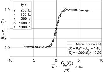
FIGURE 4.1 Result of Radt’s nondimensionalization of tire characteristics showing that the tire side force characteristics measured at different loads reduce to virtually the same curve when the force and the slip angle are normalized as indicated.
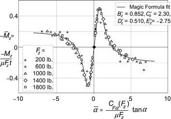
FIGURE 4.2 Result of Radt’s nondimensionalization of the tire aligning torque characteristic after normalizing the moment and the slip angle as indicated; t represents the pneumatic trail at vanishing slip angle.
The resulting model is, through its simplicity, relatively fast. It is capable to represent pure slip conditions rather well including the influence of a camber angle. The description of the situation at combined lateral and longitudinal slip is qualitatively satisfactory. Quantitatively, however, deviations may occur at higher levels of the combined two slip values.
4.2.1 Pure Slip Conditions
The functions representing the reference curves which are found at pure slip conditions are designated with the subscript o. We have, for instance, the reference function Fy = Fyo(α) that represents the side force vs slip angle relationship at nominal load Fzo, with longitudinal slip and camber equal to zero and the friction level represented by μo. We may now try to change the condition to a situation at a different wheel load Fz. Two basic changes will occur with the characteristic: (1) a change in level of the curve where saturation of the side force takes place (peak level) and (2) a change in slope at vanishing side slip (α = 0). The first modification can be created by multiplying the characteristic both in vertical and horizontal direction with the ratio Fz/Fzo. The horizontal multiplication is needed to not disturb the original slope. We obtain, for the new function,
![]() (4.1)
(4.1)
with the equivalent slip angle:
![]() (4.2)
(4.2)
Because, obviously, the derivative of Fyo with respect to its argument αeq at αeq = 0 is equal to the original cornering stiffness CFαo, we find, for the derivative of Fy with respect to α the same value for the slope at α = 0,
![]() (4.3)
(4.3)
which proves that the slope at the origin of the characteristic is not affected by the successive multiplications. The second step in the manipulation of the original curve is the adaptation of the slope. This is accomplished by a horizontal multiplication of the newly obtained characteristic. This is done by multiplying the argument with the ratio of the new and the original cornering stiffness. Consequently, the new argument reads
![]() (4.4)
(4.4)
Together with Eqn (4.1) we have the new formulation for the side force vs slip angle relationship at the new load Fz. In Figure 4.3 the two steps taken to obtain the new curve have been illustrated. Here, the nominal load Fzo = 3000 N and the new load Fz = 1500 N.
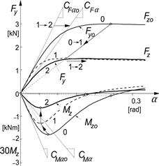
FIGURE 4.3 Using the similarity method to adapt Fy and Mz curves to new load level.
In the same figure the characteristic of the aligning torque has been adapted to the new condition. For this, we use the knowledge gained when working with the brush model (cf. Figure 3.4). More specifically, we will obey the rule that according to the theory, obviously, the point where the Mz curve reaches the α axis lies below the peak of the Fy curve. In Figure 3.4 this occurs at tan α = 1/θy. This requirement means that the same equivalent slip angle (4.4) must be used as for the argument of the Fy function (4.1). In addition, we will use information on the new value of the aligning stiffness CMα. The reference curve for Mz0 that is used is more realistic than the theoretical curve of Figure 3.4. Typically, the moment changes its sign in the larger slip angle range where Fy reaches its peak.
With the same equivalent slip angle and the new aligning stiffness, we obtain the expression for the new value of the aligning torque according to the similarity concept:
![]() (4.5)
(4.5)
The first and third factors being the inverse of the multiplication factor used in (4.4) are needed to maintain the original slope. The second factor multiplies the intermediate Mz curve (1 in Figure 4.3) in vertical direction to adapt the slope to its new value (2) while not disturbing the α scale. It may be noted that the combined second and third factor equals the ratio of the new and the original values of the pneumatic trail t/to.
For the calculations connected with Figure 4.3, the reference characteristics for Fyo, Mzo, and CFα have been described by means of the Magic Formula type functions (cf. Eqn (1.6)). For this occasion, the aligning stiffness is modeled as the product of a certain fraction of the contact length 2a and the cornering stiffness. The resulting characteristics for these four quantities as shown in Figures 4.3 and 4.4 are realistic. The following formulas have been used:
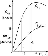
FIGURE 4.4 Cornering and aligning stiffness vs wheel load.
Side force at nominal load Fzo
![]() (4.6)
(4.6)
with stiffness factor
![]() (4.7)
(4.7)
peak factor for the side force which in general is different from the one for the longitudinal force; consequently we introduce μyo besides μxo:
![]() (4.8)
(4.8)
and cornering stiffness as function of wheel load Fz:
![]() (4.9)
(4.9)
Aligning torque at nominal wheel load:
![]() (4.10)
(4.10)
with stiffness factor
![]() (4.11)
(4.11)
peak factor (ao representing half the contact length at nominal load)
![]() (4.12)
(4.12)
and aligning stiffness as function of wheel load Fz
![]() (4.13)
(4.13)
where apparently the pneumatic trail t = c4 a. Half the contact length a is assumed to be proportional with the square root of the wheel load:
![]() (4.14)
(4.14)
The resulting approximation of the pneumatic trail turns out to be quite adequate and might be considered to be used in the set of Magic Formula tire model Eqn (4.E42) to be dealt with later on.
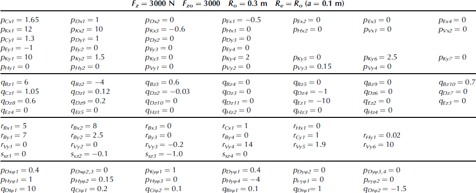
The values of parameters used for the calculations to be conducted have been listed in Table 4.1.
TABLE 4.1 Parameter Values used in Section 4.2
The next two items we will deal with are a change in friction coefficient from μyo to μy and the introduction of a camber angle γ. The first change can be handled by multiplying the curves in radial direction with factor μy/μyo. Together with the change in load, we find
![]() (4.15)
(4.15)
with
![]() (4.16)
(4.16)
The friction coefficient may be assumed to depend on the slip velocity Vs. To model the situation on wet roads, a decaying function μ(Vs) may be employed, cf. e.g., Eqn (4.E23).
When considering the computed characteristics of Figure 3.35c (2nd row) for small camber angles, a horizontal shift of the Fy curve may give a reasonable result. Then, the peak side force remains unchanged which is a reasonable assumption but not always supported by experimental evidence (where often, but not always, a slight increase in maximum side force is manifested) or by computations with a physical model with constant friction and finite contact width which show a slight decrease. For small angles, the camber thrust is approximated by the product of the camber stiffness and the camber angle: Fyγ = CFγγ. Consequently, the α shift should amount to
![]() (4.17)
(4.17)
so that
![]() (4.18)
(4.18)
which gives rise to αeq (4.16) with α replaced by ![]() .
.
For the representation of the aligning moment at the new conditions, the situation is more complex. We observe from Figure 3.35c that for not too large slip angles, the original curve Mzo tends to shift both sideways and upward. If the same equivalent slip angle and thus the same horizontal shift (4.17) as for the force is employed, the moment would become zero where also the force curve crosses the α-axis. A moment equal to −CMα SHy would arise at α = 0. However, the moment should become equal to CMγγ, with a positive camber moment stiffness CMγ. This implies that an additional vertical shift required is equal to
![]() (4.19)
(4.19)
This additional moment corresponds to the so-called residual torque Mzr, which is the moment that remains when the side force becomes equal to zero. For larger values of the slip angle, the additional moment should tend to zero as can be observed in Figure 3.35c. This may be easily accomplished by dividing (4.19) by a term like 1 + c7 α2, cf. Eqn (4.26).
The dependencies of the camber stiffnesses on the vertical load may be assumed linear. We have
![]() (4.20a)
(4.20a)
where b denotes half the (assumedly constant) width of the contact patch, re the effective rolling radius, and CFκ the longitudinal slip stiffness which is considered to be linearly increasing with load:
![]() (4.20b)
(4.20b)
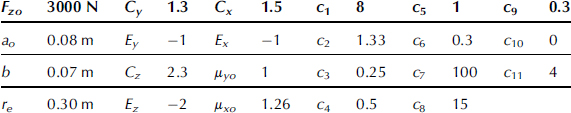
In Figure 4.5, the different steps leading to the condition with a (small) camber angle have been demonstrated. First, the original curve (0) is moved to the left over a distance equal to the horizontal shift (4.17) yielding the intermediate curve (1). Then the residual torque is added: vertical shift (4.19), possibly made a function of slip angle by multiplying the shift with a decaying weighting function as suggested above. The load Fz and the friction coefficient μy have been kept equal to their reference values: 3000 N and 1, respectively.
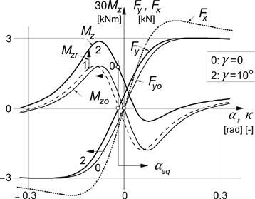
FIGURE 4.5 Introduction of a camber angle in the side force and the aligning torque vs side slip characteristics according to the similarity method. The longitudinal force vs longitudinal slip characteristic (not affected by camber). (Fz = Fzo = 3000 N, μy = μyo = 1, μx = μxo = 1.26).
The longitudinal force at pure longitudinal slip may be modeled in the same way as we did for the side force. Equations similar to (4.6– 4.8) hold for the reference function. An influence of camber on the longitudinal force, however, is assumed not to occur. In the same Figure 4.5, the characteristic for Fx vs κ has been drawn. The values of the relevant additional parameters for the longitudinal force and the moment have been listed in Table 4.1.
We finally have the following similarity formulas for pure slip conditions (either at longitudinal or at lateral slip) for the longitudinal force:
![]() (4.21)
(4.21)
with the equivalent longitudinal slip
![]() (4.22)
(4.22)
and, for the side force,
![]() (4.23)
(4.23)
with the equivalent slip angle, containing the horizontal shift (4.17):
![]() (4.24)
(4.24)
![]() (4.25)
(4.25)
with the residual torque corresponding to the vertical shift (4.19) provided with the reduction factor:
![]() (4.26)
(4.26)
4.2.2 Combined Slip Conditions
We will now address the problem of describing the situation at combined slip. The analysis of the brush model has given considerable insight into the mechanisms that play a role and we will use the theoretical slip quantities σx,y (Eqn 3.34 or 3.32) and the magnitude σ(3.40) and we will adopt the concept similar to that of assessing the components of the resulting horizontal force according to (3.49) and consider the pneumatic trail t as in (3.50) and include explicit contributions of Fx to the moment as indicated in (3.51). We have, for the theoretical slip quantities with the α shift due to camber included,
![]() (4.27a)
(4.27a)
![]() (4.27b)
(4.27b)
and
![]() (4.28)
(4.28)
with
![]() (4.29)
(4.29)
In the ensuing theory, we will make use of the theoretical slip quantities ![]() and
and ![]() (4.27a, b). By using these quantities, the slope in the constant α curves in the Fy vs Fx diagram at Fx = 0 does show up, like for the brush model in Figure 3.13. It should be noted, however, that experience shows that the use of practical slip quantities
(4.27a, b). By using these quantities, the slope in the constant α curves in the Fy vs Fx diagram at Fx = 0 does show up, like for the brush model in Figure 3.13. It should be noted, however, that experience shows that the use of practical slip quantities ![]() and
and ![]() (that is: κ and tan
(that is: κ and tan![]() which may be obtained again by omitting the denominators in (4.27a, b)) may already give very good results as will be indicated later on in Figure 4.8. Note that when approaching wheel lock
which may be obtained again by omitting the denominators in (4.27a, b)) may already give very good results as will be indicated later on in Figure 4.8. Note that when approaching wheel lock ![]() . This calls for an artificial limitation by adding a small positive quantity to the denominator of (4.27a).
. This calls for an artificial limitation by adding a small positive quantity to the denominator of (4.27a).
Because we are dealing with an in general nonisotropic tire, we have pure longitudinal and lateral slip characteristics that are not identical (cf. Figure 4.5). Still, we will take the lateral and longitudinal components but then of the respective pure slip characteristics Fyo and Fxo. If we want to use the theoretical slip quantities σ, we must have available the pure slip characteristics with σx and σy as abscissa. This can be accomplished by fitting the original data after having computed the values of σx for each value of κ by using (4.27a) and similarly for transforming α into tan α and denoting the resulting functions: Fxo(σx), Fyo(σy), and Mzo(σy). Or, simpler, by replacing in the already available pure slip force and moment functions, expressed in terms of the practical slip quantities, the argument α (in radians) by tan α (probably acceptable approximation) and κ by the expression given below (derived from Eqn (4.27a)),
![]() (4.30)
(4.30)
which would be successful if the Fx characteristic had been fitted for the whole range of positive (driving) and negative (braking) values of κ. Otherwise if only the braking side is available (κ and σx < 0) and the driving side is modeled as the mirror image of the braking side, one might better take
![]() (4.30a)
(4.30a)
If the thus obtained function of Fx is plotted vs σx, the resulting curve becomes symmetric. However, if then the abscissa is converted into κ by using (4.30), the resulting Fx(κ) curve turns out to become asymmetric with the braking side identical to the characteristic we started out with. This asymmetry was already found to occur with the brush model discussed in Chapter 3.
In the combined slip model that we employ, the longitudinal and lateral force components are obtained according to an adapted Eqn (3.49) where for the side force F(σ) is replaced by Fyo(σ) and, for the fore-and-aft force, F(σ) is replaced by Fxo(σ). Figure 4.6 illustrates the procedure. The figure shows how the force vector arises from the individual pure slip characteristics. At small slip, due to slip stiffness differences, the vector does not run opposite with respect to the slip speed vector Vs. At wheel lock, however, the force vector does run opposite with respect to the slip speed vector because it is assumed here that the levels of the individual characteristics (asymptotes) are the same for the slip approaching infinity (in the Magic Formula, we should have μyo sin(½π Cy) = μxo sin(½π Cx)).
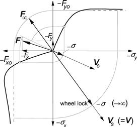
FIGURE 4.6 Construction of the resulting combined slip force from the pure slip characteristics according to Eqn (4.31) (with camber not considered).
Next, we should realize that through (4.18) camber has been accounted for and that, as a consequence, σy is to be replaced by ![]() defined by Eqn (4.27b). The resulting force and moment functions are denoted by Fxo(σx), Fyo
defined by Eqn (4.27b). The resulting force and moment functions are denoted by Fxo(σx), Fyo![]() , and Mzo
, and Mzo![]() . The components now become, with
. The components now become, with ![]() denoting the magnitude of the theoretical slip vector (4.28),
denoting the magnitude of the theoretical slip vector (4.28),
![]() (4.31)
(4.31)
At large slip, the model apparently fails to properly account for the contribution of the camber angle. At wheel lock, one would expect the side force to become zero at vanishing slip angle. This will not exactly be the case in the model due to the equivalent theoretical side slip defined according to Eqn (4.27b) with ![]() given by (4.18).
given by (4.18).
For the aligning torque, we may define
![]() (4.32)
(4.32)
with the first term directly attributable to the side force. This term can be written as
![]() (4.33)
(4.33)
By considering (4.31), it turns out that (4.33) becomes
![]() (4.34)
(4.34)
The last three terms of Eqn (4.32) result from the moment exerted by the longitudinal force because of the moment arm that arises through the side force-induced deflection, a possibly initial offset of the line of action and the sideways rolling of the tire cross section due to camber. For the sake of simplicity, these effects are assumed not to be influenced by the wheel load.
With the similarity expressions for the pure slip forces Fx,yo and moment ![]() , we finally obtain the following formulas for combined slip conditions. For the longitudinal force
, we finally obtain the following formulas for combined slip conditions. For the longitudinal force
![]() (4.35)
(4.35)
![]() (4.36)
(4.36)
and, for the side force,
![]() (4.37)
(4.37)
with the equivalent slip
![]() (4.38)
(4.38)
and, for the aligning torque,
 (4.39)
with the residual torque
![]() (4.40)
(4.40)
On behalf of example calculations, the three additional nondimensional parameters c9, c10, and c11 have been given values listed in Table 4.1.
For the case of a load different from the reference value and the presence of a camber angle, the combined slip characteristics for the tire side force and for the aligning torque have been assessed by using the above equations. The resulting diagrams with slip angle α used as parameter have been presented in Figures 4.7a and b. Due to the use of the theoretical slip quantities (4.27a, 4.27b) in the derivation, we find that the curves of Fy vs Fx show the slight slope near Fx = 0 also observed to occur with the physical brush model and sometimes more pronounced in experimentally assessed characteristics (Figure 3.18). The additional slope that arises when a camber angle is introduced (cf. Figure 3.35c, top) for which the torsional compliance is responsible does not appear. A special formulation would be needed to represent this effect. In the next section, we will take care of this in connection with the Magic Formula tire model.
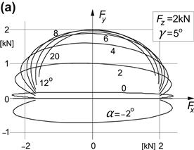
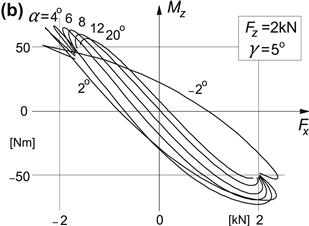
FIGURE 4.7 (a) Cornering force vs longitudinal force at a new load and camber angle as computed with the similarity method. (b) Aligning torque vs longitudinal force at a new load and camber angle as computed with the similarity method.
It may be further remarked that the similarity model given by Eqns (4.35–4.40) together with (4.27a, b), (4.28) and the reference pure slip functions does represent the actual tire steady-state behavior well in the following extreme cases: (1) in pure slip situations, (2) in the linearized combined slip situation (small α and κ), and (3) in the case of a locked wheel (at γ = 0). As illustrated in Figure 4.6, the model correctly shows that when the wheel is locked, the resulting force acts in a direction opposite to the slip speed vector Vs if, in the original reference pure slip curves, the level of Fxo and of Fyo tends to the same level when both slip components approach infinity (governed by the parameters μ and C in the Magic Formula). Other combinations of slip may give rise to deviations with respect to measured characteristics. It is noted that when the terms for the aligning torque with parameters c9, c10, and c11 are disregarded, the combined slip performance can be represented without the necessity to rely on combined slip measurement data.
A comparison with measured data is given in Figure 4.8. Here the similarity method is used where instead of the theoretical slip quantities the practical slip variables κ and tan α (that is: sx and sy) have been employed also in the derivation phase (in Eqns (4.35–4.38)). A relatively good agreement is achieved for this passenger car tire in the combined slip situation.
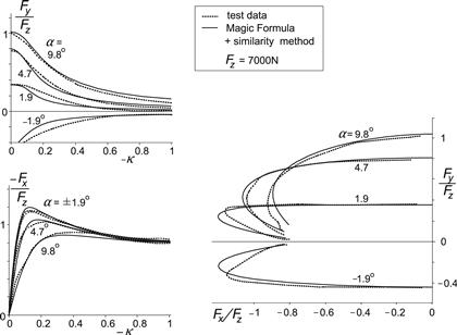
FIGURE 4.8 Tire combined slip characteristics as obtained from measurements with the Delft tire test trailer compared with the curves calculated with the aid of the similarity method.
4.2.3 Combined Slip Conditions with Fx as Input Variable
In simpler vehicle dynamics simulation studies with the wheel spin degree of freedom not included, one may prefer to use the longitudinal force Fx as input quantity instead of the longitudinal slip κ. This approach has been used, almost exclusively, in early vehicle dynamics research. However, for (quasi) steady-state cornering analysis, notably circuit simulation in the racing world, this option is still popular. An important limitation of using this method is the condition that the Fx vs κ characteristic (although not used) is supposed to show a positive slope over the entire range of longitudinal slip while at wheel lock Fx = −μFz, or, alternatively, we use only that part of the characteristic that lies in between the two peaks. This entails that the Fy vs Fx curves are single valued in the Fx range employed. Furthermore, it is assumed that the friction coefficient is the same for longitudinal and lateral directions and is denoted by μ.
The obvious main effect of the introduction of Fx on the side force is the lowering of the maximum side force that can be generated. For this to realize, the right-hand expressions of Eqns (4.23) and (4.25) are to be multiplied with the factor
![]() (4.41)
(4.41)
while expression (4.24) is to be divided by the same factor. The cornering and aligning stiffnesses remain unaffected through this operation. These stiffnesses, however, do depend on the longitudinal force, as becomes obvious from the curves of Figure 3.13 that belong to small side-slip angles. The following functions may serve as a crude approximation of the actual relationships:
![]() (4.42)
(4.42)
with
![]() (4.42a)
(4.42a)
Depending on the user’s desire, one may choose for n a value in the range of 2–8 (more or less curved characteristic CFα(Fx)). For the aligning stiffness, we may use the formula
![]() (4.43)
(4.43)
and, similar for the camber stiffness,
![]() (4.44)
(4.44)
The camber moment stiffness may be disregarded. The load dependencies CF,Mα(Fz) and CFγ(Fz) of the freely rolling tire already appeared in Eqns (4.24, 4.25). It may be ascertained that the present model makes sure that the cornering stiffness vanishes when Fx → μFz (wheel drive spin, κ → ∞) while at Fx = −μFz (wheel lock, κ = −1) the side-slip ‘stiffness’ equals μFz, which is correct. The functional relationships (4.21, 4.22) for Fx do not play a role anymore and the friction coefficient μy has been replaced by μ. The imposed longitudinal force should be kept within the boundaries ![]() .
.
The resulting equations for the side force and the aligning torque with the longitudinal force serving as one of the input quantities now read
For the side force,
![]() (4.45)
(4.45)
with the equivalent slip angle
![]() (4.46)
(4.46)
and, for the aligning torque,
![]() (4.47)
(4.47)
where the last terms have been taken from (4.39) and the residual torque reads
![]() (4.48)
(4.48)
Exercise 4.1 given at the end of Section 4.3 addresses the problem of assessing the side force characteristics using the similarity technique with the longitudinal force considered as one of the input quantities.
In Section 4.3, the Magic Formula tire model will be treated in detail. This complex model is considerably more accurate and will again employ the longitudinal slip κ as input variable.
4.3 The Magic Formula Tire Model
A widely used semi-empirical tire model to calculate steady-state tire force and moment characteristics for use in vehicle dynamics studies is based on the so-called Magic Formula. The development of the model was started in the mid-eighties. In a cooperative effort, TU-Delft and Volvo developed several versions (Bakker et al. 1987, 1989, Pacejka et al. 1993). In these models, the combined slip situation was modeled from a physical viewpoint. In 1993, Michelin (cf. Bayle et al. 1993) introduced a purely empirical method using Magic Formula-based functions to describe the tire horizontal force generation at combined slip. This approach has been adopted in subsequent versions of the Magic Formula Tire Model. In the newer version of the model, the original description of the aligning torque has been altered to accommodate a relatively simple physically based combined slip extension. The pneumatic trail is introduced as a basis to calculate this moment about the vertical axis, cf. Pacejka (1996). A complete listing of the model is given in Section 4.3.2. In Section 4.3.3, the model is further extended by introducing formulas for the description of the situation at large camber angle γ and turn slip φt.
4.3.1 Model Description
The general form of the formula, that holds for given values of vertical load and camber angle, reads
![]() (4.49)
(4.49)
with
![]() (4.50)
(4.50)
![]() (4.51)
(4.51)
where Y is the output variable Fx, Fy or possibly Mz and X the input variable tan α or κ, and B is the stiffness factor, C the shape factor, D the peak value, E the curvature factor, SH the horizontal shift, and SV the vertical shift.
The Magic Formula y(x) typically produces a curve that passes through the origin x = y = 0, reaches a maximum, and subsequently tends to a horizontal asymptote. For given values of the coefficients B, C, D, and E, the curve shows an anti-symmetric shape with respect to the origin. To allow the curve to have an offset with respect to the origin, two shifts SH and SV have been introduced. A new set of coordinates Y(X) arises as shown in Figure 4.9. The formula is capable of producing characteristics that closely match measured curves for the side force Fy (and if desired also for the aligning torque Mz) and for the fore-and-aft force Fx as functions of their respective slip quantities: the slip angle α and the longitudinal slip κ with the effect of load Fz and camber angle γ included in the parameters.
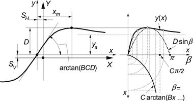
FIGURE 4.9 Curve produced by the original sine version of the Magic Formula, Eqn (4.49). The meaning of curve parameters has been indicated.
Figure 4.9 illustrates the meaning of some of the factors by means of a typical side force characteristic. Obviously, coefficient D represents the peak value (with respect to the central x-axis and for C ≥1) and the product BCD corresponds to the slope at the origin (x = y = 0). The shape factor C controls the limits of the range of the sine function appearing in formula (4.49) and thereby determines the shape of the resulting curve. The factor B is left to determine the slope at the origin and is called the stiffness factor. The factor E is introduced to control the curvature at the peak and, at the same time, the horizontal position of the peak.
From the heights of the peak and of the horizontal asymptote, the shape factor C may be computed:
![]() (4.52)
(4.52)
From B and C and the location xm of the peak, the value of E may be assessed:
![]() (4.53)
(4.53)
The offsets SH and SV appear to occur when ply-steer and conicity effects and possibly the rolling resistance cause the Fy and Fx curves not to pass through the origin. Wheel camber may give rise to a considerable offset of the Fy vs α curves. Such a shift may be accompanied by a significant deviation from the pure anti-symmetric shape of the original curve (cf. Figure 3.35c,d). To accommodate such an asymmetry, the curvature factor E is made dependent on the sign of the abscissa (x):
![]() (4.54)
(4.54)
Also, the difference in shape that is expected to occur in the Fx vs κ characteristic between the driving and braking ranges can be taken care of. In Figure 4.10, the influence of the two shape factors C and E on the appearance of the curves has been demonstrated. The diagrams have been normalized by dividing y by D and multiplying x with CB, making the curve peak level and initial slope independent of the parameters.
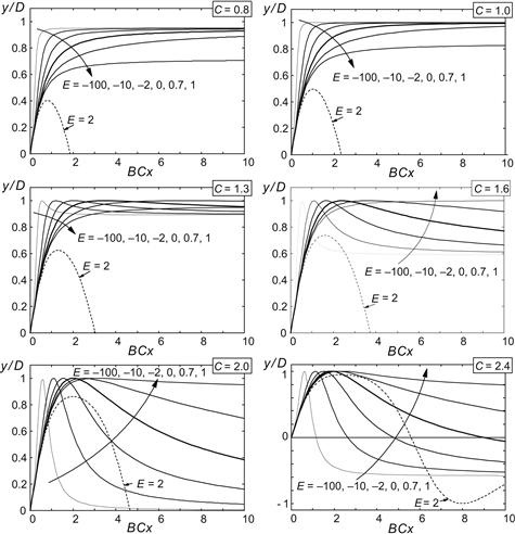
FIGURE 4.10 The influence of the shape factors C and E on the appearance of the curve according to Eqn (4.49). Note that a value of curvature factor E > 1 does not produce realistic curves.
In rather extreme cases, the sharpness that can be reached by means of the function given by Eqn (4.49) may not be sufficient. It turns out to be possible to considerably increase the sharpness of the curves by introducing an extra term in the argument of the arctan function. The modified function reads
![]() (4.55)
(4.55)
Figure 4.11 demonstrates the effect of the new coefficient H. Too large values may give rise to an upward curvature of the curve near the origin as would also occur at large negative values of E (cf. the lower diagrams of Figure 4.10). In the ensuing text, we will not use this additional coefficient H.
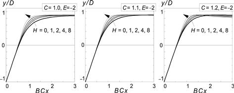
FIGURE 4.11 Sharpness of curves near the peak may be increased by introducing additional term with sharpness factor H (according to Eqn (4.55)).
It may be furthermore of interest to note that the possibly awkward function arctan(x) may be replaced by the possibly faster and almost identical pseudo-arctan function psatan(x) = x(1 + a|x|)/{1 + 2(b|x| + ax2)/π} with a = 1.1 and b = 1.6.
The various factors are functions of normal load and wheel camber angle. Several parameters appear in these functions. A suitable regression technique is used to determine their values from measured data according to a quadratic algorithm for the best fit (cf. Oosten and Bakker 1993). One of the important functional relationships is the variation of the cornering stiffness (almost exactly given by the product of coefficients By, Cy, and Dy of the side force function: BCDy = Kyα = ∂Fy/∂α at tan α = −SH) with Fz and γ:
![]() (4.56)
(4.56)
For zero camber, the cornering stiffness attains its maximum p1 at Fz = p2. In Figure 4.12, the basic relationship has been depicted. Apparently, for a cambered wheel, the cornering stiffness decreases with increasing |γ|. Note the difference in curvature left and right of the characteristics at larger values of the camber angle. To accomplish this, a split-E according to Eqn (4.54) has been employed. We refer to Section 4.3.2 for a complete listing of the formulas. Here, nondimensional parameters have been introduced. For example, the parameters in (4.56) will become: p1 = Fzo pKy1, p2 = Fzo pKy2, and p3 = pKy3, with Fzo denoting the nominal wheel load.
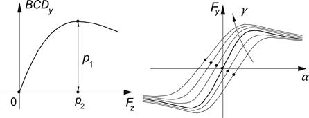
FIGURE 4.12 Cornering stiffness vs vertical load and the influence of wheel camber, Eqn (4.56).
The aligning torque Mz can now be obtained by multiplying the side force Fy with the pneumatic trail t and adding the usually small (except with camber) residual torque Mzr (cf. Figure 4.13). We have
![]() (4.57)
(4.57)
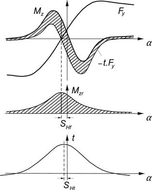
FIGURE 4.13 The aligning torque characteristic composed of a part directly attributed to the side force and a part due the so-called residual torque (due to tire conicity and camber).
For the differently defined side force ![]() , we refer to the remark below Eqn (4.74). The pneumatic trail decays with increasing side slip and is described as follows:
, we refer to the remark below Eqn (4.74). The pneumatic trail decays with increasing side slip and is described as follows:
![]() (4.58)
(4.58)
where
![]() (4.59)
(4.59)
The residual torque shows a similar decay:
![]() (4.60)
(4.60)
with
![]() (4.61)
(4.61)
It is observed that both parts of the moment are modeled using the Magic Formula, but instead of the sine function, the cosine function is employed. In that way, a hill-shaped curve is produced. The peaks are shifted sideways.
The residual torque is assumed to attain its maximum Dr at the slip angle where the side force becomes equal to zero. This is accomplished through the horizontal shift SHf. The peak of the pneumatic trail occurs at tan α = −SHt. This formulation has proven to give very good agreement with measured curves. The advantage with respect to the earlier versions, where formula (4.49) is used for the aligning torque as well, is that we have now directly assessed the function for the pneumatic trail which is needed to handle the combined slip situation.
In Figure 4.14, the basic properties of the cosine based curve have been indicated (subscripts of factors have been deleted again). Again, D is the peak value, C is a shape factor determining the level ya of the horizontal asymptote, and now B influences the curvature at the peak (illustrated with the inserted parabola). Factor E modifies the shape at larger values of slip and governs the location xo of the point where the curve intersects the x-axis. The following formulas hold:
![]() (4.62)
(4.62)
![]() (4.63)
(4.63)
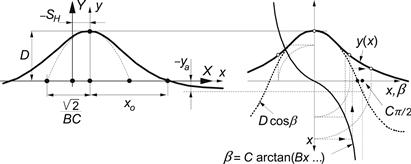
FIGURE 4.14 Curve produced by the cosine version of the Magic Formula, Eqn (4.58). The meaning of curve parameters has been indicated.
In the original version of the formula (4.57), cf. 1st or 2nd edition of this book, the force F y was used instead of F′y. The force F′y constitutes the side force due to only side slip. That is, with input camber (and turn slip) disregarded. In addition, the different form of the force function (4.49) specially introduced for the possibly at large camber operating motorcycle, has been abandoned. The new formulations are listed in Sec. 4.3.2 which can now be employed successfully for both car and motorcycle tyres. Also see discussion below Eq. (4.74).
In the case of the possible presence of large camber angles (motorcycles), it may be better to use in (4.57) the side force Fy that would arise at γ = 0. Also, the side force function (4.49) and the cornering stiffness function (4.56) may be mod-ified to better approximate large camber response for motorcycle tires, cf. De Vries (1998a) and Sec.11.6 for a full listing of equations. We refer to Section 4.3.3 for the discussion of the model extension for larger camber and turn slip (path curvature) also applicable in the case of combined slip with braking or driving forces.
In the paper of Pacejka and Bakker (1993), the tire’s response to combined slip was modeled by using physically based formulas. A newer more efficient way is purely empiric. This method was developed by Michelin and published by Bayle, Forissier, and Lafon (1993). It describes the effect of combined slip on the lateral force and on the longitudinal force characteristics. Weighting functions G have been introduced which, when multiplied with the original pure slip functions (4.49), produce the interaction effects of κ on Fy and of α on Fx. The weighting functions have a hill shape. They take the value one in the special case of pure slip (either κ or α equal to zero). When, for example, at a given slip angle a from zero increasing brake slip is introduced, the relevant weighting function for Fy may first show a slight increase in magnitude (becoming larger than one) but will soon reach its peak after which a continuous decrease follows. The cosine version of the Magic Formula is used to represent the hill shaped function:
![]() (4.64)
(4.64)
Here, G is the resulting weighting factor and x is either κ or tan α (possibly shifted). The coefficient D represents the peak value (slightly deviating from one if a horizontal shift of the hill occurs), C determines the height of the hill’s base, and B influences the sharpness of the hill. Coefficient B constitutes the main factor responsible for the shape of the weighting functions.
As an extension to the original function published by Bayle et al., the part with shape factor E will be added later on. This extension appears to improve the approximation, in particular at large levels of slip, especially in view of the strict condition that the weighting function G must remain positive for all slip conditions.
For the side force, we get the following formulas:
![]() (4.65)
(4.65)
with the weighting function now expressed such that it equals unity at κ = 0:
![]() (4.66)
(4.66)
where
![]() (4.67)
(4.67)
and further the coefficients
![]() (4.68a)
(4.68a)
![]() (4.68b)
(4.68b)
![]() (4.68c)
(4.68c)
![]() (4.69a)
(4.69a)
![]() (4.69b)
(4.69b)
with dfz the notation for the nondimensional increment of the vertical load with respect to the (adapted) nominal load, cf. next Subsection 4.3.2, Eqn (4.E2a). Figure 4.15 depicts the two weighting functions displayed as functions of both α and κ and the resulting force characteristics (parameters according to Table 4.2 on p. 190). Below, an explanation is given.
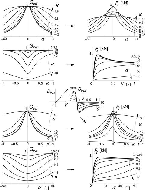
FIGURE 4.15 Nature of weighting functions and the resulting combined slip longitudinal and lateral forces, the latter also affected by the κ induced ply-steer ‘vertical shift’ SVyκ.
In Eqn (4.65) Fyo denotes the side force at pure side slip obtained from Eqn (4.49). The denominator of the weighting function (4.66) makes Gyκ = 1 at κ = 0. The horizontal shift SHyκ of the weighting function accomplishes the slight increase that the side force experiences at moderate braking before the peak of Gyκ is reached and the decay of Fy commences.
This horizontal shift may be made dependent on the vertical load. Cyκ controls the level of the horizontal asymptote. If Cyκ = 1, the weighting function (4.66) will approach zero when κ → ±∞. This would be the correct value for Cyκ if κ is expected to be used in the entire range from plus to minus infinity. If this is not intended, then Cyκ may be chosen different from one if Gyκ is optimized with the restriction to remain positive. The factor Byκ influences the sharpness of the hill shaped weighting function. As indicated, the hill becomes more flat (wider) at larger slip angles. Then Byκ decreases according to (4.68a). When in an extreme situation α approaches 90°, that is when Vcx → 0, Byκ will go to zero and, consequently, Gyκ will remain equal to one unless κ goes to infinity which may easily be the case when at Vcx → 0 the wheel speed of revolution Ω and thus the longitudinal slip velocity Vsx remain unequal to zero. The quantity SVyκ is the vertical ‘shift’, which sometimes is referred to as the κ-induced ply-steer. At camber, due to the added asymmetry, the longitudinal force clearly produces a torque that creates a torsion angle comparable with a possibly already present ply-steer angle. This shift function varies with slip κ indicated in (4.69a).
As illustrated in Figure 4.15, its peak value DVyκ depends on the camber angle γ and decays with increasing magnitude of the slip angle α. Figure 4.16 presents measured data together with the fitted curves as published by Bayle et al.
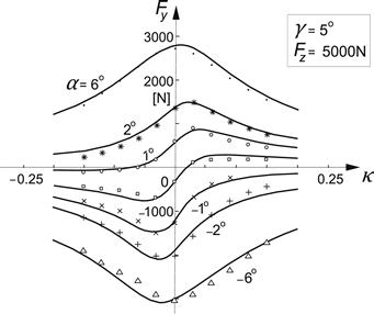
FIGURE 4.16 The combined side slip force characteristics in the presence of a camber angle, Bayle et al. (1993).
The combined slip relations for Fx are similar to what we have seen for the side force. However, a vertical shift function was not needed. In Figure 4.17, a three-dimensional graph is shown indicating the variation of Fx and Fy with both α and κ. The initial ‘S’ shape of the Fy vs κ curves (at small α) due to the vertical shift function is clearly visible.
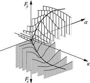
FIGURE 4.17 Three-dimensional graph of combined slip force characteristics.
For possible improvement of the general tendency of the model at larger levels of combined slip beyond the range of available test data, one might include additional ‘fabricated’ data which are derived from similarity method results at larger values of the slip angle. Another possibility is the usage of the conditions at wheel lock where one might assume that the force and slip vector are colinear. We then have, for the ratio of the components,
![]() (4.70)
(4.70)
or
![]() (4.71)
(4.71)
![]() (4.72)
(4.72)
Regarding the aligning torque, physical insight is used to model the situation at combined slip. We write
![]() (4.73)
(4.73)
The arguments αt and αr (including a shift) appearing in the functions (4.59, 4.61) for the pneumatic trail and residual torque at pure side slip are replaced by equivalent slip angles, as indicated by Eqn (4.74), incorporating the effect of κ on the composite slip:
![]() (4.74)
(4.74)
and similar for αr,eq. To approximate the same effect on the degree of sliding in the contact patch as would occur with side slip, the longitudinal slip κ is multiplied with the ratio of the longitudinal and lateral slip stiffnesses.
Besides, an extra term is introduced in (4.73) to account for the fact that a moment arm s arises for Fx as a result of camber γ and lateral tire deflection related to Fy. This extra term may give rise to a sign change of the aligning torque in the range of braking as discussed before (cf. Figure 3.20).
With respect to the previous version of the expression for the aligning torque, presented in e.g., the 2nd edition of this book, an important change has been introduced that originates from the special version developed for the motorcycle tire (MC-MF tire) that can handle large camber angles, cf. 2nd edition and De Vries and Pacejka (1998a). In the first term of Eqn (4.73), the full side force Fy has been replaced by the side force ![]() that is generated by only the side-slip angle α (possibly influenced by the fore-and-aft slip κ). Consequently,
that is generated by only the side-slip angle α (possibly influenced by the fore-and-aft slip κ). Consequently, ![]() results from
results from ![]() calculated with γ = φt = 0. With this replacement, the full set of equations, presented in the next Subsection 4.3.2, is now capable of accurately modeling force and moment response for both car and motorcycle tires. Note that this replacement is more logical because γ and φt cause almost symmetrical lateral deflections. The accompanying moment Mzr arises through anti-symmetric longitudinal tread deflections. The replacement might, however, be partially disturbed through an Mzr-induced slip angle (contact patch torsion through carcass torsional compliance). This makes the lateral deflection a little less symmetric.
calculated with γ = φt = 0. With this replacement, the full set of equations, presented in the next Subsection 4.3.2, is now capable of accurately modeling force and moment response for both car and motorcycle tires. Note that this replacement is more logical because γ and φt cause almost symmetrical lateral deflections. The accompanying moment Mzr arises through anti-symmetric longitudinal tread deflections. The replacement might, however, be partially disturbed through an Mzr-induced slip angle (contact patch torsion through carcass torsional compliance). This makes the lateral deflection a little less symmetric.
At the end of this chapter, force and moment characteristics for car, truck, and motorcycle tires as computed with the Magic Formula equations have been presented. They are compared with curves that result from steady-state full-scale tire tests.
4.3.2 Full Set of Equations
The complete set of steady-state formulas contains nondimensional parameters p, q, r, and s. In addition, user scaling factors λ have been introduced. With that tool, the effect of changing friction coefficient, cornering stiffness, camber stiffness, etc., can be quickly investigated in a qualitative way without having the need to implement a completely new tire data set. Scaling is done in such a way that realistic relationships are maintained. For instance, when changing the cornering stiffness and the friction coefficient in lateral direction (through λKyα and λμy), the abscissa of the pneumatic trail characteristic is changed in a way equal to that of the side force characteristic and in accordance with the similarity method of Section 4.2.
The Magic Formula model equations listed below are in accordance with the description given in the MF-Tire/MF-Swift 6.1.2 Equation Manual, cf. TNO Automotive (2010). The equations contain the nondimensional model parameters p, q, r, and s and, in addition, a set of scaling factors λ. Other parameters and variable quantities used in the equations are:
| g | acceleration due to gravity, |
| Vc | magnitude of the velocity of the wheel contact center C, |
| Vcx,y | components of the velocity of the wheel contact center C, |
| Vsx,y | components of slip velocity Vs (of point S) with Vsy ≈ Vcy, Eqn (2.13), |
| Vr | (=Re Ω = Vcx − Vsx) forward speed of rolling, |
| Vo | reference velocity (=√(g Ro) or other specified value), |
| Ro | unloaded tire radius (=ro), |
| Re | effective rolling radius (=re), |
| Ω | wheel speed of revolution, |
| ρz | tire radial deflection (>0 if compression), and |
| Fz | normal load (= FN ≥ 0). Note: in Chaps. 9 and 10 Fz = −FN (≤0): |
| nominal (rated) wheel load, | |
| adapted nominal load, | |
| pi | tire inflation pressure, and |
| pio | nominal inflation pressure. |
The effect of having a tire with a different nominal load may be roughly approximated by using the scaling factor λFzo:
![]() (4.E1)
(4.E1)
Further, we introduce the normalized change in vertical load
![]() (4.E2a)
(4.E2a)
and similarly the normalized change in inflation pressure:
![]() (4.E2b)
(4.E2b)
The approximate influence of a change in inflation pressure as assessed through numerous tire tests has been recently investigated and introduced in the Magic Formula model equations, cf. Besselink et al. (2009).
Instead of taking the slip angle α itself (in radians, from Eqn (2.12)) as input quantity, one may, in the case of very large slip angles and possibly backwards running of the wheel, better use the tangent of the slip angle defined as the lateral slip:
![]() (4.E3)
(4.E3)
For the spin due to the camber angle, we introduce
![]() (4.E4)
(4.E4)
The longitudinal slip ratio is defined as follows:
![]() (4.E5)
(4.E5)
If the forward speed Vcx becomes or is equal to zero, one might add a small quantity ε in the denominator of (4.E3, 4.E5) to avoid singularity, or, when transient slip situations occur, one should use the transient slip quantities (or deformation gradients) tan α′ and κ′ as defined and used in Chapters 7 and 8.
To avoid the occurrence of similar singularities in the ensuing equations due to e.g., zero velocity or zero vertical load, a small additional quantity ε (with same sign as its neighboring main quantity) will be introduced in relevant denominators like in the next equation.
For the factor cos α appearing in the equations for the aligning torque to properly handle the case of large slip angles and possibly backwards running (Vcx < 0), we have defined
![]() (4.E6)
(4.E6)
![]() (4.E6a)
(4.E6a)
where we may choose ![]() .
.
For the normally encountered situations where turn slip φt may be neglected (path radius R → ∞) and camber remains small, the factors ζi appearing in the equations may be set equal to unity:
![]()
In the following Subsection 4.3.3 where the influence of spin (turn slip and camber) is discussed, the proper expressions will be given for the factors ζi, and additional equations will be introduced.
User Scaling Factors
The following set of scaling factors λ is available. The default value of thesefactors is set equal to one (except λμV which equals zero if not used). We have:
λμx,y peak friction coefficient
λμV with slip speed Vs decaying friction
To change from a relatively high friction surface to a low friction surface, the factors λμx and λμy may be given a value lower than unity. In addition, to reflect a slippery surface (wet) with friction decaying with increasing (slip) speed, one may choose for λμV a value larger than zero, e.g., Eqns (4.E13, 4.E23). The publications of Dijks (1974) and of Reimpell et al. (1986) may be useful in this respect. Note that the slip stiffnesses are not affected through these changes. For the composite friction scaling factor, in x- and y-direction respectively, we have
![]() (4.E7)
(4.E7)
A special degressive friction factor ![]() is introduced to recognize the fact that vertical shifts of the force curves do vanish when μ → 0 but at a much slower rate:
is introduced to recognize the fact that vertical shifts of the force curves do vanish when μ → 0 but at a much slower rate:
![]() (4.E8)
(4.E8)
For the three forces and three moments acting from road to tire and defined according to the diagram of Figure 2.3, the equations, first those for the condition of pure slip (including camber) and subsequently those for the condition of combined slip, read (version 2004).
Longitudinal Force (Pure Longitudinal Slip, α = 0)
![]() (4.E9)
(4.E9)
![]() (4.E10)
(4.E10)
![]() (4.E11)
(4.E11)
![]() (4.E12)
(4.E12)
![]() (4.E13)
(4.E13)
![]() (4.E14)
(4.E14)
 (4.E15)
![]() (4.E16)
(4.E16)
![]() (4.E17)
(4.E17)
![]() (4.E18)
(4.E18)
Lateral Force (Pure Side Slip, κ = 0)
![]() (4.E19)
(4.E19)
![]() (4.E20)
(4.E20)
![]() (4.E21)
(4.E21)
![]() (4.E22)
(4.E22)
![]() (4.E23)
(4.E23)
![]() (4.E24)
(4.E24)
![]() (4.E25)
(4.E25)
![]() (4.E26)
(4.E26)
![]() (4.E27)
(4.E27)
![]() (4.E28)
(4.E28)
![]() (4.E29)
(4.E29)
![]() (4.E30)
(4.E30)
Aligning Torque (Pure Side Slip, κ = 0)
![]() (4.E31)
(4.E31)
![]() (4.E32)
(4.E32)
![]() (4.E33)
(4.E33)
![]() (4.E34)
(4.E34)
![]() (4.E35)
(4.E35)
![]() (4.E36)
(4.E36)
![]() (4.E37)
(4.E37)
![]() (4.E38)
(4.E38)
![]() (4.E39)
(4.E39)
![]() (4.E40)
(4.E40)
![]() (4.E41)
(4.E41)
![]() (4.E42)
(4.E42)
![]() (4.E43)
(4.E43)
![]() (4.E44)
(4.E44)
![]() (4.E45)
(4.E45)
![]() (4.E46)
(4.E46)
![]() (4.E47)
(4.E47)
![]() (4.E48)
(4.E48)
![]() (4.E49)
(4.E49)
Longitudinal Force (Combined Slip)
![]() (4.E50)
(4.E50)
![]() (4.E51)
(4.E51)
![]() (4.E52)
(4.E52)
![]() (4.E53)
(4.E53)
![]() (4.E54)
(4.E54)
![]() (4.E55)
(4.E55)
![]() (4.E56)
(4.E56)
![]() (4.E57)
(4.E57)
Lateral Force (Combined Slip)
![]() (4.E58)
(4.E58)
![]() (4.E59)
(4.E59)
![]() (4.E60)
(4.E60)
![]() (4.E61)
(4.E61)
![]() (4.E62)
(4.E62)
![]() (4.E63)
(4.E63)
![]() (4.E64)
(4.E64)
![]() (4.E65)
(4.E65)
![]() (4.E66)
(4.E66)
![]() (4.E67)
(4.E67)
Normal Load (see also Eqns (7.48) and (9.217))
![]() (4.E68)
(4.E68)
Overturning Couple (also see Section 4.3.5)
![]() (4.E69)
(4.E69)
Rolling Resistance Moment (see Eqns (9.236, 9.230, 9.231))
![]() (4.E70)
(4.E70)
Aligning Torque (combined slip)
![]() (4.E71)
(4.E71)
![]() (4.E72)
(4.E72)
![]() (4.E73)
(4.E73)
![]() (4.E74)
(4.E74)
![]() (4.E75)
(4.E75)
![]() (4.E76)
(4.E76)
![]() (4.E77)
(4.E77)
![]() (4.E78)
(4.E78)
Note that actually −SHxCFκ should equal My/rl making κ = 0 at free rolling (drive torque MD = 0). If SHx is set equal to zero, κ vanishes at MD = My, making Fx =0.
A set of parameter values has been listed in App. 3 for an example tire in connection with the SWIFT tire model to be dealt with in Chapter 9. Examples of computed characteristics compared with experimentally assessed curves for both pure slip and combined slip conditions are discussed in Section 4.3.6, cf. Figures 4.28–4.34. In Section 4.3.3, the effect of having turn slip is modeled and some calculated characteristics have been presented for a set of hypothetical model parameters (Figure 4.19). Section 4.3.4 examines the possibility to define the effects of conicity and ply-steer as responses to equivalent camber and slip angles. Section 4.3.5 gives the basis for the expression Eqn (4E.69) of the overturning couple of truck, car, and racing tires due to side slip and provides a discussion on the part due to camber.
4.3.3 Extension of the Model for Turn Slip
The model described so far contains the input slip quantities side slip, longitudinal slip, and wheel camber. In the present section, the turn slip or (in steady state) path curvature is added which completes the description of the steady-state force and moment generation properties of the tire.
Turn slip is one of the two components which together form the spin of the wheel, cf. Figure 3.22. The turn slip is defined as (last equality, with R the turn radius, is valid only if the side-slip angle α remains zero or constant)
![]() (4.75)
(4.75)
and the total tire spin, cf. Eqn (3.55):
![]() (4.76)
(4.76)
with the singularity protected velocity ![]() . Again, εγ denotes the camber reduction factor for the camber to become comparable with turn slip. For radial-ply car tires, this reduction factor εγ may become as high as ca. 0.7 (for some truck tires even slightly over 1.0), while for a motorcycle tire the factor is expected to be close to zero as with a homogeneous solid ball, cf. discussion below Eqn (3.117).
. Again, εγ denotes the camber reduction factor for the camber to become comparable with turn slip. For radial-ply car tires, this reduction factor εγ may become as high as ca. 0.7 (for some truck tires even slightly over 1.0), while for a motorcycle tire the factor is expected to be close to zero as with a homogeneous solid ball, cf. discussion below Eqn (3.117).
In the previous section, the effect of camber was introduced. For the side force, this resulted in a horizontal and a vertical shift of the Fy vs α curves, while for the aligning torque, besides the small effect of the shifted Fy curve, the residual torque Mzr was added in which a contribution of camber occurs. Furthermore, changes in shape appeared to occur which were represented by the introduction of γ in factors such as μy, Ey, Kyα, Bt, Dt, etc. These changes may be attributed to changes in tire cross section and contact pressure distribution resulting from the wheel inclination angle.
These shifts and shape changes will be retained in the model extension but will be expanded to cover the complete range of spin in combination with side slip and also longitudinal slip. The spin may change from zero to ±∞ when path curvature goes to infinity and, consequently, path radius to zero (when the velocity Vc → 0). Weighting functions will again be introduced to gradually reduce peak side and longitudinal forces with increasing spin. Also, cornering stiffness and pneumatic trail will be subjected to such a reduction.
The theoretical findings which have been gained from the physical model of Section 3.3 presented in Figure 3.35d will be used as basis for the model development. Since these findings hold for only one value of the vertical load and zero longitudinal slip, the influence of load variations and longitudinal slip has been structured tentatively.
In Figure 4.18 for the two extreme cases of α = 0 and α = 90°, the courses of Fy and Mz vs aφt =−a/R have been depicted. The pure spin side force characteristic shown in the left-hand diagram (at α = 0), also indicated in the lower left diagram of Figure 3.35d, can be fabricated by sideways shifting of the side force curve belonging to zero spin (turn slip φt = 0 and γ = 0, upper or middle left diagram) while at the same time reducing its peak value Dy and its slope at the curve center Kyα. For this, we define the reduction functions to be substituted in the previous Eqns (4.E22, 4.E25, 4.E28, 4.E29). The peak side force reduction factor (note: Ro here denotes the unloaded tire radius!)
![]() (4.77)
(4.77)
![]() (4.78)
(4.78)
and the slope reduction factor
![]() (4.79)
(4.79)
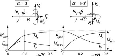
FIGURE 4.18 Two basic spin force and moment diagrams.
Herewith, the condition is satisfied that at φt →∞, where the wheel is steered about the vertical axis at a speed of travel equal to zero (that is: velocity of contact center Vc → 0 and path radius R → 0, leading to ζ2 = ζ3 = 0), the side force reduces to zero although a slip angle may theoretically still exist. Considering the upper- or middle-left diagram of Figure 3.35d, it seems that the sideways shift saturates at larger values of spin. To model this phenomenon, which actually says that beyond a certain negative slip angle no spin is large enough to make the side force vanish, the sine version of the Magic Formula is used. We have
![]() (4.80)
(4.80)
The shape factor CHyφ is expected to be equal or smaller than unity. To expression (4.80) is added the shift due to ply-steer and conicity. Finally, we subtract the horizontal displacement of the point of intersection of the side force vs slip angle curve which arises due to the vertical shift of the curve (which for now is thought to be solely attributed to the camber component of spin). This leads to a total horizontal shift:
![]() (4.81)
(4.81)
in which the vertical shift due to γ reads
![]() (4.82)
(4.82)
cf. Eqn (4.E28). The quantity ![]() is the singularity-protected cornering stiffness defined by Eqn (4.E39). Through this manipulation, the camber/spin stiffness is solely attributed to the horizontal shift of the point of intersection SHyφ, cf. Eqns (4.88, 4.89). Apparently, the factors ζ in Eqn (4.E27) now read
is the singularity-protected cornering stiffness defined by Eqn (4.E39). Through this manipulation, the camber/spin stiffness is solely attributed to the horizontal shift of the point of intersection SHyφ, cf. Eqns (4.88, 4.89). Apparently, the factors ζ in Eqn (4.E27) now read
![]() (4.83)
(4.83)
![]() (4.84)
(4.84)
The various factors appearing in (4.80) are defined as follows:
![]() (4.85)
(4.85)
![]() (4.86)
(4.86)
![]() (4.87)
(4.87)
![]() (4.88)
(4.88)
where the spin force stiffness KyRφo is related to the camber stiffness Kyγo (= CFγ) that is given by (4.E30):
![]() (4.89)
(4.89)
for which we may define
![]() (4.90)
(4.90)
Obviously, this parameter governs the difference of the response to camber with respect to that of turn slip.
For modeling the aligning torque, we will use as before the product of the side force and the pneumatic trail in the first term of Eqns (4.E31, 4.E71), while for the second term the residual torque will be expanded to represent large spin torque.
The middle-right diagram of Figure 3.35d shows that at increasing turn slip the residual or spin torque increases while the moment due to side slip (clearly visible at φt = 0) diminishes. This decay is modeled by means of the weighting function ζ5 multiplied with the pneumatic trail in Eqn (4.E43):
![]() (4.91)
(4.91)
The second term of Eqns (4.E31, 4.E71), the residual torque, which in the present context may be better designated as the spin moment, is given by Eqns (4.E36, 4.E75). Its peak value Dr has an initial value due to conicity that is expected to be taken over gradually by an increasing turn slip. In (4.E47), this is accomplished by the weighting function ζ2(4.77). The remaining terms will be replaced by the peak spin torque Drφ. This means that the ζ’s appearing in (4.E47) become, according to (4.83),
![]() (4.92)
(4.92)
As observed in the middle-right diagram of Figure 3.35d, the peak torque (that will be assumed to occur at a slip angle α = −SHf where Fy =0) grows with increasing spin and finally saturates. The Magic Formula describes this as follows:
![]() (4.93)
(4.93)
Its maximum value (if CDrφ ≥1) is DDrφ. The asymptotic level of the peak spin torque is reached at φ → ∞ or R → 0, and is denoted as Mzφ∞. Consequently, with the shape factor CDrφ, the maximum value is expressed by
![]() (4.94)
(4.94)
where the moment Mzφ∞ that occurs at vanishing wheel speed and at constant turning about the vertical axis is formulated as a function of the normal load:
![]() (4.95)
(4.95)
This expression may be compared with or replaced by expression (3.117) formulated by Freudenstein (1961). The shape factors in (4.93) are assumed to be given by constant parameters:
![]() (4.96)
(4.96)
![]() (4.97)
(4.97)
while
![]() (4.98)
(4.98)
with Kzγro assumed to depend on the normal load as follows:
![]() (4.99)
(4.99)
As has been indicated with Eqn (4.E49), we have, now for the camber moment stiffness,
![]() (4.100)
(4.100)
and consequently for the moment stiffness against spin:
![]() (4.101)
(4.101)
Now that the formulas for the peak of the spin torque Drφ have been developed, we must consider the remaining course of Mzr with the slip angle α. For this, Eqn (4.E36) is employed. According to the middle-right diagram of Figure 3.35d, the curves become flatter as the spin increases. Logically, for φ → ∞ the moment should become independent of the slip angle. The sharpness is controlled by the factor Br which we let gradually decrease to zero with increasing spin. For this, we introduce in Eqn (4.E45) the weighting function:
![]() (4.102)
(4.102)
The factor Cr controls the asymptotic level which corresponds to the torque at α = 90°. In that situation, the turn slip ![]() which corresponds to the definition given by Eqn (4.76). The moment Mzφ90 that is generated when the wheel moves at α = 90° increases with increasing curvature 1/R up to its maximum value that is attained at R = 0 and equals Mzφ∞. We use the formula
which corresponds to the definition given by Eqn (4.76). The moment Mzφ90 that is generated when the wheel moves at α = 90° increases with increasing curvature 1/R up to its maximum value that is attained at R = 0 and equals Mzφ∞. We use the formula
![]() (4.103)
(4.103)
with parameter qCrφ2. This quantity may be difficult to assess experimentally; the value 0.1 is expected to be a reasonable estimate. (In any case, the argument of (4.104) should remain <1.) This moment at 90° is multiplied with the weighting function Gyκ (4.E59) to account for the attenuation through the action of longitudinal slip.
We obtain, for the factor ζ7 = Cr in Eqn (4.E46) using (4.E36) with |αr| → ∞,
![]() (4.104)
(4.104)
Finally, we must take care of the weighting function ζ1 which is introduced in the expressions (4.E12, 4.E18) for Fx to let the longitudinal force diminish with increasing spin. We define
![]() (4.105)
(4.105)
with
![]() (4.106)
(4.106)
With the factors ζ0, ζ1,…ζ8 determined and substituted in the Eqns (4.E9–4.E78), the description of the steady-state force and moment generation has been completed. To show that the formulas produce qualitatively correct results, a collection of computed curves has been presented in the diagrams of Figure 4.19. In Table 4.2the values of the model parameters have been listed. The diagrams show that the formulas are perfectly capable to at least qualitatively approximate the curves that have been computed with the brush simulation model of Chapter 3 (cf. Figure 3.35). It has not been attempted to find a best fit for the parameters.
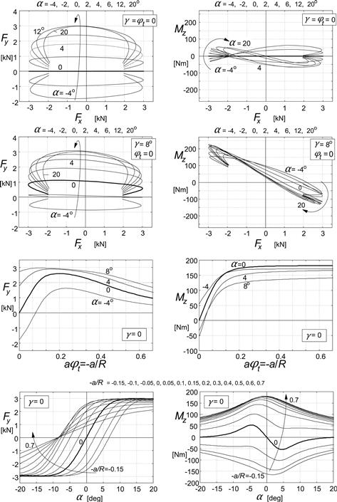
FIGURE 4.19 Magic Formula results for steady-state response of forces Fx,y and moment Mz to slip angle α, slip ratio κ, camber angle γ, and nondimensional path curvature φt = −a/R.
TABLE 4.2 Magic Formula Hypothetical Model Parameter Values for Diagrams of Figure 4.19. Parameters that Govern the Influence of Longitudinal Slip and Changes in Vertical Load have been given the Value Zero
4.3.4 Ply-Steer and Conicity
In the formulas for the side force Fy and the aligning torque Mz, the vertical shift SVy, the horizontal shift SHy, and the residual torque peak value Dr contain terms which produce the initial values of side force and aligning torque that occur at straight ahead running (at α = 0). These initial values are known to be the result of conicity and ply-steer, which are connected with nonsymmetry of the tire construction. These two possible sources result in markedly different behavior of the tire when, at geometrically zero side slip, the tire is rolled forward or backward. If we would have a tire that exhibits ply-steer but no conicity, the generated side force will point to the opposite direction when the wheel is changed from forward to backward rolling. This would also be the case when on a test rig the wheel moves at a small steer angle ψ and the road surface motion is changed from backward to forward. For that reason, ply-steer is sometimes referred to as pseudo-side-slip. If, on the other hand, the tire would show pure conicity, the side force will remain pointing in the same direction when the wheel is rolled in the opposite direction. This behavior is similar to that of a cambered wheel, which explains the term: pseudo-camber. In Figure 4.20 for the different cases, the diagrams for the side force variation resulting from yaw angle variations have been depicted. The curved or skewed foot prints of the tire that due to nonsymmetric construction of carcass and belt would arise on a zero friction surface explains the resulting characteristics. Definitions of conicity and ply-steer follow from the forces found at zero steer angle ψ.
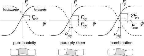
FIGURE 4.20 Side force vs steer angle characteristics at forward and backward rolling showing the cases of pure conicity, pure ply-steer, and a combination of both situations. Below, the associated foot prints on a frictionless surface have been depicted.
The deformations of the tire rolling on a friction surface resemble those that would occur with a tire (free of conicity and ply-steer) that rolls at a small camber and side slip angle, respectively. It is therefore tempting to assume that in these comparable cases the moment Mz and the force Fy respond at the same rate which would mean that the associated pneumatic trails are equal for ply-steer and side slip and for conicity and camber. The assumption is partly supported by an extensive experimental investigation of Lee (2000), which assessed a strong linear correlation between conicity and the difference between slip angles where Fy and Mz become equal to zero. In Figure 4.21, this difference is designated as δo. Lee found that at δo = 0 conicity is almost zero. This means that for vanishing conicity the remaining ply-steer produces a moment that is approximately equal to minus the pneumatic trail for side slip times the side force. With the introduction of the (small) equivalent slip angle αply, we have
![]() (4.107)
(4.107)
and
![]() (4.108)
(4.108)
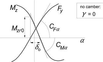
FIGURE 4.21 The situation near zero slip angle, force, and moment due to conicity and ply-steer.
Also according to Lee, the residual torque at zero side force, Mzr0 in Figure 4.21, is strongly correlated with δo and thus with conicity. We find, from the diagram,
![]() (4.109)
(4.109)
If we may further assume that for the conicity force and moment a similar correspondence with camber response exists, we would have after introducing an equivalent camber angle γcon:
![]() (4.110)
(4.110)
where tγ (>0) represents the distance of the point of application of the resulting camber thrust in front of the contact center (that is: negative trail). The conicity force becomes
![]() (4.111)
(4.111)
With these assumptions, it is possible to estimate the contributions of ply-steer and conicity in the initial values of side force and aligning torque (at α = γ = 0) from a set of tire parameters that belongs to one direction of rolling.
This enables the vehicle modeler to switch easily from the set of parameter values of the tire model that runs on the left-hand wheels of a car to the set for the right-hand wheels. To accomplish this, the equivalent camber parts of the left-hand tire model must be changed in sign for both the aligning moment and the side force to make the model suitable for the right-hand tire. Also, it is then easy to omit e.g., all conicity contributions which were originally present in the tire from which the parameters have been assessed through the fitting process.
To develop the theory, we will first consider the case of a tire without ply-steer and conicity and study the situation when a camber angle is applied. This condition is reflected by the diagram of Figure 4.22. Considering the relations entered in this figure, we may write, for the distance δγ,
![]() (4.112)
(4.112)
and consequently we can find the camber angle γ from the distance δγ. In a similar fashion, the conicity will be assessed in terms of the equivalent camber angle and after that, the part attributed to ply-steer can be determined and expressed in terms of the equivalent slip angle. Figure 4.23 illustrates the conversion to equivalent angles. We find, similar to the inverse of (4.112),
![]() (4.113)
(4.113)
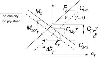
FIGURE 4.22 Characteristics of a tire without ply-steer or conicity near the origin at α = 0, with and without camber.
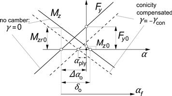
FIGURE 4.23 Characteristics of a tire with ply-steer and conicity showing conversion to equivalent camber and slip angle.
The equivalent slip angle can now be obtained from
![]() (4.114)
(4.114)
The four slip and camber stiffnesses are available from Eqns (4.E25, 4.E30, 4.E48, 4.E49). The sign of the forward velocity has been properly introduced.
The next thing we have to do is expressing δo and Δαo in terms of the shifts and the initial residual torque as defined in Section 4.3.2. We obtain, with (4.E38),
![]() (4.115)
(4.115)
and, from (4.109) and Figure 4.23,
![]() (4.116)
(4.116)
with CMα according to Eqn (4.E48) and the initial residual torque from (4.E47):
![]() (4.117)
(4.117)
Finally, the initial side force and torque are to be removed from the equations by putting the parameters pHy1, pHy2, pVy1, pVy2, qDz6, and qDz7 or the scaling factors λHy, λVy, and λMr equal to zero and by replacing in Eqns (4.E20, 4.E37) the original side slip input variable α∗ = tan α·sgnVcx by its effective value:
![]() (4.118)
(4.118)
and, in Eqns (4.E27, 4.E28, 4.E47) the original camber, γ∗ = sin γ by the effective total camber:
![]() (4.119)
(4.119)
where it should be realized that both αply and γcon are small quantities. The resulting diagram of Figure 4.24 shows characteristics that pass through the origin when the effective camber angle is equal to zero. For the tire running on the other side of the vehicle, the same model can be used but with γcon in (4.119) changed in sign.
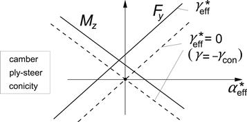
FIGURE 4.24 The final diagram with effective side slip and camber variables.
The theory above is based on considerations near the origin of the side force and aligning torque vs slip angle diagrams. The introduction of effective slip and camber angles may, however, give rise to slight changes in peak levels of the side force and probably also of the aligning torque. For the former, the situation may be repaired by moving the force characteristic in a direction parallel to the tangent at Fy = 0 resulting in an additional vertical shift:
![]() (4.120)
(4.120)
and an associated additional horizontal shift:
![]() (4.121)
(4.121)
Tire Pull
If identical tires would be fitted on the front axle of an automobile but with the conicity forces pointing in the same direction, and the vehicle moves along a straight line (that is: side forces are equal to zero), a steering torque must be applied that opposes the residual torques Mzr0 generated by the front tires (Figure 4.21). This is actually only approximately true because we may neglect the trails connected with ply-steer and conicity with respect to the vehicle wheel base. (In reality we have a small couple acting on the car exerted by the equal but opposite side forces front and rear which counteract the small, mainly conicity, torques front, and rear.) The phenomenon that a steer torque must be applied when moving straight ahead is called tire or vehicle pull. If the steering wheel would be released, the vehicle will deviate from its straight path.
If on the right-hand wheel a tire is mounted that is identical with the left-hand tire, one would actually expect that the conicity forces are directed in opposite directions and neutralize each other (as will occur also with the moments). This is because of the observation that one might compare the condition on the right-hand side with an identical tire rolling backward with respect to condition of the left-hand tire. In contrast, the ply-steer forces of the left and right tires act in the same direction but are compensated by side forces that arise through a small slip angle of the whole vehicle.
If the ply-steer angles, front and rear, are not the same, a small steer angle of the front wheels equal to the difference of the ply-steer slip angles front and rear is required for the vehicle to run straight ahead. The whole vehicle will run at a slip angle equal to that of the rear wheels.
4.3.5 The Overturning Couple
The overturning couple is especially important to investigate the vehicle roll-over occurrence and the curving behavior of a motorcycle. In moderate conditions, Eqn (4.E69) may often be sufficient to model the overturning moment. In the present section, we will study cases that require more elaborate modeling. The overturning couple is generated through the action of the side force and due to the camber angle. Eqn (4.E69) gives an expression valid for the combination of both components, further developed by TNO Automotive.
Due to Side Slip
Experience with measuring truck tires, racing tires, and passenger car tires shows that a positive overturning couple arises especially at low vertical loads as a response to positive side slip (situation depicted in Figure 4.25) while camber remains zero. This is probably in contrast to the behavior of narrow passenger car or motorcycle tires where, due to the lateral deflection connected with the side force Fy, the point of application of the resultant vertical force Fz moves in the direction of the side force and as a result generates a negative couple Mx. The observation that a tire may show a positive moment is expected to be connected with the belt that is stiff in torsion in the contact zone. This high stiffness opposes the flattening of the belt to remain in contact with the road when the belt is tilted through the action of the side force. This will especially be true when the contact patch is short, that is, at low load. As a result, the resultant vertical force vector will move more toward the edge away from the side force which causes the contact pressure to become relatively high on that side of the contact patch, thereby enabling the overturning couple to become positive. At higher loads, the middle portion of the belt contact range will show less resistance to remain horizontal and the overturning couple may turn to the more common negative values. It is of importance to note that the positive overturning couple at low loads and the ensuing sign change is observed to occur when measurements are conducted on, e.g., a flat plank or flat track machine where the axle height is recorded accurately and in the processing stage proper account is given to the standard definition of the overturning couple, that is the moment about the line of intersection of wheel center plane and ground plane. If the change in loaded radius is disregarded as is often done in past practice when measuring with over the road test vehicles, the positive part and the connected sign change is not observed. Consequently, it is of crucial importance that the tire test engineer and the vehicle dynamicist take care of employing, at least, the same definition for the overturning couple.
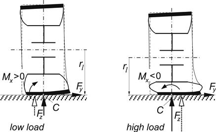
FIGURE 4.25 Tire at low load and at high load subjected to side slip giving rise to an overturning couple that may be of opposite sign.
The phenomenon may in some way be connected with the negative camber stiffness that is observed to occur with some type of tires also especially at low loads turning to positive at higher loads. The negative camber force generally changes to positive values when the camber angle becomes sufficiently large. At moderate loads, this also appears to happen with the overturning couple changing from positive to negative values at larger slip angles, that is: at higher side forces. The overturning couple response to wheel camber is always negative as might be expected. Obviously, the associated camber moment stiffness to be defined as CMxγ = −∂Mx/∂γ at zero camber is positive.
To model such a sign changing situation, the overturning couple response to side slip of the wheel is taken as an example. We will use a formula that is established by adding two functions:
![]() (4.122)
(4.122)
with the two contributions to the moment arm:
![]() (4.123)
(4.123)
![]() (4.124)
(4.124)
The first term y1 increases with the side force. The second term y2 grows, at least initially, with −Fy and diminishes with vertical load Fz. For the parameter values listed in Table 4.3, also containing assumed parameters for the side force characteristic, Eqns (4.E19–4.E26), the overturning couple has been calculated. Figure 4.26 shows the resulting curves. The same tendencies have been found to occur both with truck tires and passenger car tires. For the latter, we may refer to the diagram given in Figure 4.30. The same figure, which has been reproduced from the dissertation of Van der Jagt (2000), contains the diagram showing the decrease of the loaded radius with slip angle. This information is needed to assess the moment about the longitudinal axis through the wheel center. In Chapter 9, a formula is given which assumes that the decrease of the loaded radius is proportional to the squares of the lateral and the longitudinal deflections of the carcass, cf. Eqn (9.222). Experiments indicate that also the tire vertical stiffness is affected by horizontal tire forces, cf. Reimpell (1986), Eqn (9.217).
TABLE 4.3 Parameter Values for Overturning Couple Computation, cf. Eqns (4.120–4.122)
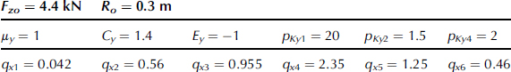
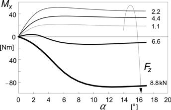
FIGURE 4.26 Overturning couple calculated with formulas (4.122–4.124), cf. Figure 4.30 for similar measured characteristics.
Due to Camber
The second case to be dealt with concerns the motorcycle tire. A special problem can be identified that concerns the possibly very large wheel inclination angle. Similar situations may be encountered with a car tire when examining the roll-over event or when the wheel runs over a locally steep transverse slope. In these cases, the geometry of the cross section of the tire with its finite width becomes of importance and is largely responsible for the overturning couple that arises as a result of the wheel inclination angle with respect to the road surface.
In Figure 4.27, the configuration at very large camber of a motorcycle wheel has been depicted. For simplicity, the tire cross section has been assumed to be purely circular. Alternatively, one may take an ellipse (cf. Figure 7.14). Of course, if instead of relying on a possibly less precise measurement, the overturning couple may be derived from a calculation where the location of the point of application of the normal force and its distance to the line of intersection (i.e., to point C) which is the moment arm, is of crucial importance, the actual measured cross section contour of the undeformed tire, free radius versus distance to wheel center plan ryo(yco), should be utilized. Note that at the point of contact with the not yet deformed tire, we have: dryo/dyco = −tan γ. As a consequence of the definition of the point of intersection or contact center C which is located on the line of intersection of the wheel center plane and the road plane, the loaded radius rl which by definition is equal to the distance between wheel center and contact center may become excessively large when the camber angle becomes large.
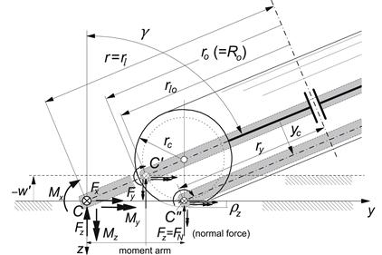
FIGURE 4.27 The motorcycle wheel at very large camber angle γ. Two alternative approaches to define the contact center C and the associated ‘loaded radius’ rl and as a consequence the overturning couple Mx. Instead of the circle, the actual section contour may be taken.
Although still perfectly correct, this standard definition may seem less attractive and one might want to choose for an alternative approach. Two possible alternatives have been indicated in Figure 4.27. The first one employs a value for the loaded radius ![]() that remains equal to the value that holds for the upright wheel: rlo which is equal to the free radius ro minus the normal deflection ρz. It should then be realized that a concurrent (slight) rise −w′ of the effective road plane (cf. Chap.10) may not be negligible. This method to acquire the overturning couple
that remains equal to the value that holds for the upright wheel: rlo which is equal to the free radius ro minus the normal deflection ρz. It should then be realized that a concurrent (slight) rise −w′ of the effective road plane (cf. Chap.10) may not be negligible. This method to acquire the overturning couple ![]() corresponds to the practical procedure often employed when measuring on the road where the actual height of the wheel center above the road surface is not measured. The second alternative is possibly the physically most realistic one. It defines a contact center located C″ above the lowest point of the undeformed tire. A drawback is that an effective wheel plane has to be defined in the vehicle dynamic model that is shifted with respect to the wheel center plane over a distance yc.
corresponds to the practical procedure often employed when measuring on the road where the actual height of the wheel center above the road surface is not measured. The second alternative is possibly the physically most realistic one. It defines a contact center located C″ above the lowest point of the undeformed tire. A drawback is that an effective wheel plane has to be defined in the vehicle dynamic model that is shifted with respect to the wheel center plane over a distance yc.
It turns out that the overturning couples that would act about the three possible virtual contact centers, defined above, become quite different from each other although the moment about the longitudinal axis through the wheel center remains, of course, the same. We find successively if the resultant normal force is assumed to act along a line that passes through the lowest point of the (supposedly circular) tire cross section and a through Fy with lateral compliance induced additional shift is disregarded:
1. Standard definition, using C (for general contour and for circular section):
![]() (4.125)
(4.125)
![]() (4.126)
(4.126)
2. Practical definition, using C′
![]() (4.127)
(4.127)
![]() (4.128)
(4.128)
![]() (4.129)
(4.129)
3. Physically more realistic definition, using C″
![]() (4.130)
(4.130)
![]() (4.131)
(4.131)
![]() (4.132)
(4.132)
The forces act in the points C, C′, and C″, respectively.
The overturning couple Mx according to the standard definition (4.126) is directly responsible for the lean angle of the motorcycle in a steady turn to become larger than what would be expected according to the ratio of centrifugal force and vehicle weight. In the practical definition, it would be the combination of ![]() and the effective road surface rise w′ that causes the increase in roll angle, while with the third definition it would be due to the lateral shift yc of the virtual wheel plane.
and the effective road surface rise w′ that causes the increase in roll angle, while with the third definition it would be due to the lateral shift yc of the virtual wheel plane.
Irrespective of the definition employed, it must be clear how the measured data have been processed and converted from the wheel axle system of axes (where in general the forces are measured) to the road and line of intersection-based axes system. An additional conversion may be necessary to suit the requirements of the vehicle dynamicist. It may be realized that with respect to the standard definition of the loaded radius rl, Eqn (4.125), the effective rolling radius re follows a quite different course. Also at large camber angles, re will remain close to the radius ![]() defined by (4.130) and shown in Figure 4.27.
defined by (4.130) and shown in Figure 4.27.
To account for the effect of the lateral tire deflection and through that the change in vertical pressure distribution, the part of Mx attributed to wheel camber and defined by one of the above or similar expressions should be extended with the part of the overturning couple described by Eqns (4.122–4.124) or, if appropriate, by a simpler version of that.
Note on the Aligning Torque at Large Camber
It may be of interest to be aware of another unexpected phenomenon that arises at large camber angles. One might make a mistake when deriving the aligning torque from the wheel axle-oriented measured forces and moments. If these latter quantities are denoted with an additional subscript a, the aligning torque is obtained from the moment equilibrium about the vertical axis as follows (cf. Figure 4.27):
![]() (4.133)
(4.133)
or alternatively from the moment equilibrium about the wheel radius:
![]() (4.134)
(4.134)
If the fact is not recognized that at camber a longitudinal force Fx is generated even at free rolling where Mya is zero or very small, and consequently, Fxa is disregarded in Eqn (4.133), the calculated aligning torque is incorrect. For a freely rolling tire with ![]() , the longitudinal force appears to read
, the longitudinal force appears to read
![]() (4.135)
(4.135)
4.3.6 Comparison with Experimental Data for a Car, a Truck, and a Motorcycle Tire
In Figures 4.28, 4.29 and 4.31, 4.32, the computed and measured characteristics of a 195/65 R15 car tire (on the road with Delft Tire Test Trailer, averaged over two slip angle and brake pressure sweep cycles) and of a 315/80 R22.5 truck tire (on Calspan flat track test stand) have been presented. Test and model results of a 180/55ZR17 motorcycle tire have been presented in Figures 11.33, 11.34. This tire has been tested with the TNO Tire Test-Semi-Trailer, cf. Figure 12.1 (replacement of the Delft Tire Test Trailer but equipped with the same measuring stations) using the new specially developed test device that can handle large camber angles (up to 70 degrees), cf. Figure 12.2. The fitted results have been obtained using the newly adapted Magic Formula model that is now suitable for fitting data for large camber angles as well, cf. Section 4.3.2.
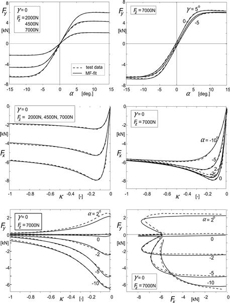
FIGURE 4.28 Force characteristics of a 195/65 R15 car tire. Magic Formula computed results compared with data from measurements (dotted curves) conducted with the Delft Tire Test Trailer (2000).
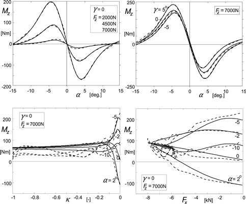
FIGURE 4.29 Aligning torque characteristics of a 195/65 R15 car tire. Magic Formula model-computed results compared with data from measurements (dotted curves) conducted with the Delft Tire Test Trailer (2000).
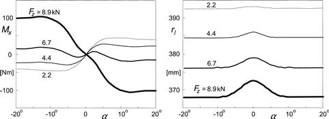
FIGURE 4.30 Overturning couple and loaded radius of a passenger car tire measured on Ford’s MTS Flat-Trac III tire testing machine (V.d. Jagt 2000). Compare with Figure 4.26.
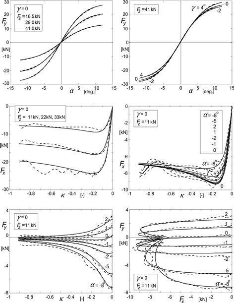
FIGURE 4.31 Force characteristics of a 315/80 R22.5 truck tire. Magic Formula-computed results compared with data from measurements conducted with the Calspan flat track tire test facility (2000) (dotted curves).
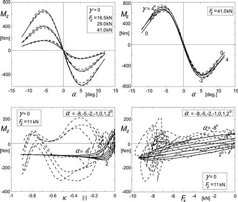
FIGURE 4.32 Aligning torque characteristics of a 315/80 R22.5 truck tire. Magic Formula-computed results compared with data from measurements conducted with the Calspan flat track tire test facility (2000) (dotted curves).
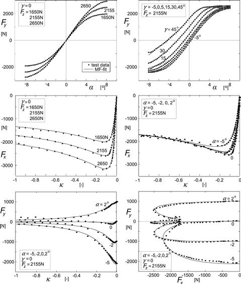
FIGURE 4.33 Force characteristics of a 180/55ZR17 motorcycle tire. Magic Formula-computed results compared with data from measurements conducted with the TNO test-semi-trailer, equipped with large camber test device (cf. Figure 12.2).
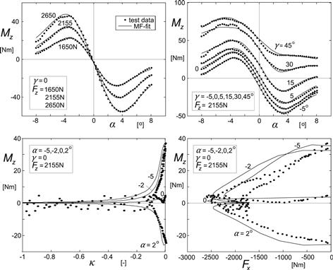
FIGURE 4.34 Aligning torque characteristics of a 180/55ZR17 motorcycle tire. Magic Formula-computed results compared with data from measurements conducted with the TNO test-semi-trailer, equipped with large camber test device (cf. Figure 12.2).
In general, it is observed that good agreement between computed and measured curves can be achieved with the model. An exception is the attempt to (physically) describe the measured course of the aligning torque at braking (except for the motorcycle tire). The diagrams concerned, in Figures 4.29 and 4.32, show a rather unpredictable variation of the moment while the brake pressure is increased until wheel lock is reached. This is supposedly due to the large direct contribution of the braking force times the moment arm. This distance between the line of action of Fx and the wheel center plane is suspected to vary due to local road camber variations and possibly tire nonuniformities while the tire rolls. Apparently, the motorcycle tire with narrow contact patch is much less sensitive to this effect.
Figure 4.30 presents the overturning couple and the loaded radius for a passenger car tire as reported by Van der Jagt (2000) and measured with the Ford MTS Flat-Trac III tire testing facility (cf. Figure 12.3). One may compare the measured characteristics with the calculated curves shown in Figure 4.26 obtained from Eqns (4.122–4.124) with hypothetical (not optimized) parameter values (Table 4.3).
Exercise 4.1 Assessment of Off-Nominal Tire Side Force Characteristics and Combined Slip Characteristics with Fx as Input Quantity
Consider the diagrams of Figure 4.35. For the original (nominal) side force characteristic Fyo(α) and for the cornering stiffness vs wheel load characteristic CFα(Fz), employ the formulas as given by Eqns (4.6–4.9) using the data indicated in the figure. The variation of camber stiffness with wheel load CFγ(Fz) is assumed to be linear. To cover the combined slip situation, use Eqns (4.41–4.44) (note: CFα is expressed in N/degree, convert this first into N/rad to get in line with Eqn (4.42)). In Eqn (4.42a), choose n = 4. In the nominal condition, we have parameter values:
![]()
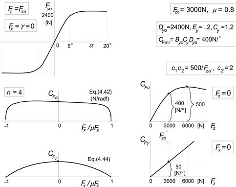
FIGURE 4.35 On the assessment of off-nominal and combined slip tire side force characteristics with longitudinal force as input quantity using the similarity method (Exercise 4.1).
Use Eqns (4.45, 4.46) and do the following:
1. Derive and plot the function Fy(α) for the following parameter values describing the tire at a different condition:
![]()
Exercise 4.2. Assessment of Force and Moment Characteristics at Pure and Combined Slip using the Magic Formula and the Similarity Method with κ as Input
Given are the pure slip force and moment characteristics at nominal vertical load Fzo = 4000 N and the cornering stiffness vs vertical load (cf. Figures 4.36, 4.37). The problems are formulated as follows:
1. Determine for the original curves, that is: at the nominal load, the values of the coefficients B, C, D, and E from the data indicated in the figures below. The vertical and horizontal shifts are disregarded. Use formula (4.49) for the longitudinal force, the side force, and also for the moment. Consider Figure 4.9 and use formulas (4.52, 4.53) and (4.56). Draw the resulting curves.
| μxo = 1.1 | μy0 = 1.0 |
| Fx,peak = 4400 N | Fy,peak = 4000 N |
| Fxa = 3400 N | Fya = 3400 N |
| κm = 0.07 | tan αm = 0.15 |
| CFκo = CFκ(4000) | CFα0 = CFα(4000) |
| p1 = 110 kN/rad | −Mz,peak = 100 Nm |
| p2 = 8000 N | −Mza= −20 Nm |
| further: | tan αm = 0.07 |
| CFκ(Fz) = 40Fz [N] | CMαo = CMα(4000) |
| effective compliance parameter | t(Fz) = 0.5 × 10⁻⁵Fz [m] |
| for Mz, Eqn (4.39): | CMα(Fz) = t.CFα(Fz) [Nm/rad] |
| c9 = 2 × 10⁻⁵Fzo/ao | c10 = 0 |
2. For Fz = 2000, 4000, and 6000 N with μx = μxo and μy = μyo while γ = 0, compute and plot the curves for pure slip Fx(κ), Fy(α) and Mz(α). Employ the similarity Eqns (4.21–4.26).
3. For Fz = 6000 N with μx = μxo, μy = μyo, and γ = 0 compute and plot the combined slip curves Fy(Fx) and Mz(Fx) at two slip angles: α = 2° and 8°. The values of the longitudinal slip may range from κ = −1 to +1. Use Eqns (4.27–4.29) and (4.35–4.40).
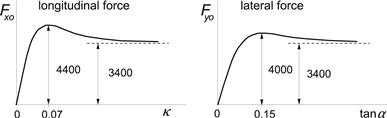
FIGURE 4.36 Original tire force characteristics at pure slip (Exercise 4.2).
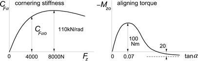
FIGURE 4.37 Cornering stiffness and original moment characteristics (Exercise 4.2).