Chapter 2
Basic Tire Modeling Considerations
Chapter Outline
2.2. Definition of Tire Input Quantities
2.3. Assessment of Tire Input Motion Components
2.4. Fundamental Differential Equations for a Rolling and Slipping Body
2.1 Introduction
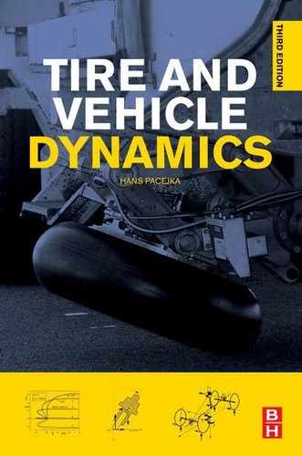
The performance of a tire as a force- and moment-generating structure is a result of a combination of several aspects. Factors that concern the primary tasks of the tire may be distinguished from factors that involve (often-important) secondary effects.
In Table 2.1 these factors are presented in matrix form. A further distinction is made between (quasi) steady state and vibratory behavior and, additionally, between symmetric (or in-plane) and anti-symmetric (or out-of-plane) aspects. The primary task factors appear in bold letters. The remaining factors are considered secondary factors.
TABLE 2.1 Tire Factors
The primary requirements to transmit forces in the three perpendicular directions (Fx, Fy, and Fz) and to cushion the vehicle against road irregularities involve secondary factors such as lateral and longitudinal distortions and slip. Although regarded as secondary phenomena, some of the quantities involved are crucial for the generation of the deformations and the associated forces and will be treated as input variables into the system.
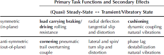
Figure 2.1 presents the ‘vectors’ of input and output components. In this diagram, the tire is assumed to be uniform and to move over a flat road surface. The input vector stems from motions of the wheel relative to the road. A precise definition of these input quantities is given in the next section.
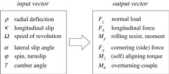
FIGURE 2.1 Input/output quantities (road surface considered flat).
For small deviations from the straight-ahead motion a linear description of behavior may be given. Then, it is advantageous to recognize the fact that the responses to the symmetric and anti-symmetric motions of the assumedly symmetric wheel–tire system can be considered as uncoupled. Figure 2.2 shows the separate function blocks with the input and output quantities. Here we have also considered the possibility of input from variations in road surface geometry and from tire nonuniformities resulting in e.g., out-of-roundness, stiffness variations, and ‘built-in’ forces.
FIGURE 2.2 Wheel axle motion and road surface coordinates and possibly uncoupled tire system blocks valid for small deviations from the steady-state straight ahead motion.
The forces and moments are considered as output quantities. It is sometimes beneficial to assume these forces to act on a rigid disk with inertial properties equal to those of the tire when considered rigid. These forces may differ from the forces acting between the road and the tire because of the dynamic forces acting on the tire when vibrating relative to the wheel rim. The motions of the wheel rim and the profile of the road, represented by its height w and its forward and transverse slope at or near the contact center, are regarded as input quantities to the tire. Braking and driving torques Ma are considered to act on the rotating wheel inertia Iw. For the freely rolling tire (then, by definition Ma = 0), the wheel angular motion about the spindle axis is governed by only the internal moment Mη acting between the rim and the tire. The five motion components of the wheel-spin axis may then remain to serve as input vector.
The discussion on the force generation and dynamic properties of the tire will be conducted along the two main lines: symmetric and anti-symmetric behavior. Interaction between these main groups of input motions complicates the situation (combined slip). These interactions become important if at least one of the input motions or more precisely, one of the associated slip components becomes relatively large. Because of its relative simplicity, steady-state behavior will be treated first (Chapter 3). The discussion on tire dynamic behavior starts in Chapter 5.
2.2 Definition of Tire Input Quantities
If the problem that is going to be investigated involves road irregularities, then the location and the orientation of the stub axle (spindle axis) must be known with respect to the specific irregularity met on the road. The road surface is defined with respect to a coordinate system of axes attached to the road. If the position and orientation of the axle are known with respect to the fixed triad, then the exact position of the wheel with respect to the possibly irregular road surface can be determined. This relative position and orientation of the wheel with respect to the road are important to derive the radial tire deflection and the relative attitude (camber) and to assess the current value of the friction coefficient, which may vary due to e.g., slippery spots or nonhomogeneous surface conditions (grooves). The time rate of change of this relative position is needed not only for possible hysteresis effects but also mainly for the determination of the so-called ‘slip’ of the wheel with respect to the ground.
If the road surface near the contact patch can be approximated by a flat plane (that is, when the smallest considered wavelength of the decomposed surface vertical profile is large with respect to the contact length and its amplitude small), the distance of the wheel center to the road plane and the angle between wheel plane and the normal to the road surface will suffice in addition to the several slip quantities and the running speed of the wheel.
For the definition of the various motion and position input quantities listed in Figure 2.1, it is helpful to consider Figure 2.3. A number of planes have been drawn. The road plane and the wheel-center plane (with line of intersection along the unit vector l) and two planes normal to the road plane, one of which contains the vector l and the other the unit vector s, which is defined along the wheel-spin axis. From the figure follows the definition of the contact center C, also designated as the point of intersection (of the three planes). The unit vector t lies in the road plane and is directed perpendicular to l. The vector r forms the connection between wheel center A and the contact center C. Its length, r, is defined as the loaded radius of the tire. The position and attitude of the wheel with respect to the inertial triad are completely described by the vectors b + a and s. The road plane is defined at the contact center by the position vector of that point c and the normal to the road in that point represented by the unit vector n (positive upward). Figure 2.3 also shows two systems of axes (besides the inertial triad). First, we have introduced the road contact axes system (C, x, y, and z) of which the x-axis points forward along the line of intersection (l), the z-axis points downward normal to the road plane (–n), and the y-axis points to the right along the transverse unit vector t. Second, the wheel axle system of axes (A, ξ;, η, and ζ) has been defined with the ξ; axis parallel to the x-axis, the η axis along the wheel spindle axis (s), and the ζ axis along the radius (r).
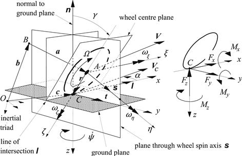
FIGURE 2.3 Definition of position, attitude, and motion of the wheel and the forces and moments acting from the road on the wheel. Directions shown are defined as positive.
Sign conventions in the literature are not uniform. For the sake of convenience and to reduce sources of making errors, we have chosen a sign convention that avoids working with negative quantities as much as possible.
The radial deflection of the tire ρ is defined as the reduction of the tire radius from the unloaded situation rf to the loaded case r:
![]() (2.1)
(2.1)
For positive ρ the wheel load Fz (positive upward) is positive as well.
The tangential or longitudinal slip κ requires deeper analysis. For the sake of properly defining the longitudinal slip, the so-called slip point S is introduced. This point is thought to be attached to the rim or wheel body at a radius equal to the slip radius rs and forms the center of rotation when the wheel rolls at a longitudinal slip equal to zero. The slip radius is the radius of the slip circle. At vanishing longitudinal slip, this slip circle rolls purely over an imaginary surface parallel to the road plane. The length of the slip radius depends on the definition of longitudinal slip that is adopted. A straightforward definition would be to make the slip radius equal to the loaded wheel radius. This, however, would already lead to a considerable magnitude of the longitudinal force Fx that would be generated at longitudinal slip equal to zero. A more convenient and physically proper definition corresponds to the situation that Fx = 0 at zero longitudinal slip. Because of the occurrence of rolling resistance, measurements of tire characteristics would then require the application of a driving torque to reach the condition of slip equal to zero! This may become of importance, especially when experiments are conducted at large camber angles where the drag may become considerable (motorcycle tires). An alternative, often-used definition takes the effective rolling radius re defined at free rolling (Ma = 0) as the slip radius. Under normal conditions, the resulting Fx vs κ diagrams according to the latter two definitions are very close. A small horizontal shift of the curves is sufficiently accurate to change from one definition to the other. The drawback of the last definition is that when testing on very low friction (icy) surfaces, the rolling resistance may be too large to let the wheel rotate without the application of a driving torque. Consequently, the state of free rolling cannot be realized under these conditions. Nevertheless, we will adopt the last definition where rs = re and consequently, point S is located at a distance re from the wheel center. Figure 2.4 depicts this configuration.
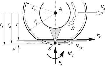
FIGURE 2.4 Effective rolling radius and longitudinal slip velocity.
According to this definition we will have the situation that when a wheel rolls freely (that is, at Ma = 0) at constant speed over a flat even road surface, the longitudinal slip κ is equal to zero. This notwithstanding the fact that at free rolling some fore and aft deformations will occur because of the presence of hysteresis in the tire that generates a rolling resistance moment My. Through this a rolling resistance force Fr = My /r arises, which necessarily is accompanied by tangential deformations. We may agree that at the instant of observation, point S, which lies on the slip circle and is attached to the wheel rim, has reached its lowest position, that is: on the line along the radius vector r. At free rolling, its velocity has then become equal to zero and point S has become the center of rotation of the motion of the wheel rim. We have at free rolling on a flat road for a wheel in upright position (γ = 0) and/or without wheel yaw rate ![]() , cf. Figure 2.3, a velocity of the wheel center in the forward (x or ξ;) direction:
, cf. Figure 2.3, a velocity of the wheel center in the forward (x or ξ;) direction:
![]() (2.2)
(2.2)
with Ω denoting the speed of revolution of the wheel body to be defined hereafter. By using this relationship, the value of the effective rolling radius can be assessed from an experiment. The forward speed and the wheel speed of revolution are both measured while the wheel axle is moved along a straight line over a flat road. Division of both quantities leads to the value of re. The effective rolling radius will be a function of the normal load and the speed of travel. We may possibly have to take into account the dependency on the camber angle and the slip angle.
If at braking or driving the longitudinal slip is no longer zero, point S will move with a longitudinal slip speed Vsx that differs from zero. We obviously obtain if again ![]() :
:
![]() (2.3)
(2.3)
The longitudinal slip (sometimes called the slip ratio) is denoted by κ and may be tentatively defined as the ratio of longitudinal slip velocity −Vsx of point S and the forward speed of the wheel center Vx:
![]() (2.4)
(2.4)
or with (2.3):
![]() (2.5)
(2.5)
This again holds for a wheel on a flat road and with ![]() . A more general and precise definition of κ will be given later on. The sign of the longitudinal slip κ has been chosen such that at driving, when Fx > 0, κ is positive and at braking, when Fx < 0, κ is negative. When the wheel is locked (Ω = 0), we obviously have κ = –1. In the literature, the symbol s (or S) is more commonly used to denote the slip ratio.
. A more general and precise definition of κ will be given later on. The sign of the longitudinal slip κ has been chosen such that at driving, when Fx > 0, κ is positive and at braking, when Fx < 0, κ is negative. When the wheel is locked (Ω = 0), we obviously have κ = –1. In the literature, the symbol s (or S) is more commonly used to denote the slip ratio.
The angular speed of rolling Ωr, more precisely defined for the case of moving over undulated road surfaces, is the time rate of change of the angle between the radius connecting S and A (this radius is thought to be attached to the wheel) and the radius r defined in Figure 2.3 (always lying in the plane normal to the road through the wheel-spin axis). Figure 2.5 illustrates the situation.
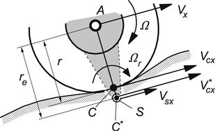
FIGURE 2.5 Rolling and slipping of a tire over an undulated road surface.
The linear speed of rolling Vr is defined as the velocity with which an imaginary point C∗, which is positioned on the line along the radius vector r and coincides with point S at the instant of observation, moves forward (in x direction) with respect to point S that is fixed to the wheel rim:
![]() (2.6)
(2.6)
For a tire freely rolling over a flat road we have, Ωr = Ω and with ![]() in addition: Vr = Vx. Note, that at wheel lock (Ω = 0) the angular speed of rolling Ωr is not equal to zero when the wheel moves over a road with a curved vertical profile (then not always the same point of the wheel is in contact with the road). For a cambered wheel showing a yaw rate
in addition: Vr = Vx. Note, that at wheel lock (Ω = 0) the angular speed of rolling Ωr is not equal to zero when the wheel moves over a road with a curved vertical profile (then not always the same point of the wheel is in contact with the road). For a cambered wheel showing a yaw rate ![]() , pure rolling can occur on a flat road even when the speed of the wheel center Vx = 0. In that case a linear speed of rolling arises that is equal to Vr = re
, pure rolling can occur on a flat road even when the speed of the wheel center Vx = 0. In that case a linear speed of rolling arises that is equal to Vr = re![]() sin γ and consequently an angular speed of rolling Ωr =
sin γ and consequently an angular speed of rolling Ωr = ![]() sin γ.
sin γ.
In the normal case of an approximately horizontal road surface, the wheel speed of revolution Ω may be defined as the angular speed of the wheel body (rim) seen with respect to a vertical plane that passes through the wheel spindle axis. On a flat level road, the angular speed of rolling Ωr and the speed of revolution of the wheel Ω are equal to each other. The absolute speed of rotation of the wheel about the spindle axis ωη will be different from –Ω when the wheel is cambered and a yaw rate about the normal to the road occurs of the plane that passes through the spindle axis and is oriented normal to the road. Then (cf. Figure 2.6):
![]() (2.7)
(2.7)
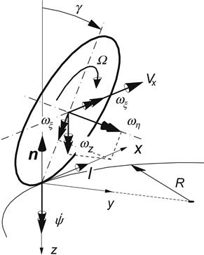
FIGURE 2.6 Rotational slip resulting from path curvature and wheel camber (slip angle = 0).
This equation forms a correct basis for a general definition of Ω also on nonlevel road surfaces. Its computation is straightforward if ωη is available from wheel dynamics calculations.
The longitudinal running speed ![]() is defined as the longitudinal component of the velocity of propagation of the imaginary point C∗ (on radius vector r) in the direction of the x-axis (vector l). In case the wheel is moved in such a way that the same point remains in contact with the road, we would have
is defined as the longitudinal component of the velocity of propagation of the imaginary point C∗ (on radius vector r) in the direction of the x-axis (vector l). In case the wheel is moved in such a way that the same point remains in contact with the road, we would have ![]() . This corresponds to wheel lock when the road is flat and the vehicle pitch rate is zero. For a freely rolling tire the longitudinal running speed equals the linear speed of rolling:
. This corresponds to wheel lock when the road is flat and the vehicle pitch rate is zero. For a freely rolling tire the longitudinal running speed equals the linear speed of rolling: ![]() . On a flat road and at zero camber or zero yaw rate
. On a flat road and at zero camber or zero yaw rate ![]() , we obtain
, we obtain ![]() . The general definition for longitudinal slip now reads:
. The general definition for longitudinal slip now reads:
![]() (2.8)
(2.8)
The lateral slip is defined as the ratio of the lateral velocity ![]() of the contact center C and the longitudinal running speed
of the contact center C and the longitudinal running speed ![]() . We have in terms of the slip angle α:
. We have in terms of the slip angle α:
![]() (2.9)
(2.9)
which for a wheel, not showing camber rate ![]() nor radial deflection rate
nor radial deflection rate ![]() and yaw rate
and yaw rate ![]() at nonzero camber angle γ, when running on a flat road reduces to the ratio of lateral and forward speed of the wheel center:
at nonzero camber angle γ, when running on a flat road reduces to the ratio of lateral and forward speed of the wheel center:
![]() (2.10)
(2.10)
In practice, points C and C∗ lie close together and making a distinction between the longitudinal or the lateral velocities of these points is only of academic interest and may be neglected. Instead of ![]() in the denominator, we may write
in the denominator, we may write ![]() and if we wish, instead of
and if we wish, instead of ![]() in the numerator the lateral speed of point S (parallel to road plane), which is
in the numerator the lateral speed of point S (parallel to road plane), which is ![]() . The definitions of the slip components then reduce to
. The definitions of the slip components then reduce to
![]() (2.11)
(2.11)
![]() (2.12)
(2.12)
The slip velocities ![]() and
and ![]() form the components of the slip speed vector
form the components of the slip speed vector ![]() and κ and tan α the components of the slip vector ss. We have
and κ and tan α the components of the slip vector ss. We have
![]() (2.13)
(2.13)
and
![]() (2.14)
(2.14)
The ‘spin’ slip φ is defined as the component −ωz of the absolute speed of rotation vector ω of the wheel body along the normal to the road plane n divided by the speed of C. We obtain the expression in terms of yaw rate ![]() and camber angle γ (cf. Figure 2.6):
and camber angle γ (cf. Figure 2.6):
![]() (2.15)
(2.15)
The minus sign is introduced again to remain consistent with the definitions of longitudinal and lateral slip (2.11, 2.12). Then, we will have as a result of a positive φ a positive moment Mz. It turns out that then also the resulting side force Fy is positive. The yaw rate ![]() is defined as the speed of rotation of the line of intersection (unit vector l) about the z-axis normal to the road cf. Figure 2.3. If the side slip angle remains constant
is defined as the speed of rotation of the line of intersection (unit vector l) about the z-axis normal to the road cf. Figure 2.3. If the side slip angle remains constant ![]() and the wheel moves over a flat road, Eqn (2.15) may be written as
and the wheel moves over a flat road, Eqn (2.15) may be written as
![]() (2.16)
(2.16)
When the tire rolls freely (then Vsx = 0, Vc = Vr), we obviously obtain
![]() (2.17)
(2.17)
with 1/R denoting the momentary curvature of the path of C∗ or approximately of the contact center C.
For a tire we shall distinguish between spin due to path curvature and spin due to wheel camber. For a homogeneous ball, the effect of both input quantities is the same. For further use, we define turn slip as
![]() (2.18)
(2.18)
Wheel camber or wheel inclination angle γ is defined as the angle between the wheel-center plane and the normal to the road. With Figure 2.3 we find
![]() (2.19)
(2.19)
or on flat level roads:
![]() (2.20)
(2.20)
where sz represents the vertical component of the unit vector s along the wheel-spin axis.
2.3 Assessment of Tire Input Motion Components
The location of the contact center C and the magnitude of the wheel radius r result from the road geometry and the position of the wheel axle. We consider the approximate assumption that the road plane is defined by the plane touching the surface at point Q located vertically below the wheel center A. The position of point Q with respect to the inertial frame (Oo, xo, yo, zo) is given by vector q. The normal to the road plane is defined by unit vector n. The location of a reference point B of the vehicle is defined by vector b and the location of the wheel center A by b + a (cf. Figure 2.3). The orientation of the wheel-spin axis is given by unit vector s and the location of the contact center C by
![]() (2.21)
(2.21)
where r is still to be determined. The expression for r is derived from the equations:
![]() (2.22)
(2.22)
with
![]() (2.23)
(2.23)
(with λ resulting from the condition that |l|= 1) and with (2.21) in order to obtain the magnitude of the loaded radius r:
![]() (2.24)
(2.24)
which indicates that contact point C and road point Q lie on the same plane perpendicular to n. On flat level roads, the above equations become a lot simpler since in that case nT = (0, 0, −1) and the z components of c and q become zero.
For small camber the radial tire deflection ρ is now readily obtained from (cf. Figure 4.27 and Eqn (7.46) for the deflection normal to the road):
![]() (2.25)
(2.25)
with rf the free unloaded radius. For a given tire the effective rolling radius re is a function of among other things the unloaded radius, the radial deflection, the camber angle, and the speed of travel.
The vector for the speed of propagation of the contact center Vc representing the magnitude and direction of the velocity with which point C moves over the road surface is obtained by differentiation with respect to time of position vector c (2.21):
![]() (2.26)
(2.26)
with V the velocity vector of the wheel center A (Figure 2.3). The speed of propagation of point C∗ represented by vector ![]() becomes (cf. Figure 2.5 and assume re/r constant):
becomes (cf. Figure 2.5 and assume re/r constant):
![]() (2.27)
(2.27)
The velocity vector of point S that is fixed to the wheel body results from
![]() (2.28)
(2.28)
with ω being the angular velocity vector of the wheel body with respect to the inertial frame. On the other hand, this velocity is equal to the speed of point C∗ minus the linear speed of rolling:
![]() (2.29)
(2.29)
![]() (2.30)
(2.30)
or
![]() (2.31)
(2.31)
The linear speed of rolling is, according to (2.6), related to the angular speed of rolling:
![]() (2.32)
(2.32)
Of course, on flat roads Ωr = Ω, which is the wheel speed of revolution and may be directly calculated by using the relationship (2.7).
The lateral slip speed Vcy is obtained by taking the lateral component of Vc(2.26):
![]() (2.33)
(2.33)
with
![]() (2.34)
(2.34)
The lateral slip tan α reads
![]() (2.35)
(2.35)
The longitudinal slip speed Vsx is obtained in a similar way:
![]() (2.36)
(2.36)
The longitudinal slip κ now becomes
![]() (2.37)
(2.37)
The turn slip according to definition (2.18) is derived as follows:
![]() (2.38)
(2.38)
with the time derivative of the unit vector l in the numerator. The wheel camber angle is obtained as indicated before:
![]() (2.39)
(2.39)
Exercise 2.1 Slip and Rolling Speed of a Wheel Steered About a Vertical Axis
The vehicle depicted in Figure 2.7 runs over a flat level road. The rear frame moves with velocities u, v, and r with respect to an inertial triad (choose (Oo, xo, yo, zo) that at the instant considered is positioned parallel to the moving triad (B, x, y, z) attached to the rear frame). The front frame can be turned with a rate ![]() (= dδ /dt) with respect to the rear frame. At the instant considered, the front frame is steered over an angle δ.
(= dδ /dt) with respect to the rear frame. At the instant considered, the front frame is steered over an angle δ.
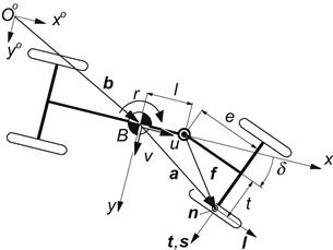
FIGURE 2.7 Top view of vehicle (Exercise 2.1).
It is assumed that the effective rolling radius is equal to the loaded radius (re = r, C∗ = C ). The longitudinal slip at the front wheels is assumed to be equal to zero (Vsx = 0).
Derive expressions for the lateral slip speed Vcy, the linear speed of rolling Vr, and the lateral slip tanα for the right front wheel.
Exercise 2.2 Slip and Rolling Speed of a Wheel Steered About an Inclined Axis (Motorcycle)
The wheel shown in Figure 2.8 runs over a flat level road surface. Its center A moves along a horizontal straight line at a height H with a speed u. The rake angle ε is 45°. The steer axis BA (vector a) translates with the same speed u. There is no wheel slip in the longitudinal direction (Vsx = 0). Again we assume re = r. For the sake of simplifying this complex problem, it is assumed that the wheel center height H is a given constant.
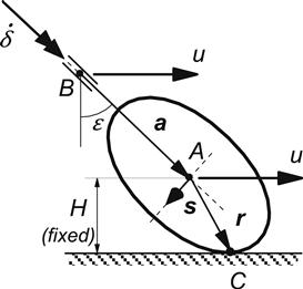
FIGURE 2.8 Side view of the front part of vehicle (motorcycle) with wheel turned over angle δ about steer axis (a) (Exercise 2.2).
Derive expressions for the lateral slip speed Vcy, the linear speed of rolling Vr, and the turn slip speed ![]() in terms of H, u, and
in terms of H, u, and ![]() for δ = 0°, 30°, and 90°. Also show the expressions for the slip angle α, the camber angle γ, and the spin slip φ with contributions both from turning and camber. Note that in reality height H depends on δ and changes with
for δ = 0°, 30°, and 90°. Also show the expressions for the slip angle α, the camber angle γ, and the spin slip φ with contributions both from turning and camber. Note that in reality height H depends on δ and changes with ![]() .
.
2.4 Fundamental Differential Equations for a Rolling and Slipping Body
A wheel with tire that rolls over a smooth level surface and at the same time performs longitudinal and lateral slipping motions will develop horizontal deformations as a result of the presence of frictional forces that attempt to prevent the tire particles, which have entered the contact area, from sliding over the road. Besides areas of adhesion, areas of sliding may occur in the contact patch. The latter condition will arise when the deflection generated in the range of adhesion would have become too large to be maintained by the available frictional forces. In the following, a set of partial differential equations will be derived that governs the horizontal tire deflections in the contact area in connection with possibly occurring velocities of sliding of the tire particles. For a given physical structure of the tire, these equations can be used to develop the complete mathematical description of tire model behavior as will be demonstrated in subsequent chapters.
Consider a rotationally symmetric elastic body representing a wheel and tire rolling over a smooth horizontal rigid surface representing the road. As indicated in Figure 2.9 a system of axes (Oo, xo, yo, zo) is assumed to be fixed to the road. The xo and yo axes lie in the road surface and the zo axis points downward. Another coordinate system (C, x, y, z) is introduced of which the axes x and y lie in the (xo, Oo, yo) plane and z points downward. The x-axis is defined to lie in the wheel center plane and the y-axis forms the vertical projection of the wheel spindle axis. The origin C, which is the so-called contact center or, perhaps better: the point of intersection, travels with an assumedly constant speed Vc over the (xo, Oo, yo) plane. The traveled distance s is
![]() (2.40)
(2.40)
where t denotes the time. The tangent to the orbit of C makes an angle β with the fixed xo-axis. With respect to this tangent, the x-axis is rotated over an angle α, defined as the slip angle. The angular deviation of the x-axis with respect to the xo-axis (that is the yaw angle) becomes
![]() (2.41)
(2.41)
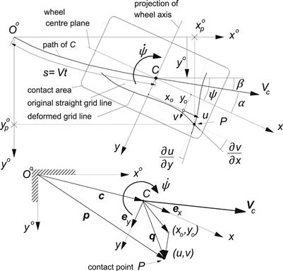
FIGURE 2.9 Top view of tire contact area showing its position with respect to the system of axes (Oo, xo, yo, zo) fixed to the road and its deformations (u, v) with respect to the moving triad (C, x, y, z).
For angle β the following relation with yo, the lateral displacement of C, holds
![]() (2.42)
(2.42)
As a result of friction, horizontal deformations may occur in the contact patch. The corresponding displacements of a contact point with respect to the position this material point would have in the horizontally undisturbed state (defined to occur when rolling on a frictionless surface), with coordinates (xo, yo), are indicated by u and v in x and y directions, respectively. These displacements are functions of coordinates x and y and of the traveled distance s or the time t.
The position in space of a material point of the rolling and slipping body in contact with the road (cf. Figure 2.9) is indicated by the vector:
![]() (2.43)
(2.43)
where c indicates the position of the contact center C in space and q the position of the material point with respect to the contact center. We have for the latter vector
![]() (2.44)
(2.44)
with ex (= l) and ey (= t) representing the unit vectors in x and y directions. The vector of the sliding velocity of the material point relative to the road obviously becomes
![]() (2.45)
(2.45)
where ![]() denotes the vector of the speed of propagation of contact center C.
denotes the vector of the speed of propagation of contact center C.
The coordinates xo and yo of the material contact point of the horizontally undisturbed tire (zero friction) will change due to rolling. Then, the point will move through the contact area from the leading edge to the trailing edge. In the general case, e.g., of an elastic ball rolling over the ground, we may have rolling in both the forward and lateral directions. Then, both coordinates of the material point will change with time. In the present analysis of the rolling wheel, we will disregard the possibility of sideways rolling.
To assess the variation in the coordinates of the point on the zero friction surface, let us first consider an imaginary road surface that is in the same position as the actual surface but does not transmit forces to the wheel. Then, the tire penetrates the imaginary surface without deformation. When the general situation is considered of a wheel-spin axis that is inclined with respect to the imaginary road surface, i.e., rolling at a camber angle γ, the coordinates x and y of the material point change with time as follows:
 (2.46)
If ![]() , the effect of the time rate of change of the camber angle (wheel plane rotation about the x-axis) on the partial derivative ∂y/∂t and thus on
, the effect of the time rate of change of the camber angle (wheel plane rotation about the x-axis) on the partial derivative ∂y/∂t and thus on ![]() may be neglected. This effect is directly connected with the small instantaneous or so-called nonlagging response to camber changes. Similar instantaneous responses may occur as a result of normal load changes when the tire shows conicity or ply-steer. The terms associated with ∂y/∂t have been neglected in the above equation and related neglects will be performed in subsequent formulas for
may be neglected. This effect is directly connected with the small instantaneous or so-called nonlagging response to camber changes. Similar instantaneous responses may occur as a result of normal load changes when the tire shows conicity or ply-steer. The terms associated with ∂y/∂t have been neglected in the above equation and related neglects will be performed in subsequent formulas for ![]() .
.
The radius of the outer surface in the undeformed state ro may depend on the lateral coordinate y. If the rolling body shows a touching surface that is already parallel to the road before it is deformed, we would have in the neighborhood of the center of contact: ro(y) = ro(0) − y sin![]() γ. In case of a cambered car tire, a distortion of belt and carcass is needed to establish contact over a finite area with the ground. The shape of the tire cross section in the undeformed state governs the dependency of the free radius with the distance to the wheel center plane.
γ. In case of a cambered car tire, a distortion of belt and carcass is needed to establish contact over a finite area with the ground. The shape of the tire cross section in the undeformed state governs the dependency of the free radius with the distance to the wheel center plane.
In Figure 2.10, an example is given of two different cases. The upper part corresponds to a rear view and the lower one to a plan view of a motorcycle tire and of a car tire pressed against an assumedly frictionless surface (μ = 0). It may be noted that in case of a large camber angle like with the motorcycle tire, one might decide to redefine the position of the x- and z-axes. The contact line which is the part of the peripheral line that touches the road surface has been indicated in the figure.

FIGURE 2.10 A motorcycle tire (left) and a car tire (right) in cambered position touching the assumedly frictionless road surface. The former without and the latter with torsion and bending of the carcass and belt. Top: rear view; bottom: top view.
When the tire is loaded against an assumedly frictionless rigid surface, deformations of the tire will occur. These will be due to: (1) lateral and longitudinal compression in the contact region, (2) a possibly not quite symmetric structure of the tire resulting in effects known as ply-steer and conicity, and (3) loading at a camber angle that will result in distortion of the carcass and belt. The deformations occurring in the contact plane will be denoted as uo and vo. We will introduce the functions θx,y(x, y) representing the partial derivatives of these normal-load-induced longitudinal and lateral deformations with respect to x. We have
![]() (2.47)
(2.47)
These functions depend on the vertical load and on the camber angle.
If the tire is considered to roll on a frictionless flat surface at a camber angle or with nonzero θs, lateral and longitudinal sliding of the contact points will occur even when the wheel does not exhibit lateral, longitudinal, or turn slip. Since horizontal forces do not occur in this imaginary case, u and v are defined to be zero. The coordinates with respect to the moving axes system (C, x, y, z) of the contact point sliding over the hypothetical frictionless surface were denoted as xo and yo. The time rates of change of xo and yo depend on the position in the contact patch, on the speed of rolling Ω, and on the camber angle γ. We find after disregarding the effect of ∂yo/∂t:
 (2.48)
For homogeneous rolling bodies (e.g., a railway wheel or a rubber ball) with counter surfaces already parallel before touching, torsion about the longitudinal axis and lateral bending do not occur, ply-steer and conicity are absent, and horizontal compression may be neglected (θ’s vanish). Moreover, we then had: ro(y) = ro(0) – y sin γ so that for this special case (2.48) reduces to
![]() (2.49)
(2.49)
For a tire the terms with θ are appropriate. Circumferential compression (θx < 0) decreases the effective rolling radius re that is defined at free rolling. At camber, due to the structure of a car tire with a belt that is relatively stiff in lateral bending, the compression/extension factor θx will not be able to compensate for the fact that a car tire shows only a relatively small variation in the free radius ro(y) across the width of the tread, while for the same reason the lateral distortion factor θy appears to be capable of considerably counteracting the effect of the term with sinγ in the second Eqn (2.48). For a motorcycle tire with a cross section approximately forming a sector of a circle, touching at camber is accomplished practically without torsion about a longitudinal axis and the associated lateral bending of the tire near the contact zone. Figure 2.10 illustrates the expected deformations and the resulting much smaller curvature of the contact line on a frictionless surface for the car tire relative to the curvature exhibited by the motorcycle tire. Since on a surface with friction the rolling tire will be deformed to acquire a straight contact line, this observation may explain the relatively low camber stiffness of the car and truck tire.
As mentioned above, circumferential compression of belt and tread resulting from the normal loading process (somewhat counteracted by the presence of hysteresis also represented by the factor θx) gives rise to a decrease in the effective rolling radius. The compression may not be uniform along the x-axis. For our purposes, however, we will disregard the resulting secondary effects. The coefficient in (2.48) that relates passage velocity ![]() and speed of revolution Ω of the wheel is designated as local effective rolling radius rej at e.g., row j of tread elements. This radius depends on lateral position yj and will change with vertical load Fz and camber angle γ. The velocity through the contact zone of the elements of row j is:
and speed of revolution Ω of the wheel is designated as local effective rolling radius rej at e.g., row j of tread elements. This radius depends on lateral position yj and will change with vertical load Fz and camber angle γ. The velocity through the contact zone of the elements of row j is: ![]() . We may write
. We may write
![]() (2.50)
(2.50)
in which use has been made of the overall tire effective rolling radius re defined according to Eqns (2.2, 2.6) and Δrej(yj), the possibly anti-symmetric variation in the local effective rolling radius over the tread width with respect to re due to loading at camber or conicity. The (average) effective rolling radius re is expected to depend on the camber angle as well.
We will now try to make a distinction between the contributions to the anti-symmetric variation originating from conicity and from camber. We write for the local passage velocity:
![]() (2.51)
(2.51)
In this way, we have achieved a structure closely related to the first equation of (2.49). For a rolling elastic body such as a ball or a motorcycle tire, θγx will be (close to) zero, while a car, truck or racing car tire is expected to have a θγx closer to −1. A bias-ply tire featuring a more compliant carcass and tread band and a rounder cross-section profile is expected to better ‘recover’ from the torsion effects, resulting in a value in-between the two extremes. It is true that in general bias-ply tires show considerably larger side forces as a result of camber than radial ply car tires.
When the product of θy and ro − re is considered to be negligible, we write for the lateral velocity of the points over a frictionless surface with respect to the x-axis instead of (2.48):
![]() (2.52)
(2.52)
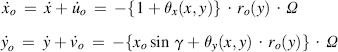
The resulting expressions (2.51, 2.52) may now be substituted in expression (2.45) for the sliding speed components.
For a given material point of the tire outer surface that now rolls on a road surface with friction reintroduced, the associated deflections u and v (which occur on top of the initial load induced deflections uo and vo) are functions of its location in the contact patch and of the time: u = u(xo, yo, t) and v = v(xo, yo, t). Hence, we have for the time rates of change:
 (2.53)
in which the expressions (2.51, 2.52) apply. If we disregard sideways rolling and neglect a possible small effect of the variation in yo that occurs at camber, conicity, or ply-steer, the second terms of the right-hand members disappear. The remaining expressions are substituted in (2.45).
According to Eqn (2.29), the linear speed of rolling and the velocity of the contact center are related through the slip speed. We have (when disregarding the generally very small difference between the velocities of C∗ and C) the vector relationship:
![]() (2.54)
(2.54)
After simplifying the equations by neglecting products of assumedly small quantities (i.e., deflections and input (slip) quantities) and using the expression for ωz, which is the absolute angular velocity of the wheel body about the z-axis as indicated in Eqn (2.15), components of sliding velocity become
![]() (2.55)
(2.55)
![]() (2.56)
(2.56)
With all θ’s omitted we would return to the basic case of e.g., a ball rolling and slipping over a flat rigid surface. In Chapter 3, a physical tire model is developed using the above equations. There, the θ’s are expressed in terms of the camber angle and of equivalent camber and slip angles γcon and αply to account for conicity and ply-steer (cf. (Eqns 3.108, 3.109)).
Let us now consider the special case of a freely rolling tire subjected to only small lateral slip and spin (![]() , with R the instantaneous radius of path curvature, and thus
, with R the instantaneous radius of path curvature, and thus ![]() ) and neglect effects of initial non-parallelity of touching surfaces as well as ‘built-in’ load- and camber-induced deformation effects (all θ’s = 0). We then have (approximately)
) and neglect effects of initial non-parallelity of touching surfaces as well as ‘built-in’ load- and camber-induced deformation effects (all θ’s = 0). We then have (approximately)
![]() (2.57)
(2.57)
Using the traveled distance s (2.40) instead of the time t as an independent variable, we obtain the following expressions for the sliding velocities of a contact point with coordinates (x, y) of a freely rolling tire at small lateral slip and spin:
![]() (2.58)
(2.58)
![]() (2.59)
(2.59)
In the contact area, regions of adhesion may occur as well as regions where sliding takes place. In the region of adhesion, the tire particles touching the road do not move and we have Vgx = Vgy = 0. In this part of the contact area, the frictional shear forces acting from road to tire on a unit area (with components denoted by qx and qy not to be confused with the components of the position vector (2.44) used earlier) do not exceed the maximum available frictional force per unit area. The maximum frictional shear stress is governed by coefficient of friction μ and normal contact pressure qz. In the adhesion region, Eqns (2.58, 2.59) reduce to
![]() (2.60)
(2.60)
![]() (2.61)
(2.61)
Furthermore, we have the condition:
![]() (2.62)
(2.62)
In the region of sliding, Eqns (2.58, 2.59) hold. If the deformation gradients were known, the velocity components Vgx and Vgy might be obtained from these equations. For the frictional stress vector, we obtain:
![]() (2.63)
(2.63)
with
![]() (2.64)
(2.64)
For the simpler case that only lateral slip occurs (φ = 0), the equations for the lateral deformations reduce to:
in the adhesion region:
![]() (2.65)
(2.65)
in the sliding region:
![]() (2.66)
(2.66)
The Eqns (2.55, 2.56) apply in general. Their solutions contain constants of integration that depend on the selected physical model description of the tire. Applications of the differential equations derived above will be demonstrated in subsequent chapters both for steady-state and non-steady-state conditions. In the case of steady-state motion of the wheel, the partial derivatives with respect to time t or traveled distance s become equal to zero (∂v/∂s = ∂u/∂s = 0). Then, the deformation gradients in the area of adhesion (Vg = 0) follow easily from the then ordinary differential equations. In the last simple case (2.66) we would obtain: dv/dx = −α, which means that the contact line is straight and runs parallel to the speed vector Vc.
Exercise 2.3 Partial Differential Equations with Longitudinal Slip Included
Establish the differential equations for the sliding velocities similar to the Eqns (2.58, 2.59) but now with longitudinal slip κ included (α and φ remain small). Note that in that case Vr ≠ Vc and that Vr may be expressed in terms of Vcx (≈Vc) and κ. Also, find the partial differential equations governing the deflections in the adhesion zone similar to the Eqns (2.60, 2.61).
2.5 Tire Models (Introductory Discussion)
Several types of mathematical models of the tire have been developed during the past half-century; each type for a specific purpose. Different levels of accuracy and complexity may be introduced in the various categories of utilization. This often involves entirely different ways of approach. Figure 2.11 roughly illustrates how the intensity of various consequences associated with different ways of attacking the problem tends to vary. From left to right the model is based less on full-scale tire experiments and more on the theory of the behavior of the physical structure of the tire. In the middle, the model will be simpler but possibly less accurate while at the far right the description becomes complex and less suitable for application in the simulation of vehicle motions and may be more appropriate for the analysis of detailed tire performance in relation to its construction.
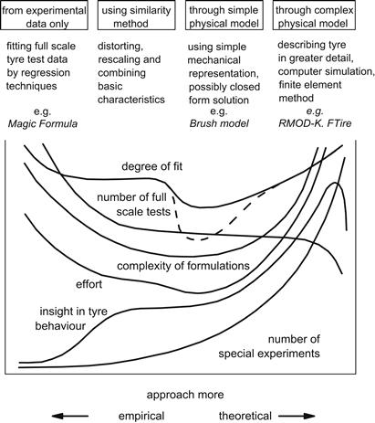
FIGURE 2.11 Four categories of possible types of approach to develop a tire model.
At the left-hand category, we have mathematical tire models that describe measured tire characteristics through tables or mathematical formulas and certain interpolation schemes. These formulas have a given structure and possess parameters that are usually assessed with the aid of regression procedures to yield a best fit to the measured data. A well-known empirical model is the Magic Formula tire model treated in Chapter 4. This model is based on a sin(arctan) formula that not only provides an excellent fit for the Fy, Fx, and Mz curves but in addition features coefficients that have clear relationships with typical shape and magnitude factors of the curves to be fitted.
The similarity approach (second category) is based on the use of a number of basic characteristics typically obtained from measurements. Through distortion, rescaling, and multiplications, new relationships are obtained to describe certain off-nominal conditions. Chapter 4 introduces this method, which is particularly useful for application in vehicle simulation models that require rapid (e.g., real-time) computations.
Depending on the type of the physical model chosen, a simple formulation may already provide sufficient accuracy for limited fields of application. The HSRI model depicted in Figure 2.12 developed by Dugoff, Fancher, and Segel (1970) and later corrected and improved by Bernard, Segel, and Wild (1977) is a good example. The figure illustrates the considerable simplification with respect to a more realistic representation of tire deformation (Figure 2.13) that is needed to keep the resulting mathematical formulation manageable for vehicle dynamics simulation purposes and still include important matters such as the representation of combined slip and a coefficient of friction that may drop with speed of sliding.
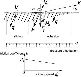
FIGURE 2.12 Top: The brush type tire model at combined longitudinal (brake) slip and lateral slip in case of equal longitudinal and lateral stiffnesses. Bottom: The linearly decaying friction coefficient.
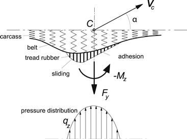
FIGURE 2.13 Tire model with flexible carcass at steady-state rolling with slip angle α.
The model of Figure 2.13 exhibits carcass flexibility and shows a more realistic parabolic pressure distribution. For such a model, (approximate) analytical solutions are feasible only when pure side slip (possibly including camber) occurs and the friction coefficient is considered constant (e.g., Fiala 1954).
Relatively simple physical models of this third category such as the ‘brush model’ of Figure 2.12 are especially useful to get a better understanding of tire behavior. The brush model with a parabolic pressure distribution will be discussed at length in Chapter 3.
The right-most group of Figure 2.11 is aimed primarily at more detailed analysis of the tire. The complex finite element- or segment-based models belong to this category (e.g., RMOD-K and FTire, cf. Chap. 13). A simpler representation of carcass compliance that is experienced in the lower part of the tire near the contact patch considerably speeds up the computation. In addition, the way in which the tread elements are handled is crucial. The computer simulation tread-element-following method is attractive and allows considerable freedom to choose pressure distribution and friction coefficient functions of sliding velocity and local contact pressure. The physical model that forms the basis of the latter method has been depicted in Figure 2.14.
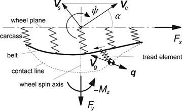
FIGURE 2.14 Computer simulation tire model with flexible carcass, arbitrary pressure distribution, and friction coefficient functions. Forces acting on a single tread element mass during one passage through the contact length are integrated to obtain the total forces and moment Fx, Fy, and Mz.
Influence (Green) functions may be used to describe the carcass horizontal compliance in the contact zone and possibly several rows of tread elements may be considered to move through the contact patch. One element per row is followed while it travels through the length of contact (or several elements through respective sub-zones). During such a passage the carcass deflection is kept constant, the motion of the single mass-spring (tread element) system that is dragged over the ground is computed, the frictional forces are integrated, the total forces and moment determined, and the carcass deflection is updated. Instead of using the dynamic way of solving for the deflection of the tread element while it runs through the contact patch, an iteration process may be employed. The model is capable of handling non-steady-state conditions. A relatively simple application of the tread-element-following method will be shown in the subsequent chapter when dealing with the ‘brush model’ subjected to combined slip with camber, a condition that is too difficult to deal with analytically. In addition, the introduction of carcass compliance will be demonstrated. A method based on modal synthesis to model tire deflection has been employed by Guan et al. (1999) and by Shang et al. (2002). For further study we refer to Sec. 3.3 and to the original work of Willumeit (1969), Pacejka, and Fancher (1972a), Sharp and El-Nashar (1986), Gipser et al. (cf. Sec.13.3), Guo and Liu (1997), and Mastinu (1997) and the state-of-the-art paper of Pacejka and Sharp (1991).
Although it is possible to develop a model for non-steady-state conditions by purely empirical means, most relatively simple and more complex transient and dynamic tire models are based on the physical nature of the tire. It is of interest to note that for a proper description of tire behavior at time-varying conditions an essential property must be represented in the physical models belonging to both right-hand categories of Figure 2.11. That is the lateral and sometimes also the fore and aft compliance of the carcass. Less complex non-steady-state tire models feature only carcass compliance without the inclusion of elastic tread elements. In steady-state models, the introduction of such a flexibility is often not required. Only to represent properly the self-aligning torque in case of a braked or driven wheel, is carcass lateral compliance needed. Tire inertia becomes important at higher speeds and frequencies of the wheel motion. The problem of establishing non-steady-state tire models is addressed in Chapters 5, 7, 8, 9, and 10 in successive levels of complexity to meet conditions of increasing difficulty.
Conditions become more demanding when for example: (1) the wheel motion gives rise to larger values of slip, which no longer permits an approximate linear description of the force- and moment-generating properties; (2) combined slip occurs, possibly including wheel camber and turn slip; (3) large camber occurs, which may necessitate the consideration of the dimensions of the tire cross section; (4) the friction coefficient cannot be approximated as a constant quantity but may vary with sliding velocity and speed of travel as occurs on wet or icy surfaces; (5) the wavelength of the path of contact points at non-steady-state conditions can no longer be considered large, which may require the introduction of the lateral and longitudinal compliance of the carcass; (6) the wavelength becomes relatively short, which may necessitate the consideration of a finite contact length (retardation effect) and possibly contact width (at turn slip and camber); (7) the speed of travel is large so that tire inertia becomes of importance, in particular its gyroscopic effect; (8) the frequency of the wheel motion has reached a level that requires the inclusion of the first or even higher modes of vibration of the belt; (9) the vertical profile of the road surface contains very short wavelengths with appreciable amplitudes as would occur in the case of rolling over a short obstacle or cleat, then, among other things, the tire enveloping properties should be accounted for; and (10) motions become severe (large slip and high speed), which may necessitate modeling the effect of the warming up of the tire involving possibly the introduction of the tire temperature as a model parameter. All items mentioned (except the last one) will be accounted for in the remainder of this book.