Basic Computer System Terms
Humpty Dumpty: “When I use a word, it means exactly what I chose it to mean; nothing more nor less.”
Alice: “The question is, whether you can make words mean so many different things.”
Humpty Dumpty: “The question is, which is to be master, that’s all.”
2.1 Introduction
Texts on computer systems introduce many more terms and concepts per page than do texts in other disciplines. This is a fundamental aspect of the field: Its goal is to recognize and define new computational structures and to refine those concepts. Besides the proliferation of terms, there is also widespread use of different terms to mean the same thing. Here are some synonyms one often encounters:
record = tuple = object = entity = …
block = page = frame = slot = …
file = data set = table = collection = relation = relationship =…
Of course, each author will maintain that a thread is not exactly the same as a task or a process—there are subtle differences. Yet the reader is often left to guess what these differences are.
In writing this book, we have tried to use terms consistently while mentioning synonyms along the way. In doing so, we have had to assume a basic set of terms. This chapter reviews those terms and defines them. All the terms presented here are repeated in the Glossary in a more abbreviated form.
This chapter also conveys our view that processors and communications are undergoing unprecedented changes in price and performance. These changes imply the transition to distributed client-server computer architectures. In our view, the transaction concept is essential to structuring such distributed computations.
The chapter assumes that the reader has encountered most of these ideas before, but may not be familiar with the terminology or taxonomy implicit in this book. Sophisticated readers may want to just browse this chapter, or come back to it as a reference for concepts used later.
2.1.1 Units
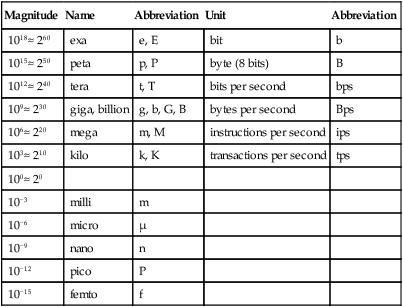
It happens that 210 ≈ 103; thus, computer scientists use the term kilo ambiguously for the two numbers. When being careful, however, they use k (lowercase) for the small kilo (103) and K for the big kilo (210). Similar ambiguities and conventions apply to mega and giga. Table 2.1 defines the standard units and their abbreviations and gives the standard names and symbols for orders of magnitude.
Table 2.1
The standard units and their abbreviations.
| Magnitude | Name | Abbreviation | Unit | Abbreviation |
| 1018≈ 260 | exa | e, E | bit | b |
| 1015≈ 250 | peta | p, P | byte (8 bits) | B |
| 1012≈ 240 | tera | t, T | bits per second | bps |
| 109≈ 230 | giga, billion | g, b, G, B | bytes per second | Bps |
| 106≈ 220 | mega | m, M | instructions per second | ips |
| 103≈ 210 | kilo | k, K | transactions per second | tps |
| 100≈ 20 | ||||
| 10−3 | milli | m | ||
| 10−6 | micro | μ | ||
| 10−9 | nano | n | ||
| 10−12 | pico | P | ||
| 10−15 | femto | f |
2.2 Basic Hardware
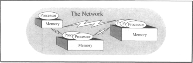
In Bell and Newell’s classic taxonomy [1971], hardware consists of three types of modules: processors, memory, and communications (switches or wires). Processors execute instructions from a program, read and write memory, and send data via communications lines. Figure 2.2 shows the overall structure of a computer system.
Computers are generally classified as supercomputers, mainframes, minicomputers, workstations, and personal computers. However, these distinctions are becoming fuzzy with current shifts in technology. Today’s workstation has the power of yesterday’s mainframe. Similarly, today’s WAN (wide area network) has the communications bandwidth of yesterday’s LAN (local area network). In addition, electronic memories are growing in size to include much of the data formerly stored on magnetic disk.
These technology trends have deep implications for transaction processing. They imply the following:
Distributed processing. Processing is moving closer to the producers and consumers of the data (workstations, intelligent sensors, robots, and so on).
Client-server. These computers interact with each other via request-reply protocols. One machine, called the client, makes requests of another, called the server. Of course, the server may in turn be a client to other machines.
Clusters. Powerful servers consist of clusters of many processors and memories, cooperating in parallel to perform common tasks.
Why are these computer architecture trends relevant to transaction processing? We believe that to be programmable and manageable, distributed computations require the ACID transaction properties. Thus, we believe that the transaction techniques described in this book are an enabling technology for distributed systems.
To argue by analogy, engineers have been building highly parallel computers since the 1960s. However, there has been little progress in parallel programming techniques. Consequently, programming parallel computers is still an art, and few parallel machines are in actual use. Engineers can build distributed systems, but few users know how to program them or have algorithms that use them. Without techniques to structure distributed and clustered computations, distributed systems will face the same fate that parallel computers do today.
Transaction processing provides some techniques for structuring distributed computations. Before getting into these techniques, let us first look at processor, memory, and communications hardware, and sketch their technology trends.
2.2.1 Memories
Memories store data at addresses and allow processors to read and write the data. Given a memory address and some data, a memory write copies the data to that memory address. Given a memory address, a memory read returns the data most recently written to that address.
At a low level of abstraction, the memory looks like an array of bytes to the processor; but at the processor instruction set level, there is already a memory-mapping mechanism that translates logical addresses (virtual memory addresses) to physical addresses. This mapping hardware is manipulated by the operating system software to give the processor a virtual address space at any instant. The processor executes instructions from virtual memory, and it reads and alters bytes from the virtual memory.
Memory performance is measured by its access time: Given an address, the memory presents the data at some later time. The delay is called the memory access time. Access time is a combination of latency (the time to deliver the first byte) and transfer time (the time to move the data). Transfer time, in turn, is determined by the transfer size and the transfer rate. This produces the following overall equation:
![]()
Memory price-performance is measured in one of two ways:
Cost/byte. The cost of storing a byte of data in that media.
Cost/access. The cost of reading a block of data from that media. This is computed by dividing the device cost by the number of accesses per second that the device can perform. The actual units are cost/access/second, but the time unit is implicit in the metric’s name.
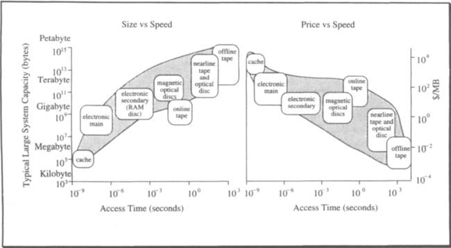
These two cost measures reflect the two different views of a memory’s purpose: (1) it stores data, and (2) it receives and retrieves data. These two functions are different. A device that does one cheaply probably is expensive for doing the other. Figure 2.3 shows the spectrum of devices and their price-performance as of 1990. Notice that the cost/byte and cost/access of these devices span more than ten orders of magnitude in capacities, access times, and cost/access.
Two generic forms of memory are in common use today: electronic and magnetic. Electronic memories represent information as charges or currents passing through integrated circuits. Magnetic memories represent information as polarized magnetic domains on a magnetic media.
Magnetic memories are non-volatile; they do not lose data if the power is turned off. Most electronic memory needs a power source to maintain the data. Increasingly, batteries are being added to electronic memories to make them non-volatile. The more detailed properties of these two memory technologies are discussed in the following two subsections. Discussion then turns to the way electronic and magnetic storage are combined into a memory hierarchy.
2.2.1.1 Electronic Memory
Byte-addressable electronic memory is generically called main memory, while block-addressable bulk electronic memory is variously called secondary storage, extended memory, or RAM disk. Usually, the processor cannot directly manipulate secondary memory. Rather, a secondary memory block (say, 10 KB) must be copied to main memory, where it is read and updated; the changed result is then copied back to secondary memory.
Electronic memories are getting much bigger. Gordon Moore observed that integrated circuit memory chips started out at 1 Kb/chip in 1970, and that since then their per-chip capacity has been increasing by a factor of four about every three years. This observation is now called Moore’s Law:
![]()
Moore’s Law implies that the 16 Mb memory chip will appear in 1991, and that the 1 Gb (gigabit) chip will appear in the year 2000. These trends have interesting implications for disks, for databases, and for transaction processing systems, but let us stick to processors and memories for a moment longer.
Memories are getting much bigger, while processors are getting faster. Meanwhile, inexpensive electronic memories are not getting much faster. Their access times are measured in tens of nanoseconds. Thus, a fast processor (say, a 1 bips machine) might spend most of its time waiting for instructions and data from memory. To mask this problem, each processor is given a relatively small, high-speed cache memory. This cache memory is private to the processor (increasingly, it is on the processor chip). The processor cache holds data and programs recently accessed by the processor. If most memory accesses “hit” the cache, then the processor will rarely wait for data from main memory.
The cache concept recurs again and again. Main memory is a cache for disk memories. Disk memories, in turn, may serve as a cache for tape archives.
2.2.1.2 Magnetic Memory
Magnetic memory devices represent information as polarized magnetic domains on a magnetic (or magneto-optical) storage media (see Figure 2.4). Some form of mechanical transport, called the drive, moves these domains past an electronic (or magneto-optical) read-write station that can sense and change the magnetic domains. This movement trades time for capacity. Doubling the area of the storage media doubles the capacity, but it also doubles the latency. Since magnetic media is very inexpensive, this time-space trade-off provides a huge spectrum of access time versus cost/byte choices (see Figure 2.3).

Two basic topologies are used to exploit magnetic media: the line (a tape) and the circle (a disk). The line has the virtue that it goes on forever (according to Euclid). The circle has the virtue that, as it rotates, the same point returns again and again. If the circle is rotated 100 times a second, the maximum latency for a piece of data to pass by the read station is 10 milliseconds. For a tape, the maximum read time depends on the tape length (≈1 km) and the tape transport speed. A maximum read time of one minute is typical for a tape. In general, tapes have excellent cost/byte but poor access times, while disks have higher cost/byte but better access times. In addition, magnetic tapes and floppy disks have become the standard media for interchanging data among computers.
Disks
Disk devices usually stack several (say, ten) platters together on a single spindle and then rotate them as a unit (see Figure 2.4). For each platter, the disk arm assembly has one read-write head, mounted on a fixed structure. The circle of data on a particular surface is called a disk track. As the disk platters rotate, the disk arm sees a cylinder’s worth of data from the many read-write heads. To facilitate reading and rewriting the data, each track is formatted as fixed-size sectors of data (typically about 1 KB). Sectors are the smallest read/write unit of a disk. Each sector stores self-correcting error codes. If the sector fails (that is, has an uncorrectable defect), a spare sector in the cylinder is used to replace it. The arm normally can move in and out across the platters, thereby creating hundreds or thousands of cylinders. This lateral movement is called seeking.
Disks have a three-dimensional address space: a sector address consists of (1) the cylinder number, (2) the track number within that cylinder, and (3) the sector number on that track. Disk controllers are getting more and more intelligent; they remap defects, cache recently read or written pages, and even multiplex an array of disks into a single logical disk to provide high transfer rates or high availability.
Modem disk controllers give a geometry-independent view of the disk. Such controllers have only two parameters: (1) the sector size and (2) the number of sectors. But the underlying three-dimensional geometry and performance of the disk has not changed. Consequently, disk access times are determined by three parameters:
![]()
High disk transfer rates come from disk striping, which partitions the parts of a large object among n disks. When the object is read or written, the pieces of it are moved in parallel to or from the n disks, yielding an effective transfer rate of n times the transfer rate of individual disks.
Today, average seek and rotation times are on the order of 10 milliseconds, rotation times are on the same order, and transfer rates are between 1 MBps and 10 MBps. These times are unlikely to change dramatically in the next decade. Consequently, access patterns to disks will remain a critical performance issue. To picture this, consider two access patterns to a megabyte of data stored in 1000 sectors of a disk:
Sequential access. Read or write sectors [x, x + 1, …, x + 999] in ascending order. This requires one seek (10 ms) and half a rotation (5 ms) before the data in the cylinder begins transfering the megabyte at 10 MBps (the transfer takes 100 ms, ignoring one-cylinder seeks). The total access time is 115 ms.
Random access. Read the thousand sectors [x, …, x + 999] in random order. In this case, each read requires a seek (10 ms), half a rotation (5 ms), and then the 1 KB transfer (.1 ms). Since there are 1000 of these events, the total access time is 15.1 seconds.
This 100:1 time ratio between sequential and random access to the same data demonstrates the basic principle: sequential access to magnetic media is tens or thousands of times faster than random access to the same data. Furthermore, transfer rates are increasing faster than access rates, so the speed differential between sequential and random access to magnetic media is increasing with time. This has two implications:
Big blocks. Transfer units for random accesses (block sizes) should be large so that transfer time compares to access time.
Data clustering. Great care should be taken by data management systems to recognize and preserve data clusters on magnetic media, so that the big blocks will move useful data (by prefetching it or postwriting it).
Chapter 13 explains how database systems use large electronic memories to cache most of the active data. While reads to cached data do not generate disk activity, writes generate a sequence of log records describing the updates. The log records of all updates form a single sequential stream of writes to magnetic storage. Periodically, the cached data is written to secondary storage (disk or nonvolatile electronic memory) as large sequential writes that preserve the original data clustering. This logging technique is now being applied to other areas, notably directory management of file servers.
A more radical approach keeps recently used data in electronic memory and writes changed blocks to magnetic storage in a sequential stream. This strategy, called a log-structured file system, converts all writes to sequential writes. Unfortunately, for many applications a log-structured file system seems to make subsequent reads of the archived data more random. There will be many innovations in this area as the gap between sequential and random access widens.
Our ability to read and write magnetic domains per unit area has been growing by a factor of ten every decade. This observation, originally made by Al Hoagland, is expressed in the formula:
![]()
Hoagland’s Law suggests that the capacity of individual disks and tapes will continue to increase. Of course, the exponential growth predicted by Moore’s Law, Hoagland’s Law, and Joy’s Law (Equations 2.3, 2.4, 2.8) must come to an end someday.
Tapes
Magnetic tape memories do not have the same high densities that magnetic disks have, because the media is flexible and not matched to the read-write head.1 Tapes, however, do have much greater area. In addition, this area can be rolled into a reel to yield spectacular volumetric memory densities (terabytes/meter3). In 1990, a typical tape fit in the palm of your hand and stored about a gigabyte.
Mounted tapes have latencies of just a few milliseconds to read or write data at the current position, in part because they use a processor to buffer the reads and writes. But the latency for a random read or write to a tape drive is measured in tens of seconds. Once a transfer starts, tape transfer rates are comparable to disk transfer rates (say, 10 MBps). Tapes, then, are the ultimate sequential devices. Tapes are typically formatted in blocks for error control and to allow rewriting.
Because a tape drive costs about as much as a disk drive (around $10/MB), tapes mounted on a tape drive have a relatively high cost/byte (see Figure 2.3). But when the tape is offline—removed from the reader—the cost/byte is reduced by a factor of a thousand, to just the cost of the media (around $10/GB). There is an intermediate possibility: nearline tape robots, which move a few thousand tapes between a storage rack and a few tape readers. The robot typically has between 2 and 10 tape drives and can dismount one tape and mount another in 40 seconds.
Tape robots are another example of trading time for space. The cost of the tape readers and the tape robot is amortized across many tapes (say, 10,000). If the robot costs $500,000, the unit cost of each tape is increased by a factor of six—from, say, $10 to $60 per gigabyte. The offline figure ignores the price of the reader needed for the offline tapes, as well as the cost of the four shifts of human operators needed to feed the reader. When those considerations are added, tape robots are very attractive.
2.2.1.3 Memory Hierarchies
The simple memory boxes shown in Figure 2.2 are implemented as a memory hierarchy (see Figure 2.5). Small, fast, expensive memories at the top act as caches for the larger, slower, cheaper memories used at lower levels of the hierarchy. Processor registers are at the top of the hierarchy, and offline tapes are at the bottom. In between are various memory devices, that are progressively slower, but that also store data less expensively.

A perfect memory would always know what data the processor needed next and would have moved exactly that data into cache just before the processor asked for it. Such a memory would be as fast as the cache. Memories cannot predict future references, but they can guess future accesses by using the principle of locality: data that was used recently is likely to soon be used again. By using the principle of locality, memories cache as much recently used data, along with its neighboring data, as possible. The success of this strategy is measured by the cache hit ratio:
![]()
When a reference misses the cache, it must be satisfied by accessing the next level in the memory hierarchy. That memory is just a cache for the next-lower level of memory; thus it, too, can get a miss, and so on.
Unless cache hit rates are very high (say, .99), the cache memory has approximately the same access time as the secondary memory. To understand this, suppose a cache memory with access time C has hit rate H, and suppose that on a miss the secondary memory access time is S. Further, suppose that C ≈ .01 • S, as is typical in Figure 2.3. The effective access time of the cache will be as follows:

Therefore, unless H is very close to unity, the effective access time is much closer to S than to C. For example, a 50% hit ratio attains an effective memory 50 times slower than cache; a 90% hit ratio attains an effective memory 11 times slower than cache. If the hit ratio is 99%, the effective memory is half as fast as cache. To achieve an effective memory speed within 10% of the cache speed, the hit rate must be 99.98%.
This simple computation shows that high hit ratios are critical to good performance. There are two approaches to improving hit ratios:
Clustering. Cluster related data together in one storage block, and cluster data reference patterns and instruction reference patterns to improve locality.
Larger cache. Keep more data in a larger cache, in the hopes that it will be reused.
Moore’s Law (Equation 2.2) says that electronic memory chips grow in capacity by a factor of four every three years. Hence, future transaction systems and database systems will have huge electronic memories. At the same time, the memory requirements of many applications continue to grow, suggesting that the relative portion of data that can be kept close to the processor will stay about the same. It is therefore unlikely that everything will fit in electronic memory.
The Five-Minute Rule
How shall we manage these huge memories? The answers so far have been clustering and sequential access. However, there is one more useful technique for managing caches, called the five-minute rule. Given that we know what the data access patterns are, when should data be kept in main memory and when should it be kept on disk? The simple way of answering this question is, Frequently accessed data should be in main memory, while it is cheaper to store infrequently accessed data on disk. Unfortunately, the statement is a little vague: What does frequently mean? The five-minute rule says frequently means five minutes, but the rule reflects a way of reasoning that also applies to any cache-secondary memory structure. In those cases, depending on relative storage and access costs, frequently may turn out to be milliseconds, or it may turn out to be days (see Equation 2.7).
The logic for the five-minute rule goes as follows: Assume there are no special response time (real-time) requirements; the decision to keep something in cache is, therefore, purely economic. To make the computation simple, suppose that data blocks are 10 KB. At 1990 prices, 10 KB of main memory cost about $1. Thus, we could keep the data in main memory forever if we were willing to spend a dollar. But with 10 KB of disk costing only $.10, we presumably could save $.90 if we kept the 10 KB on disk. In reality, the savings are not so great; if the disk data is accessed, it must be moved to main memory, and that costs something. How much, then, does a disk access cost? A disk, along with all its supporting hardware, costs about $3,000 (in 1990) and delivers about 30 accesses per second; access per second cost, therefore, is about $100. At this rate, if the data is accessed once a second, it costs $100.10 to store it on disk (disk storage and disk access costs). That is considerably more than the $1 to store it in main memory. The break-even point is about one access per 100 seconds, or about every two minutes. At that rate, the main memory cost is about the same as the disk storage cost plus the disk access costs. At a more frequent access rate, disk storage is more expensive. At a less frequent rate, disk storage is cheaper. Anticipating the cheaper main memory that will result from technology changes, this observation is called the five-minute rule rather than the two-minute rule.
The five-minute rule: Keep a data item in electronic memory if its access frequency is five minutes or higher; otherwise keep it in magnetic memory.
Similar arguments apply to objects stored on tape and cached on disk. Given the object size, the cost of cache, the cost of secondary memory, and the cost of accessing the object in secondary memory once per second, frequently is defined as a frequency of access in units of accesses per second (a/s):
![]()
Objects accessed with this frequency or higher should be kept in cache.
Future Memory Hierarchies
There are two contrasting views of how memory hierarchies will evolve. The one proclaims disks forever, while the other maintains that disks are dead. The disks-forever group predicts that there will never be enough electronic memory to hold all the active data; future transaction processing systems will be used in applications such as graphics, CAD, image processing, AI, and so forth, each of which requires much more memory and manipulates much larger objects than do classical database applications. Future databases will consist of images and complex objects that are thousands of times larger than the records and blocks currently moving in the hierarchy. Hence, the memory hierarchy traffic will grow with strict response time constraints and increasing transfer rate requirements. Random requests will require the fast read access times provided by disks, while the memory architecture will remain basically unchanged. Techniques such as parallel transfer (striping) will provide needed transfer rates.
The disks-are-dead view, on the other hand, predicts that future memory hierarchies will consist of an electronic memory cache for tape robots. This view is based on the observation that the price advantage of disks over electronic memory is eroding. If current trends continue, the cost/byte of disk and electronic memory will intersect. Moore’s Law (Equation 2.2) “intersects” Hoagland’s Law (Equation 2.4) sometime between the years 2000 and 2010. Electronic memory is getting 100 times denser each decade, while disks are achieving a relatively modest tenfold density improvement in the same time. When the cost of electronic memory approaches the cost of disk memory, there will be little reason for disks. To deal with this competition, disk designers will have to use more cheap media per expensive read-write head. With more media per head, disks will have slower access times—in short, they will behave like tapes.
The disks-are-dead group believes that electronic memories will be structured as a hierarchy, with block-addressed electronic memories replacing disks. These RAM disks will have battery or tape backup to make them non-volatile and will be large enough to hold all the active data. New information will only arrive via the network or through real-world interfaces such as terminals, sensors, and so forth. Magnetic memory devices will be needed only for logging and archiving. Both operations are sequential and often asynchronous. The primary requirement will be very high transfer rates. Magnetic or magneto-optical tapes would be the ideal devices; they have high capacity, high transfer rates, and low cost/byte. It is possible that these tapes will be removable optical disks, but in this environment they will be treated as fundamentally sequential devices.
The conventional model, disks forever, is used here if only because it subsumes the nodisk case. It asks for fast sequential transfers between main memory and disks and requires fast selective access to single objects on disk.
2.2.2 Processors
As stated earlier, processors execute instructions that read and write memory or send and receive bytes on communications lines. Processor speeds are measured in terms of instructions per second, or ips, and often in units of millions, or mips.
Between 1965 and 1990, processor mips ratings rose by a factor of 70, from about .6 mips to about 40 mips.2 In the decade of the 1980s, however, the performance of microprocessors (one-chip processors) approximately doubled every 18 months, so that today’s microprocessors typically have mips ratings comparable to mainframes (often in the 25 mips range). This rapid performance improvement is projected to continue for the next decade. If that happens, processor speeds will increase more in the next decade than they have in the last three decades. Bill Joy suggested the following “law” to predict the mips rate of Sun Microsystems processors to the year 2000.
![]()
In reality, things are going a little more slowly than this; still, the growth rate is impressive. Billion-instructions-per-second (1 bips) processors are likely to be common by the end of the decade.
These one-chip processors are not only fast, but they are also mass produced and inexpensive. Consequently, future computers will generally have many processors. There is debate about how these many processors will be connected to memory and how they will be interconnected. Before discussing that architectural issue, let us first introduce communications hardware and its performance.
2.2.3 Communications Hardware
Processors and memories (see Figure 2.2) are connected by wires collectively called the network. Regarded in one way, computers are almost entirely wires. But the notion of wire is changing: While some wires are just impurities on a chip, others are fiber-optic cables carrying light signals. The basic property of a wire is that a signal injected at one end eventually arrives at the other end. Some wires do routing—they are switches—while others broadcast to many receivers; here, the simple model of point-to-point communications is considered.
The time to transmit a message of M bits via a wire is determined by two parameters: (1) the wire’s bandwidth—that is, how many bits/second it can carry—and (2) the wire’s length (in meters), which determines how long the first bit will take to arrive. The distance divided by the speed of light in the media (Cm ≈ 200 million meters/s in a solid) determines the transmission latency. The time to transmit Message_Bits bits is approximately
![]()
Transmit times to send a kilobyte within a cluster are in the microsecond range; around a campus, they are in the millisecond range; and across the country, the transmit time for a 1 KB message is hundreds of milliseconds (see Table 2.6).
Table 2.6
The definition of the four kinds of networks by their diameters. These diameters imply certain latencies (based on the speed of light). In 1990, Ethernet (at 10 Mbps) was the dominant LAN.3 Metropolitan networks typically are based on 1 Mbps public lines. Such lines are too expensive for transcontinental links at present; most long-distance lines are therefore 50 Kbps or less. As the text notes, things are changing (see Table 2.7).
| Type of Network | Diameter | Latency | Bandwidth | Send 1 KB |
| Cluster | 100 m | .5 μs | 1 Gbps | 10 μs |
| LAN (local area network) | 1 km | 5. μs | 10 Mbps | 1 ms |
| MAN (metro area network) | 100 km | .5 ms | 1 Mbps | 10 ms |
| WAN (wide area network) | 10,000 km | 50. ms | 50 Kbps | 210 ms |

The numbers in Table 2.6 are “old”; they are based on typical technology in 1990. The proliferation of fiber-optic connections, both locally and in long-haul networks, is making 1 Gbps local links and 100 Mbps long-haul links economical. Bandwidth within a cluster can go to a terabit per second, if desired, but it is more likely that multiple links in the 1 Gbps range will be common. Similar estimates can be made for MANs and WANs. The main theme here is that bandwidth among processors should be plentiful and inexpensive in the future. Future system designs should use this bandwidth intelligently. Table 2.7 gives a prediction of typical point-to-point communication bandwidths for the network of the year 2000. These predictions are generally viewed as conservative.
Table 2.7
Point-to-point bandwidth likely to be common among computers by the year 2000.
| Type of Network | Diameter | Latency | Bandwidth | Send 1 KB |
| Cluster | 100 m | .5 μs | 1 Gbps | 5 μs |
| LAN (local area network) | 1 km | 5. μs | 1 Gbps | 10 μs |
| MAN (metro area network) | 100 km | .5 ms | 100 Mbps | .6 ms |
| WAN (wide area network) | 10,000 km | 50. ms | 100 Mbps | 50 ms |
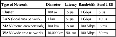
Table 2.7 indicates that cluster and LAN transmit times will be dominated by transfer times (bandwidth), but that MAN and WAN transmit times will be dominated by latency (the speed of light). Parallel links and higher technology can be used to improve bandwidth, but there is little hope of improving latency. As we will see in Section 2.6, cluster, LAN, and MAN times are actually dominated by software costs—the processing time to set up a message and the marginal cost of sending and receiving each message byte.
2.2.4 Hardware Architectures
To summarize the previous two sections, processor and communications performance are expected to improve by a factor of 100 or more in the decade of the 1990s. This is comparable to the improvement in the last three decades. In addition, the unit costs of processors and long-haul communications bandwidth is expected to drop dramatically.
2.2.4.1 Processor-Memory Architecture
How will these computers be interconnected? Where are processors in the memory hierarchy? How do processors fit into the communications network? The answers to these questions are still quite speculative, but we can make educated guesses. First, let us look at the question of how processors will attach to the memory hierarchy. Figure 2.8 shows three different strategies for this.
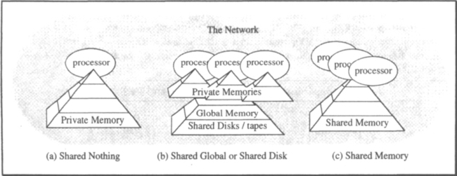
Shared nothing. In a shared-nothing design, each memory is dedicated to a single processor. All accesses to that data must pass through that processor.4 Processors communicate by sending messages to each other via the communications network.
Shared global. In a shared-global design, each processor has some private memory not accessible to other processors. There is, however, a pool of global memory shared by the collection of processors. This global memory is usually addressed in blocks (units of a few kilobytes or more) and is RAM disk or disk.
Shared memory. In a shared-memory design, each processor has transparent access to all memory. If multiple processors access the data concurrently, the underlying hardware regulates the access to the shared data and provides each processor a current view of the data.
Pure shared-memory systems will probably not be feasible in the future. Each processor needs a cache, which is inherently private memory. Considerable processor delays and extra circuitry are needed to make these private caches look like a single consistent memory. If, as often happens, some frequently accessed data appears in all the processor caches, then the shared-memory hardware must present a consistent version of it in each cache by broadcasting updates to that data. The relative cost of cache maintenance increases as the processors become faster.
One can picture this by thinking of the processor event horizon—the round-trip distance a processor can send a message in one instruction time. This time/distance determines how much interaction the processor can have with its neighboring processors. For a 1 bips processor, the event horizon is about 10 centimeters (≈4 inches). This is approximately the size of a processor chip or very small circuit board. Since wires are rarely straight, the event horizon of a 1 bips processor is on chip. This puts a real damper on shared memory.
As cache sizes grow, much of the program and data state of a process migrates to the cache where that process is running. When the process runs again, it has a real affinity to that processor and its cache. Because running somewhere else will cause many unneeded cache faults to global memory, processes are increasingly being bound to processors. This effectively partitions global memory, resulting in a software version of the shared-nothing design.
As a related issue, each device will be managed by a free-standing, powerful computer that can execute client requests. Requests will move progressively closer to the devices. Each keyboard and display, each disk, each tape robot, and each communications line will have its own dedicated processor. Consider, for example, the controller for a tape robot. This processor will manage an expensive device. The controller’s job is to optimize access to the device, deal with device failures, and integrate the device into the network. The controller will store a catalog of all the tapes and their contents and will buffer incoming data and prefetch outgoing data to optimize tape performance. Programming this software will require tools to reduce development and maintenance costs. Thus, the tape robot will probably run a standard operating system, include a standard database system, and support standard communications protocols. In other words, the tape robot controller is just a general-purpose computer and its software, along with a standard peripheral. Figure 2.9 diagrams this hardware.

Similar arguments apply to display controllers, disk controllers, and bulk electronic memory controllers (RAM-disks). Each is becoming a general-purpose processor with substantial private memory and a memory device or communications line behind it. Global memory devices are becoming processors with private memory.
2.2.4.2 Processor-Processor Architecture
Based on the previous discussion, shared-nothing and shared-global processors are likely to be grouped to form a single management entity called a cluster. The key properties of these clusters (see Table 2.7) are:
High communication bandwidth. Intra-cluster links can move bulk data quickly.
Low communication latency. Intra-cluster links have latency of less than 1 μs.
Clusters include software that allows a program (process) to access all the devices of the cluster as though they were locally attached. That is, subject to authorization restrictions, any program running in one processor can indirectly read or write any memory or wire in the cluster as if that device were local to the program. This is done by using a client-server mechanism. Clusters are available today from Digital (VAXcluster), IBM (Sysplex), Intel (Hypercube), Tandem (T16), and Teradata (DBC/1012).
Structuring a computation within a cluster poses an interesting trade-off question: Should the program move to the data, or should the data move to the program? The answer is yes. If the computation has a large state, it may be better to move the data than to move the process state; on the other hand, if the data is huge and the client process and the answer are small, then it is probably better to move the program to the data. Remote procedure calls are one way of moving programs so that they can execute remotely.
In summary, the processor-memory architecture is likely to move toward a cluster of shared-nothing machines communicating over a high-speed network. Clusters, in turn, communicate with other clusters and with clients via standard networks. As Table 2.7 suggests, these wires have impressive bandwidth, but they have large latencies because they span long distances. These trends imply that computations will be structured as clients making requests to servers. Remote procedure calls allow such distributed execution, while the transaction mechanism handles exceptions in the execution.
2.3 Basic Software—Address Spaces, Processes, Sessions
Having made a quick tour of hardware concepts, terms, and trends, let us look at the software analogs of the hardware components. Address spaces, processes, and messages are the software analogs of memories, processors, and wires. Following that basic client-server concepts are discussed.
2.3.1 Address Spaces
A process address space is an array of bytes. Each process executes instructions from its address space and can read and write bytes of the address space using processor instructions. The process address space is actually virtual memory; that is, the addresses go through at least one level of translation to compute the physical memory address.
Address spaces are usually composed of memory segments. Segments are units of memory sharing, protection, and allocation. As one example, program and library segments in one address space can be shared with many other address spaces. These programs are read-only in the sense that no process can modify them. As another example, two processes may want to cooperate on a task and, in doing so, may want to share some data. In that case, they may attach a common segment to each of their address spaces. Figure 2.10 shows these two forms of sharing. To simplify memory addressing, the virtual address space is divided into fixed-size segment slots, and each segment partially fills a slot. Typical slot sizes range from 224 to 232 bytes. This gives a two-dimensional address space, where addresses are (segment_number, byte). Again, segments are often partitioned into virtual memory pages, which are the unit of transfer between main and secondary memory. In these cases, virtual memory addresses are actually (segment, page, byte). If an object is bigger than a segment, it can be mapped into consecutive segments of the address space.

Paging and segmentation are not visible to the executing process. The address space looks like a sequence of bytes with invalid pages in the empty segment slots and at the end of partially filled segment slots.
Address spaces cannot usually span network nodes: that is, address spaces cannot span private memories (see Figure 2.8). Global read-only and execute-only segments can be shared among address spaces in a cluster. However, since keeping multiple consistent copies of a read-write shared segments is difficult, this is not usually supported.
2.3.2 Processes, Protection Domains, and Threads
Processes are the actors in computation; they are the software analog of hardware processors. They execute programs, send messages, read and write data, and paint pictures on your display.
2.3.2.1 Processes
A process is a virtual processor. It has an address space that contains the program the process is executing and the memory the process reads and writes. One can imagine a process executing C programs statement by statement, with each statement reading and writing bytes in the address space or sending messages to other processes.
Why have processes? Well, processes provide an ability to execute programs in parallel; they provide a protection entity; and they provide a way of structuring computations into independent execution streams. So they provide a form of fault containment in case a program fails.
Processes are building blocks for transactions, but the two concepts are orthogonal. A process can execute many different transactions over time, and parts of a single transaction may be executed by many processes.
Each process executes on behalf of some user, or authority, and with some priority. The authority determines what the process can do: which other processes, devices, and files the process can address and communicate with. The process priority determines how quickly the process’s demand for resources (processor, memory, and bandwidth) will be serviced if other processes make competing demands. Short tasks typically run with high priority, while large tasks are usually given lower priority and run in the background.
2.3.2.2 Protection Domains
As a process executes, it calls on services from other subsystems. For example, it asks the network software to read and write communications devices, it asks the database software to read and write the shared database, and it asks the user interface to read and write widgets (graphical objects). These subsystems want some protection from faults in the application program. They want to encapsulate their data so that only they can access it directly. Such an encapsulated environment is called a protection domain. Many of the resource managers discussed in this book (database manager, recovery manager, log manager, lock manager, buffer manager, and so on) should operate as protection domains. There are two ways to provide protection domains:
Process = protection domain. Each subsystem executes as a separate process with its own private address space. Applications execute subsystem requests by switching processes, that is, by sending a message to a process.
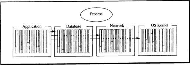
Address space = protection domain. A process has many address spaces: one for each protected subsystem and one for the application (see Figure 2.11). Applications execute subsystem requests by switching address spaces. The address space protection domain of a subsystem is just an address space that contains some of the caller’s segments; in addition, it contains program and data segments belonging to the called subsystem. A process connects to the domain by asking the subsystem or OS kernel to add the segment to the address space. Once connected, the domain is callable from other domains in the process by using a special instruction or kernel call.
The concept of an address space as a protection domain was pioneered by the Burroughs descriptor-based machines. Today, it is well represented by IBM’s AS400 machines, by the cross-memory services of the MVS/XA system, and by the four protection domains of the VAX-VMS process architecture. The concept of a process as a protection domain was pioneered by Per Brinch Hansen [1970] and is well represented by the UNIX operating systems of today.
Most systems use both process domains and address space domains. The process approach is the only solution if the subsystem’s data is remote or if the underlying operating system has a very simple protection model. But even that approach has at least two address spaces for each process: (1) the application domain and (2) the privileged operating system kernel domain that implements address spaces, processes, and interprocess communication. Typically, the hardware implements an instruction to switch from user mode to this privileged mode.
The process protection domain approach is the most general: it works in networks and in shared-memory systems. The drawback of using processes to implement protection domains is that a domain switch requires a process switch, and it may require copying parameters and results between the processes.
Structuring applications as multiple address space protection domains per process has real performance advantages. The multiple-address-space-per-process approach avoids most of these data copies. When the application calls the database system, the process assumes a new address space that shares the caller’s memory segments and the database system’s memory segments. The call begins executing at a standard location in the database system program. The database system can directly address the caller’s data as well as the database code and data. When implemented in hardware, such domain switches can be very rapid (≈100 instructions for a call plus return). This is much faster than the round-trip process switch, which involves several kernel calls and process dispatches. When the additional costs of parameter passing and authority checking are added, the cost of process switching rises substantially.
2.3.2.3 Threads
Address space protection domains show the need for multiple address spaces per process. There is a dual need for multiple processes per address space. Often the simplest way to structure a computation is to have two or more processes independently access a common data structure. For example, to scan through a data stream, one process is appointed the producer, which reads the data from an external source, while the second process processes the data. Further examples of cooperating processes, such as file read-ahead, asynchronous buffer flushing, and other housekeeping chores, are given in later chapters of this book.
Processes can share the same address space simply by having all their address spaces point to the same segments. Most operating systems do not make a clean distinction between address spaces and processes. Thus a new concept, called a thread or a task, is introduced to multiplex one operating system process among many virtual processes. To confuse things, several operating systems do not use the term process at all. For example, in the Mach operating system, thread means process, and task means address space; in MVS, task means process, and so on.
The term thread often implies a second property: inexpensive to create and dispatch. Threads are commonly provided by some software that found the operating system processes to be too expensive to create or dispatch. The thread software multiplexes one big operating system process among many threads, which can be created and dispatched hundreds of times faster than a process.
The term thread is used in this book to connote these light-weight processes. Unless this light-weight property is intended, process is used. Several threads usually share a common address space. Typically, all the threads have the same authorization identifier, since they are part of the same address space domain, but they may have different scheduling priorities.
2.3.3 Messages and Sessions
Sessions are the software analog of communication wires, and messages are the software analog of signals on wires. One process can communicate with another by sending it a message and having the second process receive the message.
Shared memory can be used to communicate among processes within a processor, but messages are used to communicate among processors in a network. Even within a processor, messages can be used among subsystems if the underlying operating system kernel does not support shared-memory segments (see Subsection 2.3.2.2).
Most systems allow a process to send messages to others. The send routine looks up the recipient’s process name to find its address—more on that below—and then constructs an envelope containing the sender’s name, the recipient’s name, and the message. The resulting envelope is given to the network to deliver, and the send routine returns to the caller. Such simple messages are called datagrams. The recipient process can ask the network if any datagrams have recently arrived for the recipient, and it can wait for a datagram to arrive.
More often, the communication between two processes is via a pre-established bidirectional message pipe called a session. The basic session operations are open_session(), send_msg(), receive_msg(), and close_session(). The naming and authentication issues of sessions are described in Section 2.4, but the basic functions deserve some comment here.
There is a curious asymmetry in starting a session. Once started, however, sessions are completely symmetric in that each side can send and receive messages via the session. The asymmetry in session setup is similar to the asymmetry in establishing a telephone conversation: one person dials a number, the other person hears the ring and picks up the phone. Once this asymmetric call setup is done and the two people have identified each other, the telephone conversation itself is completely symmetric. Similarly, in starting the session, one process, typically a server, listens for an open_session datagram from the network. Another process, call it the client, decides it wants to talk to the server; hence, the client sends an open_session datagram to the server and waits for a response. The server examines the client’s open_session request and either accepts or rejects it. Once the server has accepted the open request, and the client has been so informed, the client and server have a symmetric relationship. Either side can send at any time, and either side can unilaterally close the session at any time. The client-server distinction provides a convenient naming scheme, but the session endpoints are peers. The term peer-to-peer communication is often used to denote this equality.
Since datagrams seem adequate for all functions, why have sessions at all? The answer is that sessions provide several benefits over datagrams:
Shared state. A session represents shared state between the client and the server. The next datagram might go to any process with the designated name, but a session goes to a particular instance of that name. That particular process can remember the state of the client’s request. When the client is done conversing with the server, it closes the session, and the server waits for a new client’s open_session() request.
Authorization-encryption. As explained in the next section, clients and servers do not always trust each other completely. The server often checks the client’s credentials to see that the client is allowed (authorized) to perform the requested function. This authorization step requires that the server establish the client’s identity, that is, authenticate the client. The client may also want to authenticate the server. Once they have authenticated each other, they can use encryption to protect the contents and sequence of the messages they exchange from disclosure or alteration. The authentication and encryption protocols require multi-message exchanges. Once the session encryption key is established, it becomes shared state.
Error detection and correction. Messages flowing in each session direction are numbered sequentially. These sequence numbers can detect lost messages (a missing sequence number) and duplicate messages (a repeated sequence number). In addition, since the underlying network knows that the client and server are in session, it can inform the endpoints if the other endpoint fails or if the link between them fails. In this way, sessions provide simple failure semantics for messages. This topic is elaborated in the next chapter.
Performance and resource scheduling. Resolving the server names to an address, authenticating the client, and authorizing the client are fairly costly operations. Each of these steps often involves several messages. By establishing a session, this information is cached. If the client and server have only one message to exchange, there is no benefit. But if they exchange many messages, the cost of the session setup functions is paid once and amortized across many messages.
2.4 Generic System Issues
With the basic software concepts of process, address space, session, and message now introduced, the generic client-server topics of communication structure, naming, authentication, authorization, and scheduling can be discussed. Then particular topics of a file system and a communications system are covered in slightly more detail.
2.4.1 Clients and Servers
As mentioned earlier, computations and systems are structured as independently executing processes, either to provide protection and fault containment, or to reflect the geographic dispersion of the data and devices, or to structure independent and parallel computations.
How should a computation consisting of multiple interacting processes be structured? This simple question has no simple answer. Many approaches have been tried in the past, and more will be tried in the future.
One of the fundamental issues has been whether two interacting processes should behave as peers or as clients and servers. These two structures are contrasted as follows:
Peer-to-peer. The two processes are independent peers, each executing its computation and occasionally exchanging data with the other.
Client-server. The two processes interact via request-reply exchanges in which one process, the client, makes a request to a second process, the server, which performs this request and replies to the client.
The debate over this structuring issue has been heated and confused. The controversy centers around the point that peer-to-peer is general; it subsumes client-server as a special case. Client-server, on the other hand, is easy to program and to understand; it is fine for most applications.
To understand the simplicity of the client-server model, imagine that a program wants to read a record of a file. It can issue a read subroutine call (a procedure call) to the local file system to get the record’s value from the file. Virtually all our programming languages and programming styles encourage this operation-on-object approach to computing, in this case,
read(file, record_id) returns (record_value).
This programming model is at the core of object-oriented programming, which applies methods to objects. In client-server computing, the server implements the methods on the object. When the client invokes the method (procedure, subroutine), the invocation parameters are sent to the server as a message, then the server performs the operation and returns the response as a message to the client process. The invocation software copies the response message into the client’s address space and returns to the client as though the method had been executed by a local procedure.
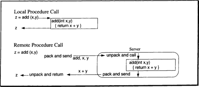
The transparent invocation of server procedures is called remote procedure call (RPC). To the client programmer (program), remote procedure calls look just like local procedure calls. The client program stops executing, and a message is sent to the server, which executes and replies to the client. On the server side, the invocation also looks just like a local procedure call. That is, the server thinks it was called by a local client. The mechanisms that achieve this are elaborated in Chapter 6, but the basic idea is diagrammed in Figure 2.12.
The RPC model seems wonderful. It fits our programing model, it is simple, and many standard versions of it are emerging. What, then, is the controversy about? Why do some prefer the peer-to-peer approach? The answer is complex. The client-server model postulates a one-to-one relationship between requests and replies. While this is fine for most computations, there are cases in which one request generates thousands of replies, or where thousands of requests generate one reply. Operations that have this property include transferring a file between the client and server or bulk reading and writing of databases. In other situations, a client request generates a request to a second server, which, in turn, replies to the client. Parallelism is a third area where simple RPC is inappropriate. Because the client-server model postulates synchronous remote procedure calls, the computation uses one processor at a time. However, there is growing interest in schemes that allow many processes to work on problems in parallel. The RPC model in its simplest form does not allow any parallelism. To achieve parallelism, the client does not block waiting for the server response; rather, the client issues several requests and then waits for the answers.
It appears that the debate between the remote procedure call and peer-to-peer models will be resolved by constructing the underlying mechanisms—the messages and sessions—on the peer-to-peer model, while basing most programming interfaces on the client-server model. Applications needing a non-standard model would use the underlying mechanisms directly to get the more general model.
One other generic issue concerning clients and servers deserves discussion here. Where do the servers come from? Here, there are two fundamentally different models, push and pull. In the push model, typical of transaction processing systems, the servers are created by a controlling process, the transaction processing monitor (TP monitor). As client requests arrive, the TP monitor allocates servers to clients, pushing work onto the servers. In the pull style, typical of local network file servers, an ad hoc mechanism creates the servers, which offer their services to the world via a public name server. Clients looking for a particular service call the name server. The name server returns the names of one or more servers that have advertised the desired service. The client then contacts the server directly. In this model, the servers manage themselves, and they pull work into the system. Pull results in higher server utilization since idle servers advertize for work, rather than having busy clients search for idle servers.
To summarize, the client-server structure lends itself to a request-reply programming style that dovetails with procedural programming languages. The server implements operations (methods, procedures) on objects, much in the style of object-oriented programming. The client invokes these procedures as though the objects were local, and the remote procedure call mechanism orchestrates the execution of the procedure by a remote server.
2.4.2 Naming
Every object, whether a process, a file, or a device, has a name, an address, and a location. The name is an abstract identifier for the object, the address is the path to the object, and the location is where the object is. As an example, the telephone named Bruce Lindsay’s Office has the address 408-927-1747 and is located at some electronic address inside IBM’s phone network. The name never changes, but Bruce may change locations, moving his telephone to a new office with the same phone number, or he may change addresses by going to MIT for a year.
An object can have several names. Some of these names may be synonyms, called aliases. Let us say that Bruce and Lindsay are two aliases for Bruce Lindsay. For this to be explicit, all names, addresses, and locations must be interpreted in some context, called a directory. For example, in our RPC context, Bruce means Bruce Nelson, and in our publishing context, Bruce means Bruce Spatz. Within the 408 telephone area, Bruce Lindsay’s address is 927-1747, and outside the United States it is +1-408-927-1747 (where the + stands for the international access code used to get to the root of the international telephone address space in the caller’s country).
Names are grouped into a hierarchy called the name space. An international commission has defined a universal name space standard, X.500, for computer systems. The commission administers the root of that name space. Each interior node of the hierarchy is a directory. A sequence of names delimited by a period (.) gives a path name from the directory to the object.
No one stores the entire name space—it is too big, and it is changing too rapidly. Certain processes, called name servers, store parts of the name space local to their neighborhood; in addition, they store a directory of more global name servers.
Clients use name servers to resolve server names to addresses. They then present these server addresses, along with requests, to the network. The network transports the requests to the server location, where it presents the request to the server (when the server asks for it). This is the scenario whereby sessions are established between clients and servers, and whereby remote procedure calls are implemented.
There is a startup problem: clients have to find the name and address of the local name server. To facilitate this, name servers generally have well-known names and addresses. A client wanting to resolve a name to an address sends a message to the well-known address or broadcasts the message to a well-known name on the local network. Once the name server responds to the client, the client knows the local name server’s address. The client can then ask the local name server for the addresses of more global name servers.
2.4.3 Authentication
When a client first connects to a server, each may want to establish the identity of the other. Consider the simple case of accessing your bank from your workstation. The bank wants to be sure that the person at the workstation is you, and you want to be sure that you are talking to your bank and not some Trojan horse that will steal your passwords and financial data. In computer terms, each process wants to authenticate the other: to establish the authorization identity, or authid, of the other. Every process executes under some authorization identity. This identity usually can be traced back to some person and, therefore, often is called the userid.
How can the client authenticate itself to a server? How can it convince the server of the client’s authorization identity? Conversely, how can the server convince the client? There are many answers to these questions, and there are many subtleties. Generically, however, there are two solutions: either (1) the client and the server must have a shared secret, or (2) the client and the server must trust some higher authority.
Passwords are the simplest case of shared secrets. The client has a secret password, a string of bytes known only to it and the server. The client sends this password to the server to prove the client’s identity. A second secret password is then needed to authenticate the server to the client. Thus, two passwords are required.
Another shared secret approach, called challenge-response,5 uses only one password or key. In this scheme, the client and the server share a secret encryption key. The server picks a random number, N, and encrypts it with the key as EN. The server sends the encrypted number, EN, to the client and challenges the client to decrypt it using the secret key, that is, to compute N from EN. If the client responds with N, the server believes the client knows the secret encryption key. The client can also authenticate the server by challenging it to decrypt a second random number. This protocol is especially secure because it sends only random numbers between the client and the server, no third party can see the shared secret. It may seem to introduce extra messages, but it turns out that the challenges and responses can piggyback on session-open messages, so that no extra message flows are needed.
A third scheme uses no shared secrets at all. Each authid has a pair of keys—a public encryption key, EK, and a private decryption key, DK. The keys are chosen so that DK(EK(X)) = X, but knowing only EK and EK(X) it is hard to compute X. Thus, a process’s ability to compute X from EK(X) is proof that the process knows the secret DK. Each authid publishes its public key to the world. Anyone wanting to authenticate the process as that authid goes through the challenge protocol: The challenger picks a random number X, encrypts it with the authid’s public key EK, and challenges the process to compute X from EK(X).
All these schemes rest on some form of key, but where do the keys come from? How do the client and the server get them securely? This issue, called key distribution, immediately brings some higher authority into the picture: someone or something that can make keys and securely distribute them. Such entities are called authentication servers. There are many different ways to structure authentication servers, but a fairly simple scheme goes as follows: The network is partitioned into authentication domains. Authorization identifiers become local to a domain in that an authorization identifier has a two-part name: (1) the authentication domain and (2) the authorization id within that domain. For example, if Sam is working in the government authentication domain called Gov, then Gov. Sam is Sam’s authid in the government authentication domain. All requests by Sam will be authorized against this authid. Authentication servers have a trusted way of securely communicating with each other so that they can certify these authids and their public keys. This communication mechanism is itself set up by some higher (human) authority.
A process acquires its authid by connecting to a local authentication server and authenticating itself. This authentication can be done via passwords, by challenge-response, or by some other scheme. Suppose a client in one authentication domain wants to talk to a server at a remote node and, at a remote authentication domain. Consider how the server authenticates the client: The server asks its authentication server for the client’s public key. The server’s authentication server asks the authentication server “owning” the client for the client’s public key. The authentication servers return the client’s public key to the server, which can then perform the challenge-response protocol. The main issue is trust—who trusts whom about what. In the scenario described above, trust takes two forms: (1) a process trusts its local authentication server to provide correct public keys, and (2) each authentication server trusts other authentication servers to provide the public keys of authids in their domains.
2.4.4 Authorization
What happens once a process has established an authid and a server has authenticated a client as having that authid? The server now knows who the client is and what the client wants to do. The question then becomes, Is the client’s authid allowed to perform that operation on that object? This decision, called authorization, can be expressed as the following simple predicate:
boolean = Authorize(object, authid, operation);
The Authorize() predicate can be viewed as a three-dimensional boolean array or as an SQL table. The array, called the access control matrix, is quite sparse and stores only the TRUE entries. Usually, a column of the array is stored with the object. That is, the authorization logic keeps a list of (authid, operation) pairs for an object, called the object’s access control list. Alternatively, SQL systems routinely keep a three-column privileges table indexed by (object, authid). Either scheme quickly answers the authorization question.
The object owner often wants to grant access to everybody, or to all bank tellers, or to everybody in his group. Thus far, we have not encountered the concept of an authority group—a list of authids, or a predicate on authids. The group concept eases administration of the access control matrix and collapses its size. For example, to grant everybody in group G read authority on object O, the (O, G, read) element would be added to the privileges table. When a member of the group wanted to read the object, the authorization test would check the requestor’s membership in group G.
Some systems, especially governmental ones, want to know each time an authentication or authorization step happens. At such points, a record or message about the step must be sent to a security auditing server, which collects this information for later analysis.
Once the authorization check has been passed, the requestor is given a capability to operate on the object. This capability is often just a control block stored in the client’s context at the server. For example, if the client opens a file, the server allocates a file control block, which indicates the read-write privileges of the client. Thereafter, the client refers to the control block by a token, and the server uses the contents of the control block to avoid retesting the client’s authority on each call. Occasionally, the client must be given the capability directly; an example is if the server does not maintain client state. In this case, the server generally encrypts the control block and sends it to the client as a capability. When the client later presents the encrypted control block, the server decrypts it, decides that it is still valid, and then acts on it.
When a client calls a server, the server may, in turn, have to call a second server to perform the client’s request. For example, when your client calls a mail server and asks it to send a file, the server has to get the file either indirectly from your client or directly from the file server. When the mail system server goes to the file server, the mail system wants to use your (the client’s) authority to access the file. A mechanism that allows a server to act with the authority of the client is called amplification. Amplification is difficult to control because of the question of how and when the server’s amplified authority gets revoked. However, some form of amplification is essential to structuring client-server computations.
2.4.5 Scheduling and Performance
Once a server starts executing a request, the performance of the server becomes an issue. From the client’s perspective, performance is measured by the server’s response time: the time between the submission of the request and the receipt of the response. Response time has two components: (1) wait time—the time spent waiting for the server or, once the server is executing, the time spent waiting for resources, and (2) service time—the time needed to process the request when no waiting is involved. As the utilization of a server or resource increases, the wait time rises dramatically. In many situations,6 the average response time can be predicted from the server utilization, p, by the formula,
![]()
Equation 2.10 is graphed in Figure 2.13. Notice that for low utilization—say, less than 50%—the response time is close to the service time, but then it quickly rises. At 75% utilization it is four times the service time, and at 90% utilization, it is ten times the service time.

There are two ways to improve response time: reduce service time or reduce wait time. This subsection deals primarily with ways to reduce wait time of critical jobs by scheduling them in preference to less-critical jobs. Each process has an integer priority, that determines how quickly the process’s resource requests will be granted. In general, a high-priority process should be scheduled in preference to a low-priority process, and processes with the same priority should be scheduled so that they all make approximately the same rate of progress. A typical scheme is for high-priority requests to preempt low-priority requests and for requests of the same priority to be scheduled using a round-robin mechanism. Batch jobs get low priority and run in the background, while interactive jobs get high priority and are serviced as quickly as possible.
Servers generally service clients in priority order. To do this, the server must have a queue of requests that it can sort in priority order. This, in turn, suggests that many clients are waiting for the server. Such waiting is exactly what priority scheduling tries to avoid. Rather than having a single server process, then, each request should have its own server process. This concept, called a server class, is discussed in Chapter 6. Server classes reduce queueing for servers.
What should the server priority be, once the server starts executing a client request? In many systems, the server has its own priority, independent of the client. Often, server priorities are high compared to any other priorities, so that services have short wait times. However, this approach—fixed server priorities—breaks down in a client-server environment. A low-priority client running on a workstation can bombard a high-priority server with long-running requests, creating a priority inversion problem: a server performing low-priority requests at high priority, thereby causing truly high-priority work to wait for the low-priority task to complete. The server should run requests at the client’s priority, or perhaps at the client’s priority plus 1, so that client requests are executed in priority order.
2.4.6 Summary
This section introduced several client-server issues. First, RPCs were defined and the general peer-to-peer versus RPC issue was reviewed. Then, the issues of naming, authentication, and authorization were sketched. Finally, the issue of scheduling clients and servers in a network was reviewed. The discussion now turns briefly to file systems in a client-server environment.
2.5 Files
Files represent external storage devices to the application program in a device-independent way. A file system abstracts physical memory devices as files, which are large arrays of bytes. Chapters 13–15 describe a transactional file system in detail. This section gives a brief background on standard file systems.
2.5.1 File Operations
Files are created and deleted by the create() and delete() operations. In reality, the create operation has a vast number of parameters, but for present purposes a file name will suffice. As discussed in the previous section, names are merely strings of characters that are resolved to an address by looking in some name server. The file system usually acts as a name server, implementing a hierarchical name space. A file server with the name “net.node.server” might implement a file named “a.b.c” with the resulting file name “net.node.server.a.b.c”. The local file system and remote file servers accept file creation operations in a manner similar to this:

Once created, a file can be accessed in one of two ways. The first approach is to map the file to a slot of a process address space, so that ordinary machine instructions can read and write the file’s bytes. Address spaces share memory by mapping the same file. For example, processes running a certain program map the binary version of that program to their address spaces. The operations for such memory-mapped files are something like this:

A second approach, and by far the most common, is to explicitly copy data between files and memory. This style first opens the file and then issues read and write file actions to copy the data between the file and memory. These are the approximate operations for such explicit file actions:
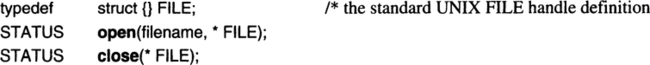
The execution of the open() routine gives a good example of the concepts of the previous section. When a client invokes the open() routine, code in the client’s library goes through the following logic: First, it must look up the name to find the file server owning that file. Often, the name is cached by the client library, but let us suppose it is not. In that case, the client asks the name server for the file server address. The client then sends the open request to the file server at that address. The file server authenticates the client and then looks for the file in its name space. If the file is found, the file server looks at the file descriptor, which, among other things, contains an access control list. The file server examines the file’s access control list to see if the client is authorized to open the file. If so, the file server creates a capability for the file (a control block that allows quick access to the file) and returns this capability to the client.
Given one of these file capabilities, the client can read and write bytes from the file using the following routines:

Notice that these are not exactly the UNIX routines; the standard UNIX read routine sequentially reads or writes the next bytes of the file. UNIX file positioning is done by a separate call, lseek(). Combined addressing and data copy operations are typical of random file access.
The two approaches, mapped files and explicit file access, are equivalent. The benefit of memory-mapped files is obvious: they make file access automatic. Historically, database implementors have preferred explicit access because database systems encapsulate files. Database systems carefully control file placement in memory (for clustering) and control data copies from memory to provide transactional file semantics. For 30 years, there has been a heated debate over whether memory-mapped files or explicit file access is better. The fact that this debate has continued for so long suggests that both approaches have merit.
2.5.2 File Organizations
A file system’s primary role is to store the contents of named files and to provide read and write access to them. File systems maintain other descriptive information about the file to control and direct access to it. As a rule, the file system keeps a descriptor for each file. The descriptor contains the file name, the authid of the file creator, and an access control list of who can do what to the file. The descriptor also keeps information on the time the file was created, when it was last accessed, and when it was last archived. Of course, the file size, along with a description of how the file is mapped to storage, is part of the descriptor.
File descriptors also cover the file contents. Often a file is unstructured; that is, it has no simple structure. For example, the binary image of a photograph has no regular structure; a simple byte stream file is likewise unstructured. By contrast, a structured file is a collection of records with similar structure. Structured files are dichotomized by their record addressing scheme: some file organizations address records associatively (by the record contents), while others only address records directly (by the record address in the file). Chapters 13–15 describe the semantics and implementation of structured files in considerable detail. The following simple description of structured files should suffice until then (see Figure 2.14).

Entry sequence is the simplest file structure. The name comes from the way records are inserted in the file. Each new record is added to the end of the file, so that the records are stored in the sequence they entered the file. Each record address is the byte offset of the record relative to the start of the file (or some similar scheme). Entry-sequenced files can be read sequentially—first record, second record, and so on—or a record can be directly addressed by using its byte offset.
Relative files are an array of records. Initially, the array is empty. When a record is inserted into a relative file, its array index must be specified as part of the insert. Subsequently, records can be read from the file either in array order or directly by array address.
Associatively accessed files are accessed via a record key composed of one or more subfields of the record. All records with a given key value can be quickly retrieved. Each time a record is inserted or updated, the record’s key is used to place the record in the file. There are two common record placement strategies, hashed and key-sequenced.
Hashed placement of records in a file is similar to hashing in main memory structures. The file is divided into an array of buckets. Given the key, one can quickly find the record by hashing the key to compute a bucket number and then searching that bucket for the record.
Key-sequenced placement stores the records sorted in key order. Key sequencing clusters related records together and allows sequential scanning of records in sorted order. Earlier sections of this chapter point out the benefits of this clustering and sequential access to data. When a new record arrives, its key is computed and the record is placed near records with related keys. Record insertion is a little expensive, but there are ingenious algorithms that make it competitive with hashing. Given a key value, it is easy to find the record by using binary search on the file or by using some indexing structure.
It is often desirable to associatively access a file via two different keys. For example, it is often convenient to access employees by either name or employee number. Suppose the employee records are stored in an associative file keyed by employee number (empno). Then a second associative file, keyed by employee name (empname), could store a record of the form <empname, empno> for each record in the employee file. By first looking in this second file under the empname key to find the empno, and then using this empno to associatively access the employee file, the system can fairly quickly find the desired employee record. Such index files are called secondary indices. It is often convenient to think of the direct address of a record as its key. If this is done, then secondary indices can be defined on direct files as well as on associative files.
Most systems allow file designers to define many secondary indices on a base file. The file system automatically maintains the records in the secondary indices as records are inserted into, updated in, and deleted from the primary file. Of course, the definition of the secondary index must be stored in the file descriptor. When a file is first opened, the descriptor is read by the server, and all subsequent record operations on the file cause the relevant secondary indices to be used and maintained.
2.5.3 Distributed Files
Parts of a file may be distributed among servers in a computer network. This distribution can take two forms: The files can be partitioned (fragments of the file are stored in different nodes), or the files can be replicated (the whole contents of the files are stored at several nodes).
The definitions of partitioning and replication are fairly simple. A file is broken into fragments by declaring the key boundaries of each fragment: All records within that key range belong to that fragment. For example, if a file is keyed by sales region and customer number, then the file might be fragmented by region, with each region having a separate fragment. These fragments might be partitioned among the computers of the various regions, with each region storing the fragment for that region. In addition, all the fragments might be replicated at central headquarters.
The descriptor of each fragment contains a complete description of the entire file. When a client opens the file, the file system looks at the descriptor and thereby knows about all the fragments. When the client issues a read-by-key, the request is dispatched to one of the servers managing that fragment. When the client issues a record insert, delete, or update operation, the request is dispatched to all servers managing the fragment that holds the record. Associated secondary index reads and writes are handled similarly.
If the file servers are transactional, then these update operations will be atomic, and the mutual consistency of the fragments, replicas, and their secondary indices will be maintained. If the file system is not transactional, then the fragments will quickly lose consistency as messages are lost or network nodes fail.
2.5.4 SQL
The record-oriented file system described previously is an advance over unstructured files, but it is still quite primitive. For example, the declaration of record attributes is often implicit, the logic to navigate via secondary indices is up to the client, and the client program is not insulated from changes to the file structure, such as adding or dropping indices.
There have been many attempts to raise the file-system level of abstraction. The current standard solution is the language SQL, which offers set-oriented, non-procedural data definition, manipulation, and control. (Subsection 1.3.5 gave a brief tour of SQL’s features.) The main point to be made here is that SQL is a software layer executed partly in a separate protection domain of the client process and partly in a server process (see Figure 2.15). SQL calls are much like file system calls in the sense that they create and delete SQL tables (similar to files) and read and write these tables. SQL tables are usually supported by the physical file organizations outlined in Figure 2.14. Portable SQL systems often begin with unstructured files and build everything from scratch. SQL systems, integrated with their operating system, typically add SQL semantics to the record structures of the native file system.
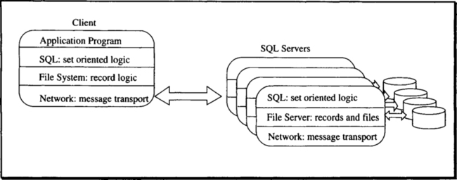
2.6 Software Performance
Having discussed all these concepts in the abstract, let us now give them some substance. How much does all this cost? How expensive is a message? How expensive is a process? How expensive is a transaction?
The performance issues in Section 2.2 were discussed in terms of hardware. Communications performance was measured by wire bandwidths and latencies. Memory performance was in terms of latencies and transfer rates of electronic and magnetic memories. Unfortunately, both for today and for many years to come, software dominates the cost of databases and communications. It is possible, but not likely, that the newer, faster processors will make software less of a bottleneck. This section gives a sense of typical software costs for storing and fetching records from a database, typical costs for sending a message, and typical costs for doing a remote procedure call. It also discusses how these numbers compare to latencies of the underlying physical devices.
In discussions such as this, it is important to distinguish carefully between what is possible and what is common. A research prototype with the fastest database or the fastest message system slows down as it becomes a product. This slowdown comes from adding maintenance features to the code (for example defensive programming), placing the code in its own protection domain, adding diagnostics, restructuring the code so that it is easy to understand and maintain, and so on. Figure 2.16 shows typical performance numbers from commercial systems.
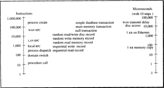
Figure 2.16 shows that RPCs are two or three orders of magnitude more expensive than local procedure calls. The figure also shows that with two 10-mips machines, sending a 1 KB message via Ethernet is limited by bandwidth rather than by processor speed. It shows that such machines can sequentially scan files at the rate of several thousand records per second, but that they only process a few hundred records per second in random order. Finally, it indicates that simple transactions (for example, the standard TPC-A transaction [Gray 1991]) require over 100,000 instructions to process, and that typical 10-mips systems can run about 50 such transactions per second.
When this discussion turns to future machines with 100 mips, or even with 1 bips, then all the instruction times decline by one or two orders of magnitude, bringing the software cost of a LAN RPC down to 100 or even 10 μs. As shown in Table 2.7, this is still more than the wire latencies for comparable communications in future clusters (≈5 μs), but is much less than MAN or WAN latencies (>500 μs) or disk latencies (>10,000 μs).
Perhaps the main conclusion to draw from this discussion is that the basic primitives discussed in this book—processes, sessions, messages, RPCs, transactions, files, records, SQL operations, and so on—are large operations. They are used for structuring a computation into a few fairly large steps.
The huge costs of these operations are not inevitable. There are lightweight analogs to most of these operations. Such lightweight systems sacrifice some of the niceties in favor of a ten-fold speedup. The resulting system is often called the fast-path. For example, IBM’s Transaction Processing Facility (TPF) can create a process in 1,000 instructions and can run the simple DebitCredit transaction in about 40,000 instructions. But this process is really a thread (no protection domains) running on a macro package to a very simple operating system. IBM’s IMS Fast Path system also runs that transaction in about 40,000 instructions by carefully optimizing the simple and common cases.
2.7 Transaction Processing Standards
Background in one more area is needed to understand distributed computing: standards for portability and for interoperation. There is a bewildering array of standards proliferating in our field. Two very important ones define a standard transactional client-server interface. They deserve to be introduced at this early stage.
2.7.1 Portability versus Interoperability Standards
This section gives a brief tour of the data communication standards relevant to transaction processing systems. Standards are defined with one or two goals in mind:
Portability. By writing programs in standard languages, the programs can be run on (ported to) many different computer systems.
Interoperability. By defining and implementing standard ways to exchange data, computers from different manufacturers can exchange data without any special conversion or interfacing code.
Programming languages such as FORTRAN, COBOL, and C are examples of portability standards. These standards require that when a program is ported to a new system, it must be recompiled for the instruction set and operating system of the new machine (as diagrammed in Figure 2.17).
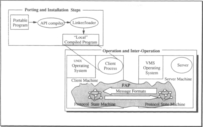
2.7.2 APIs and FAPs
Most communications standards are defined for interoperability. When two software or hardware modules want to communicate (interoperate), they must agree to both a common language, or set of messages, and a protocol to exchange these messages. Standards are defined to attain interoperation among many computer vendors and to minimize the number of different languages. In discussing standards, it is important to see the distinction between the programming interface, called the application programming interface or API, and the communication protocol, called the formats and protocols or FAP. The API is syntax, while the FAP is semantics. The API can be different at the two endpoints, but the FAP is a shared definition and must be the same at both endpoints. As an example from conventional programming, a Pascal program can call a C program. These programs have two different APIs (languages), but if they are to interoperate, they must agree on the way parameters are represented (for example, how arrays are mapped in storage), and they must agree on a procedure calling protocol and stack layout. In this simple case, then, the mechanics of procedure call are something like a FAP.
In communications, the FAP has two parts: (1) a detailed description of the message formats that flow on the wire or session between the endpoints, and (2) the protocol—a description of when these messages flow (see Figure 2.17). LU6.2 is further described in Subsection 16.3.5.
Message formats are the simple part of the FAP. For example, a FAP might say that a data message has the format

where integers are twos-complement binary integers, length is the number of bytes in the buffer field, and the buffer field is an array of characters encoded with ASCII byte encoding standard number 12345. The message formats give the exact encodings of information and the exact layout of these bits in a message.
Protocols are the major part of a FAP. They define in what order messages should be sent, how the two endpoints should act on receipt of each message, and how they should act on error conditions. To take a human example, a telephone call begins with the caller dialing the callee, waiting for a ring, waiting for an answer, conversing, and then hanging up. The callee waits for a ring, answers the phone, converses, and then hangs up. Rules for handling exception conditions (for example, wrong numbers, when the callee is busy, when the callee does not answer) must be specified. Rules to handle exceptions dominate protocol definitions.
Protocol rules are often described as a state machine plus an action for each state transition. The state machine is usually expressed as a decision table, where each state transition has a semantic action. The actions are defined in a procedural programming language. Typical events driving the state machine are arriving messages, time events, and client requests.
Application programmers never see the FAP; rather, they use an API to the FAP. The API is a set of subroutines that drive the state machine, or a special language that translates to such a set of subroutines. The API tends to vary from one language to another, because the host programming syntax and data types are different. For example, the COBOL interface is slightly different from the C interface (see Figure 2.17).
APIs come in many forms. Some, like C, COBOL, and SQL, are syntactic APIs; these are programming languages. Another form of API is a set of procedure calls or subroutines. UNIX, MS/DOS, and other operating systems are defined in this way. X-Windows and many other client-server systems are also defined by a standard call-level interface (CLI). The ultimate in portability is the definition of a CLI for a particular computer system: such an interface is called an application-binary interface (ABI). An ABI allows shrink-wrapped software to be installed on a machine without any special compilation steps and with a very simple linkage operation (linking the programs to the operating system library). MS/DOS on Intel 386 machines is the most common ABI today, but each computer family defines an ABI.
The respective benefits of a standard API and a standard FAP can be recapped in this way: A standard API makes a program portable, while a FAP allows two computers to interoperate. The concepts are orthogonal.
The proliferation of computers has created a comparable proliferation of communication standards. These standards can be classified as de jure standards—those defined by an international standards body—and de facto standards—those defined by an industry leader or an ad hoc consortium. It is common for a de facto standard to become a de jure standard over time. This happened to FORTRAN, SDLC, Ethernet, C, and SQL, and it is now happening in the transaction processing area.
2.7.3 LU6.2, a de facto Standard
Transaction processing communication standards provide an interesting example of these ideas. IBM has a de facto networking standard called Systems Network Architecture (SNA). SNA has many aspects, but one part of it defines a protocol to invoke remote transactional servers. This FAP, called LU (logical unit) 6.2, defines how a client can invoke a remote transactional server and establish a session with it. Since one server may invoke others, the set of servers and sessions forms a tree. LU6.2 specifies the formats and protocols to coordinate the atomic commitment of all members of such a tree of servers.
There are many application programming interfaces to LU6.2. They are generically called APPC (advanced program-to-program communication or application peer-to-peer communication). The original APPC implementation was done by IBM’s CICS and had a syntactic style API of the form

This syntactic standard requires a preprocessor (much as SQL does) and is not convenient for non-CICS environments. IBM adopted a procedural interface (a CLI) when it added LU6.2 to its standard list of programming interfaces. The result, known as common programming interface for communications (CPI-C), has a format like this:

The procedural standard varies only slightly from language to language, the variation being the different calling conventions and datatypes of each language. This CLI approach simplifies the API by eliminating a special compiler for the API (see Figure 2.17). CPI-C (pronounced sip-ich) standardizes the LU6.2 API across all computer environments.
2.7.4 OSI-TP with X/Open DTP, a de jure Standard
Subsequent to IBM’s SNA de facto standard, the International Standards Organization (ISO) has been defining a network architecture called Open Systems Interconnection (OSI). Several aspects of OSI define function in ways roughly equivalent to LU6.2 One standard, called Remote Operations Services (ROSE), defines how a client can invoke a server. Another standard, called Commit, Concurrency Control, and Recovery (OSI-CCR), defines the commit message protocols on a single session. A third standard, Transaction Processing (OSI-TP), defines how transaction identifiers should be created and managed. OSI-TP also specifies how commit should propagate in the tree of sessions and how session endpoints can resolve incomplete transactions after a failure. Fortunately, OSI-TP and LU6.2 are quite similar. To some extent, OSI-TP is a redefinition of LU6.2 in OSI terms. The redefinition repaired several minor LU6.2 flaws.
All the OSI standards of the previous paragraph are FAPs; they have no API. Thus, they allow transaction processing systems to interoperate, but they do not provide a way to write portable transaction processing applications or servers. A second standards body, X/Open, recognized this problem and is defining the X/Open Distributed Transaction Processing standard (X/Open DTP) to solve it. This standard defines the concept of resource managers coordinated by a transaction manager. Any subsystem that implements transactional data can be a resource manager (RM). Database systems, transactional file systems, transactional queue managers, and transactional session managers are typical resource managers. The transaction manager (TM) coordinates transaction initiation and completion among these resource managers. It also communicates with other transaction managers to coordinate the completion of distributed transactions.
X/Open DTP defines a library of procedures (a CLI) to begin a transaction, to declare a transaction abort, and to commit a transaction. This application-TM CLI is called the TX-interface. X/Open also defines a subroutine library for the resource managers to register with their local transaction manager, and for the transaction manager to invoke them at system restart and at transaction begin, commit, and abort. This TM-RM call-level interface comprises the so-called XA-interface. As described, this is sufficient for a portable, one-node transaction processing application or resource manager. Two mechanisms are needed for transactions or resources to be distributed: (1) a remote invocation mechanism and (2) a distributed transaction mechanism. Remote invocation is provided by ISO’s ROSE and by the many remote procedure call mechanisms. X/Open DTP specifies that the FAP for coordinating distributed transactions, the TM-TM interface, is OSI-TP.
The X/Open DTP design allows database vendors to write portable systems that act as resource managers and allow customers to write portable applications. It also allows vendors to write portable transaction managers. The standard is still evolving; this text attempts to follow its terminology and notation. A general picture of the X/Open DTP design is shown in Figure 2.18.
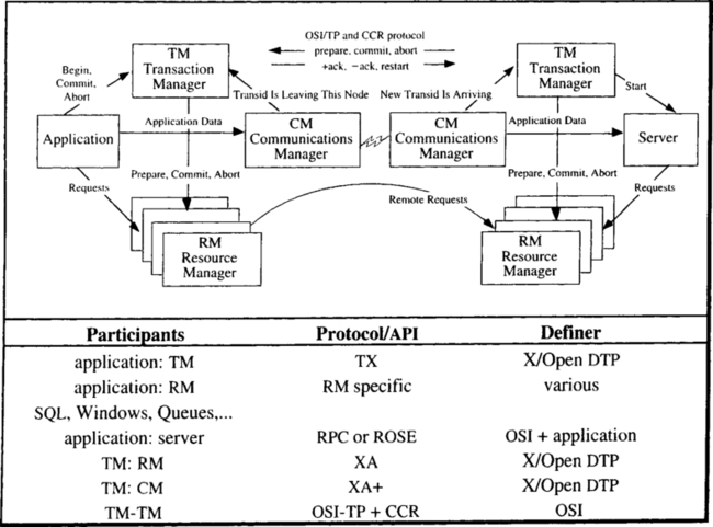
The work flow in X/Open DTP is approximately as follows. In the single-node case, an application invokes the TM to begin a transaction. It then invokes one or more resource managers, which may join the transaction. If the application fails, or if it asks the TM to abort the transaction, then the TM calls each resource manager and asks it to abort that transaction. If the application calls commit, then the transaction manager calls each resource manager and asks it to commit (see Figure 2.18).
If an application is distributed, then the application or a resource manager at one TM invokes an application or resource manager controlled by a second TM. In this case, both TMs are involved in the transaction commit. In order for the transaction managers to sense the distributed transaction, the communication managers (the network software) must inform them that the transaction is being distributed. This is shown in Figure 2.18, where the transaction manager on the left hears about the outgoing transaction identifier, and the transaction manager on the right hears about the incoming transaction identifier (this is called the XA+ interface). When the application commits or aborts, the two transaction managers will use the OSI-TP protocols to coordinate the transaction commit.
In summary, the combination of OSI and all its standards (notably ROSE, CCR, and TP) results in a transaction processing FAP. X/Open DTP provides a transaction processing API. To the reader unfamiliar with this material, the acronyms may be daunting. The important concepts to remember are that one mechanism, a FAP, is needed for interoperation, and a second mechanism, an API, is needed for portability.
A FAP can have many different APIs. Within the world of APIs, there are two kinds of interfaces: syntactic APIs like SQL, and procedural APIs like the UNIX libraries. Such procedural APIs are called CLIs, which stands for call-level interface. A CLI can be combined with an operating system definition and a machine definition to allow a standard binary interface for applications, better known as shrink-wrapped software. You can compile a program that uses the UNIX library and port it to any binary compatible UNIX machine. A syntactic API does not provide such binary compatibility. The source program must be recompiled on the target machine.
2.8 Summary
This chapter has covered the basic hardware and software concepts from the perspective of client-server distributed computing. Section 2.2 discussed hardware trends. It argued that the declining price of hardware is encouraging decentralization of computers by moving the processing and data closer to the data sources or consumers. These hardware trends also encourage structuring server machines as clusters of processors offering server interfaces to their data. The hardware discussion also introduced memory hierarchies and the technology trends of memory devices.
The basic software notions of address space, process, message, and session were then reviewed. With these concepts in place, the issues of client-server computing were outlined. First, remote procedure call was defined and contrasted with peer-to-peer structures. Then the issues of naming, authentication, authorization, and performance were surveyed, with particular focus on a client-server architecture.
This material was followed with a brief survey of file system terminology. File operations and organizations were described by way of introducing the standard types of files: keyed, hashed, relative, and entry sequenced.
The presentation then showed how expensive all these objects are. It pointed out that processes, RPCs, records, and transactions are large objects, consisting of many thousands of instructions. A computation is structured as, at most, a few hundred such operations per second. This is programing in the large.
The chapter ended with a brief tour of TP standards: This alphabet soup described the players and the current state of play. It mentioned the industry standard LU6.2 and CPI-C from IBM, as well as the de jure standards OSI-TP and X/Open DTP. It is important to be aware of these standards. They are treated in more detail in later chapters.
The underlying theme of Section 2.4 was that distributed computing is coming; in fact, it has already arrived. Distributed computing needs principles to structure it. Client-server, naming, authentication, authorization, and scheduling are essential techniques for structuring distributed computations. The transaction mechanisms described in the remainder of this book are also key to structuring distributed computations.
Exercises
1. [2.1, 5] A Kb is 2.4% bigger than a kb. How much bigger is a gb than a Gb?
2. [2.2.1.2, 15] Using Figure 2.3, compute the cost/access/second of a tape robot storing a nearline terabyte with a single tape drive. What if the robot has ten tape drives (and the same price)?
3. [2.2.1.2, 10] If a disk spins twice as fast, what is the new transfer rate, latency, and seek time? If mad increases by a factor of four what is the new transfer rate?
4. [2.2.1.2, 10] In the example of Subsection 2.2.1.2 comparing sequential to random access, sequential was faster by a factor of 151:1. Suppose the requests had been for a thousand 1 mb records rather than a thousand 1 kb records. What would the relative advantage of sequential be? At what transfer size is there a 10:1 advantage?
5. [2.2.1.3, 10] Given the cost/access for a tape robot, and given the costs for disks used in the discussion of the five-minute rule, and assuming that the object size is 1 mb, what is the break-even frequency for a tape robot at which it makes more sense to store the data on disk than to access it on tape each time? Assume the most optimistic cost/access for a tape robot from Problem 2.
6. [2.2.1.3, discussion] (a) Are disks dead? (b) Given Hoagland’s Law and Moore’s Law, and the prices from Figure 2.2, in what year will the laws intersect? (c) At that time, what will a tape look like in terms of capacity and latency?
7. [2.2.2, 10] The processor event horizon is the round-trip time/distance a signal can propagate between processor steps (clocks). This time/distance determines how much interaction the processor can have with its neighboring processors. What is the processor event horizon of a 1 bips processor given that the speed of light on a chip is about 2 • 108 m/s?
8. [2.2.3, 5] What fraction of the 1 kb send time is wire latency for a 1990 cluster or wan (Table 2.6)? What about the year 2000 cluster or wan?
9. [2.2.4, 25] Suppose a 1 bips processor has a big cache, which gives it 99% hit rates (a very good number). (a) What is the data request rate to main memory if each instruction generates two references? (b) If main memory has 20 ns access times, what is the effective cache speed? (c) Suppose a frequently accessed piece of data is stored in a shared ram disk as a 4 kb block, or it is stored in a server. The RAM-disk copy proceeds at 1 GBps, and so the processor can read or write it in 4 μs. Consider the read/write rules for the RAM-disk pages. What kind of synchronization is needed with other processors so that this processor can read and update the RAM-disk page? Suppose the ram disk is a processor itself, which accepts rpcs. What is the cost of doing a read or an update to the ram disk via rpc versus the cost of doing it via data reservation and moving?
10. [2.4.1, 10] Suppose a client wants to transfer a 1 mb file to a server over a wan with 50 ms one-way latency and .1 MBps transfer rate. Assume 1 kb message packets and ignore message addressing and checksumming overheads. Also ignore CPU time at the client and server. What is the best RPC time to transfer the file? What is the best peer-to-peer time to transfer the file?
11. [2.4.1, 10] Consider an rpc where the client uses four-byte one’s-complement integers and the server uses eight-byte two’s-complement integers. Who is responsible for the translation of the parameters? What if the translation is impossible?
12. [2.3.3, 5] Suppose my system uses passwords over Ethernet, as described in Subsection 2.4.3. (a) How would you break into my system? (b) It was mentioned that challenge-response messages can piggyback on open_session messages. How does that work?
13. [2.4.5, 10] In Subsection 2.4.5, there was considerable discussion of process priorities. Where do priorities come from? In a network, how does the server know the client priority? Does it make sense for separate threads in an address space to have separate priorities?
14. [2.4.5, 5] In Subsection 2.4.5 it was suggested that the server run at the client priority plus one? Why is that a good idea?
15. [2.5.2, 10] The end of Subsection 2.5.2 mentioned that implementors of structured files do not want to give users memory-mapped access to the files. Why?
16. [2.5.3, 10] Consider the accounts SQL table defined in Subsection 1.3.5.1. It was partitioned by primary key (account id). How would record read and insert be executed if the table were partitioned by customer number instead?
17. [2.6, 10] Suppose a transaction consists of an two LAN RPCs, four random in-memory record reads, and the null transaction overhead. Using Figure 2.16, what is the approximate instruction cost of such a transaction and what is its elapsed time on a 10 mips processor?
18. [2.6, 20] Suppose a transaction has a 5 ms service time and that there are no bottlenecks (resources that are 100% utilized and so limit the system throughput). Suppose the average transaction response time must be 100 ms or less. Using Equation 2.10, determine the maximum transaction throughput of the system that still satisfies this response time requirement. Do the same calculation for a processor that is ten times slower.
19. [2.7.1, 10] Shrink-wrapped software that you copy to a computer and then run immediately is the ultimate in portability. Suppose the program is stand-alone (no networking is involved). What standard interfaces do you need to write such a program? Hint: Such standards are called application binary interfaces (abis).
20. [2.7.1, 15] X/Open did not define an api for the tm-tm. It just specified a fap, namely osi-tp. Under what circumstances would the tm-tm interface need an api?
21. [2.7.2, 20] Try to design a fap for a human telephone. The fap should describe both the caller and the callee role. That is, unless the phone is “off hook,” the caller is a potential callee (if the phone rings). Proceed with this exercise as follows: (a) Write the error-free fap. (b) Pick five error cases, add them to your fap, and notice how much larger the program/decision table has grown. (c) Enumerate ten more error cases. (d) Based on the measurement sub-problem (b), extrapolate the size of the fap to handle these exceptions (note that the extrapolation is often combinatorial, not linear).
Answers
2. Robot access time is in the [30 second, 2 minute] range and access/second is between [.008,.033]. Cost per byte is in the [.01$/mb to 1$/mb] range. So the minimum cost is 10 k$ and the maximum cost is 1M$. The best case is 10,000/.033 ≈ 300 k$/a/s. The worst case is 120 m$/a/s. If the robot includes ten tape drives, these numbers drop by a factor of ten to between 30 k$/a/s and 12 m$/a/s.
3. Transfer rate is determined by how fast the bits pass the read-write heads. So double the spin doubles the transfer rate and cuts the latency in half, but it should not affect the seek time. If the magnetic area density increases by a factor of four, then the linear density doubles. So the transfer rate doubles, and the seek and latency are unchanged.
4. Computation is the same except that the total transfer time goes from 0.1 sec to 100 sec. The cost ratios are 100 seconds for sequential and 115 seconds for the random case, and the ratio is 1.15:1. At 10:1 the following equation holds: 10(L + 1000BT) = 1000(L + BT), where L is the latency and BT is the time to transfer a block. A little algebra gives BT = 1.65 ms. At 10 mb ps, this is a 16.5 kb block.
5. Using Equation 2.7, (Disk_Cost/Byte – Tape_Cost/Byte) • Object_Bytes = 10$ – .1$ = 9.9$. From Problem 2, the best cost/access is for the ten-drive robot and is about 30 k$/a/s, so frequently = (9.9/3 • 104) ≈ 1 access per 3,000 seconds, or about 1 access per fifty minutes. So a tape robot satisfies the fifty-minute rule.
6. (a) We don’t know. (b) About 2010. (c) 100 gb, same latency.
7. A 1 bips processor has a 10−9 clock, and the signal must travel out and back, so event horizon is 10−1 meters or 10 cm. This is approximately the size of a processor chip or a very small circuit board. Since wires are rarely straight, have capacitance and resistance, the event horizon of a 1 bips processor is about 1 cm. This puts a real damper on shared memory.
8. 1990: cluster: 5%; wan: 25%; 2000: cluster: 83%; wan: 100%.
9. (a) 20/ns, (b) 1.2 ns, (c) high!
10. A thousand rpcs are needed. They each have a 100 ms round-trip time, plus the message transmit time of 10 ms on a .1 MBps link. So each rpc needs 110 ms, and the total time is 110 seconds. In a peer-to-peer design, the client can send packets and the server can ack the last one. So the elapsed peer-to-peer time is about 10 seconds. This is the sort of example that makes peer-to-peer converts.
11. The rpc mechanism at the client or server must do the translation. If the translation is impossible (can’t fit 233 into a four-byte integer) then the rpc must signal an exception.
12. (a) To find passwords, tap the Ethernet, watch the passwords go by, and use them later. (b) In challenge-response, the client can send a challenge in the open message, the server can send a response and a challenge in the reply to the open message, and the client can send its response to the challenge on the first client request to the server.
13. Priority is a process-global variable. It is set by some administrative policy (e.g., person). The RPC invocation code should include the client priority in the message. The RPC receipt code should process requests in priority order and should set the server priority to the client priority plus one. Yes, different threads may be working for different clients and so should have different priorities.
14. It is desirable for servers to run at higher priority than clients so that clients do not preempt their servers or servers working for other clients with the same priority. If clients can preempt servers, server queues can get very long.
15. Access to structured files is complex, involving secondary indices, key lookups, and space allocation in a file. The file system wants to encapsulate these operations. The file system itself may run in a separate protection domain from the client, and the file system may memory map the files, but the file system does not want to give users byte-level access to the files. Incidentally, these issues are less relevant to clients with private files. They may not be willing to pay for the benefits of encapsulation.
16. The file would now be key sequenced on the account number key. Insert would send its update to the fragment based on the partitioning criterion. Sequential read of the table would be unchanged, but it would be in customer-number order. Read by customer number would send a read to the designated partition. To support read by primary key (account id) and to quickly test for primary key uniqueness, a secondary key-sequenced index would be created on the account id. This secondary index would be used to satisfy any read-by-primary-key requests. Maintenance of the secondary index would add extra work to any insert, update, and delete calls.
17. 2 LAN RPC ≈ 2 • 3,000 instructions; 4 random in-memory record accesses is ≈ 4 • 3000; null transaction is ≈30,000 instructions; so the total is 48,000 instructions or 4.8 ms.
18. The transaction response time must be about 100 ms, which is 20 times the basic service time. So, using Equation 2.10, 20 = 1/(1 – ρ), and so ρ = .95. Given that the machine is 95% utilized and that each transaction uses 5 ms (.5%), the system should be able to run (.95/.005) = 190 transactions per second. If the processor is 10x slower, the service time becomes 50 ms, the expansion factor is 2, ρ = .5, and the system can run (.5/.05) = 10 transactions per second. Notice that a 10x increase in power gives a 20x rise in throughput. This phenomenon is called transaction acceleration. If the processor is 10x faster, the expansion is 200, ρ = .995, and the throughput is 1,990 transactions per second. Notice that at the high end, the tps scales almost linearly with service time. It is only for ρ <.9 that the transaction acceleration is dramatic.
19. The program must be a binary, so the instruction set of the machine must be standardized. The format of runable binary programs must be standardized. The operating system interface to launch the program and any external libraries used by the program must be standardized. ms/dos defines such a standard for the Intel x86 series of processors, MacOS and SunOS have comparable standards.
20. The goal of X/Open dtp was portable applications and portable resource managers. X/Open views transaction managers as integrated with the host system and not portable, so only an interoperability standard was defined. The tm interfaces to the other tm via a communications manager implementing the osi protocols (rose, ccr, tp, and so on). These interfaces are extensive and complex. X/Open decided to avoid defining an API to each of them. Others are defining an RPC interface among tms to allow portable tms.
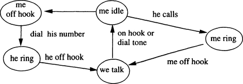
(b) Five interesting errors are: On the caller side, no dial tone, wrong number, nonexistent number, no answer after five rings, right number but wrong person. On the callee side, he hangs up just as I answer, we speak different languages (so I cannot understand him), we have a bad connection (so I cannot understand him), … (d) These errors tend to make the state machine much bigger. Often a single error can add transitions to many states.
1Tapes are undergoing a revolution in 1991 by increasing from 100 MB linear objects to 10 GB objects. This change is the result of switching to VCR helical scan technology and other recording innovations. This section was written in anticipation of that transition.
2This is the approximate scalar performance of IBM 360 processors (or their descendants in the IBM System/9000) when running scalar (as opposed to scientific) programs, such as SQL requests or a COBOL compilation.
3Note here that the discussion has switched from bytes (B) to bits (Mb).
4An exception: In some shared nothing systems, if a processor fails, some of its memory may be accessible to another processor.
5Challenge-response is the basis of IBM’s SNA authentication mechanism.
6The assumptions are m/m/1: Poisson arrivals, negative exponential service times, and a single server [Highleyman 1988].