
15.5 Sample Implementation of Some Operations on B-Trees
This section illustrates the implementation of a B-tree by presenting the details of two of its key functions, readkey and insert, including the split operation. The algorithms are expressed in pseudo-code and in C, depending on what is assumed to be obvious and what requires (from our perspective) some more elaboration. But note that even the C-code programs must not be mistaken as a real-life implementation of a B-tree; the entry structure has been simplified considerably to avoid the complications resulting from variable-length entries, since this is not specific for the functional principles of B-trees. For the same reason, most of the error checking and logic for special cases has been omitted. The main purpose of the programs is to illustrate unambiguously how the data structure of a B-tree is used and maintained, and how various components of the system—the B-tree manager, the record manager, the log manager, the buffer manager, and the lock manager—interact in its implementation.
15.5.1 Declarations of Data Structures Assumed in All Programs
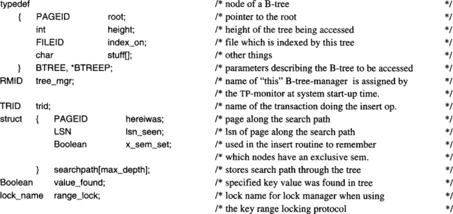
Let us start by declaring the variables and data structures needed. These declarations, in turn, refer to other declarations, such as page headers, log records, buffer control blocks, and so on, which have been discussed earlier. Here is the list of basic variables and control blocks needed.

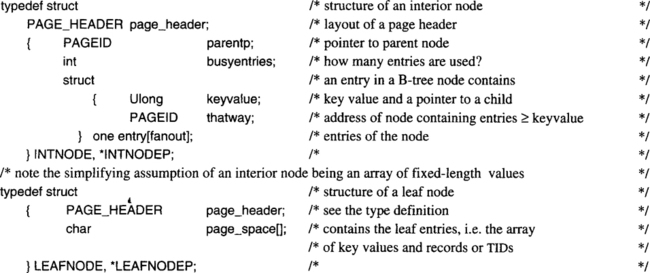
The parameters used to invoke the B-tree routines, and the result variables returned, are described by the following declarations:
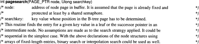
Access to the nodes in a B-tree is assumed to be implemented in two subroutines; these are not spelled out in C because they do not contain any aspects that are interesting from a transaction processing perspective. The first one, pagesearch(), gets as parameters a pointer to a page in buffer and a requested key value. It returns the index of an entry in the page according to the following convention: if the page is an index node, the index denotes the entry that contains the proper pointer to the next-lower layer in the traversal sequence. If it is a leaf page, the index denotes the entry that either contains the specified value (if it is present), or the entry that would have to receive that value in case of an insert. The prototype declare is given here:
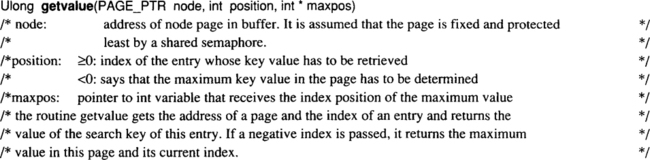
The second routine, getvalue, serves two purposes: first, it simply returns the key value from a leaf page, given its index. Second, it finds the maximum key value currently stored in a node and returns both that value and its index in the page.
In what follows, these routines are used without further explanation. Exception handling is omitted. Since the results they produce are fairly obvious, the discussion of B-tree implementation should be understandable without any additional functional details.
15.5.2 Implementation of the readkey Operation on a B-Tree
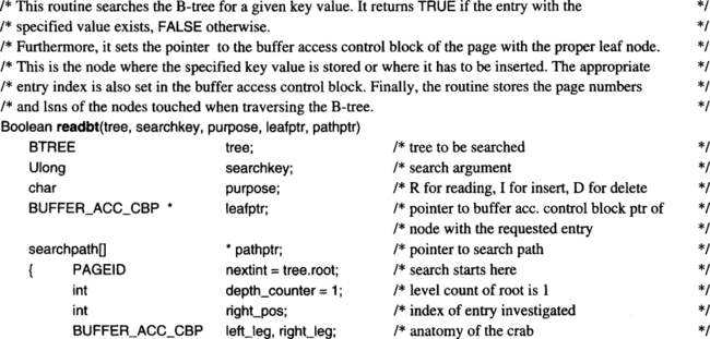
The readkey() function has to go through some logic having to do with the file descriptor, cursor management, and so on; these details are omitted here. For simplicity, it is assumed that the root page number of the tree and its height have already been determined from the file descriptor. With this, an internal routine, readbt(), is invoked. This routine will also be used by the insert function to determine the insert position. It returns the pointer to the buffer access control block of the page with the entry—that page is fixed and protected by a semaphore. It also returns the index of the entry with the key value or the index of the entry after which the search key value would have to be inserted; this parameter is passed via the index entry of the buffer access control block in the parameter list.
The return code of readbt() is FALSE if no match was found, TRUE if a match was found. For simplicity, it is assumed that the tree implements a unique index; there is no checking if more than one entry matches the search argument. We also ignore the special case of a single-page tree, where leaf and root coincide.
Since a full B-tree implementation with all provisions for synchronization, recovery, and so forth, is a fairly complex piece of code, the following explanation is based on pseudo-code rather than C-code, used in the previous chapters. The pseudo-code is close to C, though, whenever the use of an interesting data structure or interface is discussed. Otherwise, the statements are high-level references to explanations that are given in Section 15.4. Code that is at the C level is printed in the same font as the other C code in this book; for the pseudo-code, the text font is used.
The pseudo-code implementing the traversal of a B-tree in order to determine the page and index position of an existing key value, or the insert position of a new key value, follows the next paragraph. Except for getvalue(), the routine invokes a number of lower-level services: bufferfix(), bufferunfix(), and pagesearch().
Since the pagesearch() routine has not been spelled out completely, we must explain the meaning of the index in the leaf page that is returned in its buffer access control block. If the requested key value is found, it is the index of the entry containing that value. If searchkey is not found, the index points to the entry with the next-higher key value. We must also consider the situation in which searchkey is larger than any key value in the tree; in that case, there is no next page to crab to. This is taken care of by some reserved value representing “infinity,” that is, a value larger than any legal value of the index attribute domain. This value can also be used for next-key locking. Again, this technique is assumed without further explanation. The problems that can arise when crabbing along the leaf level are discussed in Subsection 15.4.4.3.

15.5.3 Key-Range Locking in a B-Tree
The readbt() routine is not all that is required to implement the readkey() access, although it does most of the work. The rest has to do with error handling, which is omitted here, and locking, which needs some explanation. According to the protocol explained in this chapter (see Table 15.12), the retrieved key value has to be locked in S mode in case the value was found. Otherwise, the enclosing key range must be locked by locking the next-lower value to avoid phantoms. To do this, we assume another ancillary routine that makes lock names from key values in accord with the declares in Chapters 7 and 8. The function prototype looks like this:

The preceding calls demonstrate the mainline logic used to access a B-tree and to synchronize these accesses using the next-key locking protocol introduced in Subsection 15.4.4. Of course, subsequent lock requests on the tuple pointed to by the B-tree must also be issued, but since these issues have nothing to do with B-tree management, they are ignored here.
The use of the timeout parameter in the invocation of the lock manager needs some explanation. As discussed earlier, one should not wait for a (potentially long) lock while holding a page semaphore. With the interfaces to the lock manager introduced in Chapter 8, there is no clean way to avoid this. We need bounce mode locks to achieve the desired effect: a lock request is issued, and it returns immediately with an indication if the object is already locked by another transaction. Issuing the lock request with a timeout interval of zero gives bounce mode locking, and that is why this trick is used here. If the transaction accessing the B-tree actually has to wait for the lock, it first gives up the semaphore, then requests the lock again (this time with a reasonable timeout), and, of course, has to verify that the leaf page has not changed while the transaction was waiting for the lock. This verification is done by comparing the leaf page’s LSN with the LSN of the same page after it has reacquired the semaphore. If the LSN has changed, the page must be reanalyzed. It can be the case that the desired entry is still in the page—the intermediate update has affected another entry. If this is so, processing proceeds normally. Otherwise, the client has to give up and retry the retrieval operation by going through readbt again.
Note that in case the lock is successfully acquired, the translation still holds a semaphore on the leaf page. The actual code hiding behind the phrase “prepare the results” must make sure that the lock gets released properly and the page is unfixed. If the key value was not found, the implementation may also decide to release the read lock on the next key, depending on what kind of read operation the transaction is executing. It was shown in Section 15.4 that there are situations where it is safe to proceed in that fashion.
15.5.4 Implementation of the Insert Operation for a B-Tree: The Simple Case
The routine that inserts a new tuple (or a reference to the tuple) into a B-tree structure first calls readbt to get the leaf page required and the index position in the page where the new tuple has to go (see Subsection 15.5.3). The readbt() routine ensures that there is an exclusive semaphore on the leaf node page and returns the path from the root to the leaf in the structure searchpath, which is passed via the variable pathptr in the parameter list. The function prototype declaration of this routine looks like the following:
For the reasons mentioned previously, all aspects related to handling the actual tuple are ignored here, because they are largely independent of the properties of the B-tree access path structure.
We present the implementation of the inserto routine as a sequence of code blocks. The explanation of the implementation issues starts with the simplest case, which is the insertion of the new entry somewhere in a leaf page; that is, special cases such as the new entry being the highest value in a leaf are ignored. Given this standard path through the insert logic, we will then consider some more complicated situations, such as page splits. Again, all the following considerations are based on the assumption that the B-tree implements a unique index and that the tuples are stored somewhere else; that is, the tree only contains TID references to the tuples. The logic for the simple case looks like this:


Let us now consider the case of an insert that requires a leaf to be split. To keep the discussion simple, the code is restricted to a leaf split only. This is justified by the fact that splitting an intermediate node requires the same essential steps as splitting a leaf node—with the exception of the root.
15.5.5 Implementing B-Tree Insert: The Split Case
The first thing that needs to be done is to protect all the nodes that will be affected by the split with exclusive semaphores. When it is discovered that a page must be split, only the leaf to be split has such a semaphore. This must be released, because the search path is revisited top-down based on the entries in searchpath, and we want to avoid deadlocks among transactions requesting semaphores. Once the nodes to be updated are covered by semaphores, the actual split can be performed and, finally, the semaphores can be released. The pseudo-code portion for the leaf node split implementing the techniques described in Subsection 15.4.1 is presented on the next page (the previous declares are assumed without repeating them).
This piece of code needs some additional comments. First, the idea of releasing the exclusive semaphores on those interior nodes that are not affected by the split rests on a critical asumption: one must be able to tell whether or not the discriminating key being propagated from the lower layer fits into the node before one actually knows which discriminating key that is. If all keys have fixed length (which, for simplicity, was assumed here), this is trivial.
If their keys have variable length (and if key compression is used), then it is not possible, in general. If it is not possible to safely decide whether or not an interior node has to be split, then either the entire search path (including the root) must be protected by an exclusive semaphore, or semaphores must be acquired bottom-up during the split processing, which requires means to detect deadlocks involving both locks and semaphores.
Second, it must be noted that there is a subtle problem with the ancillary routine getfreepage that returns the PAGEID of an empty page in the file holding the B-tree. Free page administration is typically done by the tuple-oriented file system, which probably is a different resource manager than the B-tree manager. Consequently, it does its own logging. If it does log the allocation operation in the conventional manner, then there is a problem if the transaction in which the split occurs is later rolled back. The B-tree manager logically undoes the insert but does not revert the split; the file manager, however, would do its part of the rollback, which implies claiming the empty page again. On the other hand, if the file manager does no logging and the transaction crashes early, empty storage might be lost. Therefore, a cooperation between the two components is needed; this cooperation can be defined in different ways. One possibilty is to give the authority for free page management to the B-tree manager; this means that from the file system’s perspective, the B-tree manager claims all the space right away and keeps track of which pages are used and which are not. Then, there is no problem in recovering allocation operations according to the scheme introduced here. Another possibility is to enclose the allocation operation (done by the file system) and the log write for the allocation (done by the B-tree manager) into one common, nested top-level transaction. Then, two things can happen: either the page is allocated and the B-tree manager’s log record for it is written, which means it can explicitly return that page if the closing parenthesis is missing after a crash; or the nested top-level transaction fails, in which case normal UNDO will take care of recovery.


The point about the code here has to do with splitting higher-level nodes. In our example, the operation “modify parent” is assumed to affect only one node. In general, however, it would have to call the split routine recursively, until the level recorded in split_up_to is reached. For each split operation on the way, the same logic is applied. A new opening parenthesis is written to the log, identifying the page to be split; all the log records pertaining to that split are recorded the same way; and so on. In effect, the log will contain nested parentheses, and the insert is complete only if the outer closing parenthesis is found.
15.5.6 Summary
The implementation section has presented (pseudo-) code pieces to illustrate the application of the guiding principles for implementing transactional resource managers: the use of semaphores and logging to perform consistent, isolated, and atomic page changes; the combination of low-level locks (semaphores) and key-range locks to achieve high concurrency on a popular data structure such as a B-tree; the combination of physical REDO and logical UNDO to reduce lock holding times.
15.6 Exotics
Considering which access paths are actually used in real transaction processing systems, the vast majority of algorithms proposed in the literature must be classified as exotic. This may be a bit unfair though, because the decision about which access mechanisms to include in a system is influenced by many criteria, many of which are nontechnical. Given the fact that B-trees provide the optimal balance between functionality and cost, the question usually is, What else?
The obvious answer is that something with the best performance is needed; this favors a decision for static hashing. Beyond hashing and B-trees, it is not trivial to identify requirements that justify the implementation costs of yet another associative access path technique. It would have to be a performance requirement or a functional property that neither hashing nor B-trees can fulfill properly, because no new access path will be implemented in a real system if it is just slightly better under some special circumstances. To appreciate that, the reader should rethink the whole discussion on B-trees. It demonstrates that using an access method in a general-purpose transaction system means much more than just coding the search algorithms. The additional transaction-related issues, such as synchronization and recovery, can turn out to be more complicated than maintaining the search structure itself. And furthermore, for each new access method, there must be an extension of the SQL compiler and optimizer to decide when to use this type of access path and to generate code for it.
New access methods, then, will only be justified (and implemented) if there are applications with performance requirements that neither static hashing nor B-trees can meet, or if there is a requirement for types of associative access that exceed the capabilities of B-trees.
This section briefly presents access methods designed for such cases. Each algorithm is described briefly, just to get the idea across. Each subsection also contains some remarks about the applications that need access paths.
15.6.1 Extendible Hashing
Extendible hashing provides exactly the same functionality as the static hash algorithms described in Section 15.3, with one exception: the number of hash-table buckets can grow and shrink with usage. Essentially, it can start out as an empty file with no pages, grow to whatever is needed, and shrink. The pages need not be allocated in contiguous order; rather, they can be requested and released one by one, just as for B-trees. The performance of extendible hashing for single-tuple access via the primary key is not as good as static hashing, but it is still better than B-trees.
The basic idea is simple. Since pages can be allocated and deallocated as needed, the hashing function cannot produce page numbers (or an offset thereof). There has to be an intermediate data structure for translating the hash results into page addresses, and the question is how to make this auxiliary structure as compact and efficient as possible.
A very simple data structure, well-suited for random access, is the array. Static hashing, in fact, uses an array of buckets. Extendible hashing, for the sake of flexibility, employs one level of indirection and instead hashes into an array of pointers to buckets.15 This array is called directory. Of course, the array has to be contiguously allocated in memory, but since the array is much smaller than the file itself (≈ 0.1%), it is less of a problem to make a generous allocation in the beginning. The basic mapping scheme is shown in Figure 15.14. This illustration explains why pages need not be allocated in a row and why allocation can change over time. However, it says little about how dynamic growing and shrinking is actually handled. To present this in more detail, some preparation is needed.
The bit string produced by the hash function is called S in the following. The directory grows and shrinks as the file does, but its number of entries is always a power of two. The directory is always kept large enough to hold pointers to all the pages needed for storing the tuples in the file. At any point in time, each entry in the directory contains a valid pointer to an allocated page. Assume the directory has 2d entries. Then, for a given key value, d bits are taken out of S from a defined position. The resulting d-bit pattern is then interpreted as a positive integer, that is, as the index to the directory table. The pointer in that entry points to the page holding the tuple. There is no overflow handling comparable to the methods for static hashing. Extendibility takes care of that, as we will soon see.
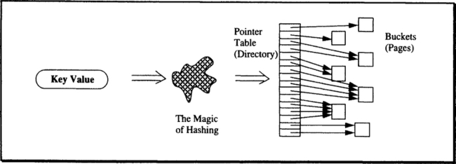
Based on these definitions, let us now explain the key steps of extendible hashing by means of an example. For simplicity, the hashing function is cut short: the binary representation of the numerical key value is used as the bit string S. The example starts at a moment when the directory has 23 = 8 entries (see Figure 15.15).

The convention adopted for addressing the directory of 2d entries is the following: given the bit pattern S, take the d rightmost bits interpreted as a binary integer and examine the corresponding directory entry. This is why the directory always contains 2d entries, with integer d. Since by definition each entry contains a valid pointer, each hashed key will be routed to a bucket page where either the corresponding tuple is found or the decision can be made that the value does not exist. Figure 15.15 contains the example for key value 37. Now try the same thing with 41. Its binary representation is 1010012; thus the three low-value binary digits to consider are 001, which leads to entry 1, pointing to a bucket with key values 1 and 25. Therefore, no tuple with key value 41 is stored in the file.
Looking at Figure 15.15 a bit closer reveals some more detail. There is a number associated with each bucket, and there are some buckets with two pointers going to them. With a larger directory, there could be more pointers to the same bucket, but the number of pointers directed at any bucket will always be a power of two; the reasons for that will soon become obvious. The number going with each bucket is called local depth (as opposed to d, the global depth). Let bj denote the local depth of an arbitrary bucket j, and let #pj be the number of pointers directed at j from the directory (1 ≤ #pj ≤ d). Then the following invariance holds: bj = d – #pj + 1.
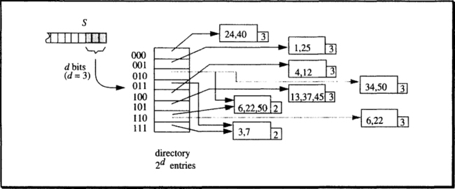
A more intuitive interpretation is the following: the local depth says how many bits of S are actually needed to decide that the key value must be in that bucket. Because d is its maximum value, the local depth can never be larger than the global depth. But it may well be lower, which is the case for all buckets to which more than one pointer is directed. Consider, for example, the entries with indexes 2 and 6. Their binary representations are 0102 and 1102, respectively. The bucket both entries point to contains 50, which is characterized by 010; as well as 22, the last bits of which are 110. Effectively, then, this bucket holds all keys with 10 as the last 2 bits; whether the next bit is 0 or 1 is irrelevant. This is what “local depth = 2” refers to.
How does update work with extendible hashing? The normal case is straightforward. Assume a new tuple with key value 24 is to be stored. Its three relevant bits are 000. First, a normal retrieval is done. The bucket pointed to by entry 0 only contains key value 40; thus, 24 is not a duplicate. Since there is enough space in the bucket, the tuple with key value 24 is stored, and the insert operation is completed.
The next case is demonstrated by assuming that a tuple with key value 34 is inserted. Its three index bits are 010; that is, it is directed to a bucket with local depth = 2. Because this bucket cannot accommodate another tuple, a file extension must be performed—remember that there are no overflow buckets. Since the local depth of the affected page is smaller than the global depth, this amounts to a simple bucket split, as it is illustrated in Figure 15.16.
What is key here is that two pointers are pointing to the overflowing bucket (or 2n, in general). Since this routes too many tuples to the bucket, another bucket is installed, and the tuples are distributed over these two buckets. To distinguish between the two buckets after the split, one more bit from S is considered; note that the local depth of the overflowing bucket is smaller than the global one. As a result, the local depth of each of the buckets resulting from the split is one higher than the local depth of the bucket before the split. Accordingly, the criterion for deciding which tuple goes to which bucket is different from the one used in B-tree splits. Consider Figure 15.16: the two buckets resulting from the split will have one pointer each (shown as shaded arrows), corresponding to the directory entries 0102 and 1102, respectively. Therefore, the tuples must be assigned to the buckets by the following rule: let b1 and b2 be the buckets resulting from a split and i1 and i2 be the indices of the directory entries holding the pointers to b1 and b2. Then all tuples from the old bucket (including the new one that caused the split) whose index bits are equal to i1 are assigned to b1. The index bits of the others will necessarily be equal to i2; they therefore go to b2.
The locking and logging issues are straightforward for the operations described so far. Locks are acquired for the tuples, and the required access paths are protected by semaphores. For recovery purposes, the same physiological logging design is used as was described for B-trees. So the insert (or delete operation is logged in the beginning, and all the subsequent page maintenance operations are logged physically for REDO (note that the directory is mapped onto pages, too).
In case of a bucket split as illustrated in Figure 15.16, there is a potential for semaphore deadlock. Assume transaction T1 comes via directory entry 0102 to the page before the split, protecting its path with exclusive semaphores. Transaction T2 comes via entry 1102, trying to insert into the same page. Now T2 waits for a semaphore on the page, whereas T1 waits for a semaphore on directory entry 1102 to perform the split. In order to avoid such deadlocks, there must be additional rules about when a transaction must not wait for a semaphore. We will not discuss that issue here.
This gives an idea of how the file can grow, given a directory with 2d entries. But now assume a tuple with key value 61 is to be inserted. Its index bits are 101, the corresponding bucket has local depth = 3, and it is full. Another bit cannot be appended to the left to distinguish two buckets after a split, because the directory itself is addressed by only three bits. Before the bucket can be split, therefore, a larger directory must be built. Its number of entries must be a power of two, so its current size is simply doubled. This implies that the global depth d is increased by 1 (the next bit from S left of the ones currently used is included). As a consequence, all buckets have a local depth smaller than the (new) global one and, therefore, the split algorithm can be applied.
This whole procedure is illustrated in Figure 15.17; its left-hand side is a cleaned-up version of Figure 15.16.
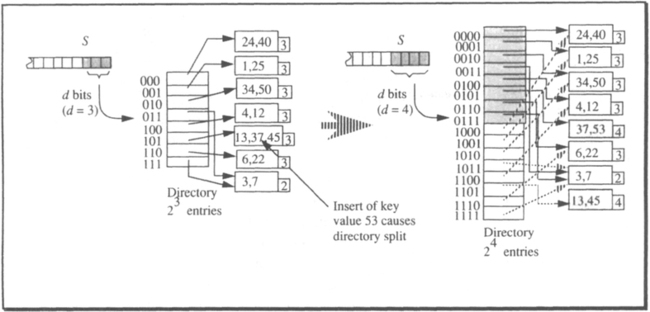
The question of how to double the directory and what to put into the new entries is simple. Since the bits from S are included with increasing exponents, an entry with the old number xyz will now turn into two entries with number Oxyz and lxyz. Of course, all key values that up to now had index bits xyz will remain unchanged; that is, for locating them, the string xyz is sufficient. Therefore, both new entries will contain the same pointer, the one that was stored in entry xyz in the old directory. Since this consideration applies to all entries, doubling the directory means the following: a copy of the old directory is placed directly behind its highest entry. The resulting table with twice the number of entries is the new directory.16 Note that when doubling the directory, the whole directory must be locked exclusively until the operation is completed. This is not comparable to the situation of a root split in a B-tree. Whereas even in a large B-tree at most five to six pages are modified during an insert causing a root split, doubling the directory of an extendible hashing file with 106 pages means that some 6 MB must be copied explicitly—potentially causing substantial I/O along the way.
In Figure 15.17, the old directory portion is shaded; the new one is not. The copied pointers are indicated by shaded arrows. The figure also contains the result of the bucket split that originally triggered the directory split. The resulting buckets are represented by shaded boxes; of course, after the bucket split is completed, both buckets have the new global depth as their local depth.
The performance of the extendible hashing scheme is fairly easy to estimate. For simplicity, let us concentrate on retrieval operations. The additional cost for inserts only depends on the frequency of splits, which in turn is influenced by how much the file grows compared to the original space allocation. Because the frequency of directory splits decreases exponentially as the file grows, this should not be a cost factor.
There are always two steps for retrieving a tuple (not counting the hash function): first, access the directory to find the bucket pointer; then read the bucket page. As long as the directory completely fits into main memory (into the buffer), each retrieval is one page access—the minimum cost. Assuming 4 bytes per entry and 4 KB pages, then with a 1 MB buffer space for the directory, a 1 GB extendible hash file can be maintained, allowing for one-access associative retrieval.
This sounds pretty attractive, but there are some hidden problems that will surface as soon as a real implementation is considered. We will list just a few of them. The estimate yielding the 1 GB file is based on the assumption that each pointer in the directory goes to a different bucket. Of course, this is only the case if the index bits of the key values in the file are uniformly distributed. If the hash function does not produce a uniformly distributed bit pattern, those parts of the directory corresponding to the more frequent bit patterns will experience a higher frequency of splits. This, in turn, means the directory will be larger than it had to be to address the given number of buckets. And note that the directory doubles each time one bucket is about to exceed the global depth. It does not help if the local depth of the others is way below that value. In other words, for hash value distributions with a noticeable bias, there will quickly be a directory that is relatively large compared to the number of buckets it manages. Once the bucket entries can no longer be kept in buffer, additional page accesses are required for reading the needed portion of the directory. In the worst case, each tuple access requires two page accesses. This is worse than static hashing, and it is not much better than B-tree performance (if at all), considering that the top two levels of a B-tree can be kept in buffer. The question, then, of whether the additional flexibility provided by extendible hashing is worth the effort from a performance perspective critically depends on the quality of the hash function.
Another problem is shrinking an extendible hash file. If a bucket becomes empty, its pointer can be redirected, but deciding whether or not the directory can be cut in half requires additional bookkeeping. It should also be clear that each structural change of the directory is a complex operation, rendering the file inaccessible for quite some time.
And, finally, there is the question of how to map the directory onto disk. A small directory fitting into main memory is not a problem, but what about large ones that have to be paged just like any other data structure? The speed of the algorithm is due to the fact that, based on the index bits, the bucket pointer can be located at almost no cost. If this is to translate to a disk-based directory, then the directory must at any point in time be stored in consecutive pages. If one does not want to allocate space for the largest directory possible, what happens at a directory split?
15.6.2 The Grid File
The grid access method addresses a functional limitation inherent in all the techniques described so far: symmetric access via multiple attributes. Consider the B-tree algorithm and assume that a relation is to be associatively accessed using the values of two attributes, A and B. The queries can be of any of the following types: (p1(A,B)), (p1(A) con p2(B)), (p1(A)), (p2(B)). Here pi denotes predicates defined over the respective attributes, and con is a logical connector, such as and, or, exor.
There are two possibilities for supporting such B-trees queries:
Two B-trees. A B-tree is created for each of the two attributes, and the (partial) predicate referring to A is evaluated using the tree on A; the same applies to the (partial) predicate on B. This produces two partial result lists with TIDs that then have to be merged or intersected, depending on the type of con.
One B-tree. A B-tree is created for the concatenated attribute A || B or B || A. The query predicates are then evaluated using the value combinations in the tree.
Detailed analysis reveals that neither variant works for all query types. The first one has the problem of employing two access paths. This is substantially more expensive than using just one adequate access path; the necessity of maintaining partial result lists and storing them for final processing further adds to the complexity of this solution. But even if all this were acceptable, it is clear that a query with a simple predicate like (A > B) cannot be supported by having two separate B-trees.
Creating a B-tree over the concatenation of both attributes reduces the cost for query processing in some cases, but there are also query types that do not benefit from such an access path. The predicate (A > B), and all variations thereof, is one example. But there are even more trivial cases. Assume the B-tree has been created for A || B; this tree can then be used for answering the query (A < const), but it is useless for (B < const).
Maintaining separate trees for all types of attribute combinations in all permutations solves some of the retrieval problems, but it adds unacceptable costs to the update operations. Considering the arguments already given, it is obvious that for n attributes, virtually all n! attribute concatenations would have to be turned into a B-tree in order to get symmetric behavior with respect to range queries on arbitrary subsets; this is certainly not a reasonable scheme.
What is needed, then, is an access path to allow efficient associative access in an unbiased fashion, based on n attributes with queries of the types shown for the special case of two attributes. For simplicity, all the following presentations are also restricted to two attributes, but a generalization to n attributes is not difficult.
The grid file is one of the most thoroughly investigated access methods for symmetric multi-attribute access in large files. The best way to introduce the basic idea is to use the metaphor of a point set in a plane. Each attribute is an axis in a euclidian space. The tuples have well-defined values in the search attributes A and B; thus, each tuple corresponds to the point in the plane having the tuple’s attribute values as its coordinates. This is illustrated in Figure 15.18.

There are two evident reasons why such a “tuple space” cannot be used directly for storing the tuples: first, it has at least two dimensions, whereas the page address space is one-dimensional; second, the n-dimensional tuple space has clusters as well as unused regions, whereas the utilization of the storage space should be uniformly high. But as Figure 15.18 suggests, the arrangement of the points in the plane (sticking to the two-dimensional example) contains enough information to decide for which regions (subspaces) storage space must be allocated, where the density of tuples is high, where no tuples are, and so on.
Given the point set shown at the left-hand side of Figure 15.19, and given pages which can hold up to three tuples, we can replace the plane with a two-dimensional array of pointers, as shown on the right-hand side. Each of the four cells contains exactly one pointer to a page where the actual tuples are stored; the shaded points in the cells merely indicate which of the tuples of the point set on the left are in the pages to which the pointers refer.
The key point of the grid file concept is the following: as Figure 15.18 shows, the subspaces called cells are not of equal size in terms of the attribute dimensions, although each of them contains one page pointer. The criterion for determining the cell sizes is the number of points in the cell. In other words, the limits between neighboring cells along each dimension are adjusted such that biases in the value distribution are compensated. In value ranges with high tuple frequencies, the sides of the cells are smaller; ranges with fewer tuples allow for larger cells.
Since the value space is divided by parallel planes to the axes, the dividing points for each dimension can be stored separately in an array called scale. Each scale corresponds to one attribute dimension, and it contains the values of that attribute where a dividing plane cuts through the value space, thus creating the cells. It is assumed that each scale array contains the dividing points in ascending order; that is, the larger the index, the larger the attribute value. The data structures required for the two-dimensional case can be declared as follows:
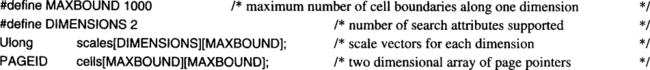
Note that these declarations serve only the purpose of illustrating the functional principles of the grid file. In a real implementation, scales would probably not be defined as a two-dimensional array, because the number of cell boundaries along the different attribute-dimensions may vary widely. The array of page pointers cells cannot be kept in main memory for large files. Consequently, there must be some way of mapping the array onto pages; this is discussed later in this subsection. (See also the remarks on maintaining the directory for extendible hashing in Subsection 15.6.1.) By the way, the cell array is often referred to as the directory of a grid file.
Given these data structures, it is easy to explain how retrieval works with a grid file. Let us start with an exact-match query, which is also referred to as point search when talking about multi-attribute search structures. A point query has a search predicate of the type (A = c1 and B = c2). In terms of the point set metaphor, this means that the tuple corresponding to the point in the plane with the coordinates (c1,c2) has to be retrieved. The basic steps are illustrated in the piece of code that follows (note that all concurrency control on the scales, index arrays, and cells is omitted).
Thanks to the simplifications explained previously, the code skeleton for retrieval is surprisingly small. It stops in a situation comparable to the moment when the right leaf node in a B-tree is located: the page accessed through bufferfix is the one where the tuple with the specified search must be stored, if it exists. Locating the actual tuple requires a subsequent search in the page.
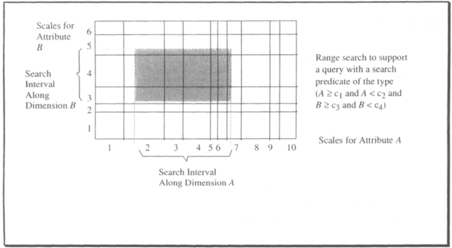
The generalization from point search to interval search along arbitrary dimensions is obvious. Search intervals are defined by specifying the coordinate ranges along each dimension, rather than single coordinate values. Accordingly, for each dimension, a cell index range, rather than a single index, is determined from scales. And finally, cells is accessed with all possible combinations of the cell indexes within the relevant ranges. This yields a set of page numbers completely covering the subspace defined by the range query. It is illustrated in Figure 15.19. The indexes of the two scale vectors are explicitly shown in the figure, for ease of reference.

Given the specified search ranges, the scale for attribute-dimension A says that cells must be accessed with the first index varying between 2 and 7; the scale for B prescribes an index range between 3 and 5. Therefore, the access to all tuples potentially falling into the search rectangle requires the following actions:

Because the whole business of updating a grid file—especially inserting new tuples—is fairly complex, we will only explain the principles involved. The key issues are that grid files are dynamic (pages are allocated and freed as needed) and that the subdivison of the scales into value ranges for determining the cell boundaries has to be dynamic. In other words, there is no prearranged cell structure (this would make things very easy); rather, the boundaries of the cells are adjusted according to the value distributions of the tuples in the file. As an example, assume more tuples are inserted into the scenario of Figure 15.18. These tuples are given names, for ease of reference. Figure 15.20 illustrates the aspects of updating a grid file.
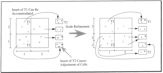
As always, insertion begins with a retrieval operation (a point search for a grid file) to locate the page where the tuple to be inserted has to go. If the page can accommodate the tuple, the tuple is stored there, and no other data structures are affected. In the example, this is the case for tuple t1. If, however, the page is full, its contents have to be distributed across two pages, and the addressing scheme has to be adjusted accordingly. This is similar to how extendible hashing works.
The directory of a grid file has a page pointer for each subspace, the limits of which are determined by the scales. If a page has to be split, two pointers are needed; that is, the subspace entry in the directory must also be split. As Figure 15.20 shows, the critical subspace with cell indexes (1,1) is split along the vertical dimension (shaded line). As a consequence, all cell entries with indexes (*,1) turn into two entries with indexes (*,1) and (*,2). Except for the split cell, all other cell contents are simply copied; this is also shown in the illustration.
Along the dimension that was chosen for the split, all index values above the point of split for existing cells must be increased by one. This requires special techniques for efficiently maintaining the multidimensional directory, discussion of which is beyond the scope of this short introduction.
If a page becomes empty, its pointer in the directory can be redirected to a neighboring page. Neighborhood is defined along any of the dimensions. If an entire subspace along one dimension becomes empty, no entries for it are needed in the directory, and the scale for that dimension can be reduced accordingly. This is the inverse of the process shown previously.
There are a number of difficult problems associated with an efficient implementation of the grid file scheme for a general-purpose transaction system. Splitting is much more complex than shown in our example. The first question concerns which dimension to split along in case of a page overflow. There are different options, depending on how much information about the state of neighboring cells is included. The really tricky issue, however, is how to maintain the (large) directory on disk efficiently. As was demonstrated, the directory is a dynamic, n-dimensional array, and each split operation means that (n – l)-dimensional subarrays are inserted at the split position. Such an operation should not imply a total reorganization of the whole directory. Furthermore, it would be desirable to store the pages associated with neighboring subspaces within a narrow address range. Such a clustering should be maintained under update.
And then, of course, there is the problem of synchronization on a grid file. Which locking protocols are needed for the scales, the directories, and so forth? Is the value locking technique used for B-trees applicable?
Assuming that all these problems can be solved, grid files yield a constant cost of two page accesses for a single-point retrieval. This assumes that the scales can be kept in buffer which is reasonable because they normally comprise just a few KB. Then, one access is required to find the directory page for the subspace in which the point lies, and one access goes to the data page. The performance characteristics and the functional principle are very similar to the extendible hashing scheme. One difference is that extendible hashing is one-dimensional, whereas the grid file supports multidimensional access. Another difference is that extendible hashing relies on a hashing function (hence the name) to produce uniform access frequencies to all directory entries; the grid file employs the scales for the same purpose. And the last, but important, difference is that the directory of an extendible hashing file is much simpler to maintain (and therefore to implement) than the multidimensional directory of the grid file.
15.6.3 Holey Brick B-Trees
Holey brick B-trees (hB-trees) address the same problem as grid files: symmetric multi-attribute search on large files. Just like grid files, they support both exact-match queries and range searches along arbitrary subsets of the attributes on which the search structure is defined. But whereas grid files rely on a multidimensional array that actually resembles the structure of the search space, hB-trees (as their name suggests) are much more akin to B-trees as they have been described in this chapter. It makes an interesting exercise to compare these two radically different approaches to the same problem. But let us first illustrate the basic idea behind hB-trees.17
The name holey brick B-trees intuitively conveys its idea. Each node in the tree corresponds to a rectangular k-dimensional subspace of the total search space (assuming the search structure has been defined on k attributes of the file). These subspaces are referred to as bricks. In contrast to similar search structures, where this correspondence is strict, a node in an hB-tree generally describes a brick from which smaller bricks may have been removed. This means that the bricks into which the search space is decomposed can have “holes”—hence the name of the access path structure. Like a B-tree, an hB-tree grows from the leaves to the root. The leaves contain the data, whereas the higher levels consist of index nodes.
When speaking of hB-trees, we have to distinguish carefully between two types of tree structures. One is the overall structure of the hB-tree; that is, the way its index and data nodes are tied together. This is taken from the K-D-B-tree (K-D stands for k-dimensional), a B-tree generalization for k attributes. This method was introduced by Robinson [1984], and its principle will become clear during the following description. The second type of tree structure is the k-d-tree [Bentley 1975], which is used to internally organize the entries of the index nodes in an hB-tree. Let us first sketch the ideas behind a k-d-tree.
A k-d-tree is a binary tree that structures the search via k different attributes. Its principle is illustrated in Figure 15.21. A node in a k-d-tree represents an attribute value. If the search key value is less than the node value, search proceeds to the left, otherwise it proceeds to the right.18 So far, this is exactly how a binary tree works.

However, in a conventional binary tree, each node represents a value of the same attribute; in a k-d-tree, on the other hand, subsequent nodes along a search path can represent values of different attributes. The simplest rule to cope with this is to use the k attributes in a fixed order. Therefore, if the tree is defined on k = 3 attributes (a, b and c), then the root node contains a value of a, its two successors contain values of b, their successors contain c values, then comes a again, and so forth. This is simple but potentially inefficient, because at a certain level it forces the use of an attribute even if the subspace considered at that level need not be partitioned along that dimension. For example, in Figure 15.21, subspaces C and D are defined by values of b only; attribute a is not relevant for them. Thus, a more sophisticated scheme for the k-d-tree permits using along any search path, that attribute for the next node that yields the most efficient partitioning of the remaining subspace. As Figure 15.21 shows, this may result in the same attribute being used repeatedly. Since with that convention, a node’s distance from the root allows no conclusion as to which attribute the node represents, another scheme is sometimes used: each node except for the value must also carry an identifier of the attribute to which it belongs. In what follows, that second scheme is assumed.
As shown in Figure 15.22, the representation of holey bricks by generalizing the k-d-tree technique is straightforward. The conventional search structure is based on the assumption that each node defines a partitioning of the subspace it represents along one dimension, and all dependent nodes further subdivide that partition; here, however, multiple nodes can point to the same partition. When you look at Figure 15.22, the consequences become obvious: in a conventional k-d-tree, the left pointer of the node representing a1 would have to point to a separate subspace, thus partitioning the right-hand region of the search space. However, since this portion of the region, together with the left-hand part of the search space, establishes the subspace B, from which the hole A has been removed, the pointer refers to B, too.

So much for the introduction of the data structures used in the index nodes of an hB-tree. Let us now consider overall organization of an hB-tree. This is where the need for holey bricks comes in. As mentioned, the structure of an hB-tree is similar to a K-D-B-tree. K-D-B-trees are much like B-trees in that they are balanced, the data is in the leaves only, and so on. But while each index node in a B-tree describes the partitioning of a region of a one-dimensional search space into disjoint intervals, an index node in a K-D-B-tree describes the partitioning of a region of a k-dimensional search space into k-dimensional subspaces. For each subspace, a lower-level index node is pointed to, describing the partitioning of that subspace into even finer granules, down to the leaf level.
Up to this point, we have described exactly what the hB-tree does. The difference lies in the techniques used to maintain the tree structure during update. When an index node has to be split in a K-D-B-tree, one attribute (dimension) is picked, along which the subspace represented by that node is divided into two. In other words, the old subspace is completely partitioned along a (k – 1)-dimensional hyperplane. There are two problems with this approach:
Uneven partitioning. Depending on the location of the tuples in k-space, it may not be possible to find a single-dimension partitioning that yields even distribution of the entries across the two nodes resulting from the split.
Cascading spilts. B-trees have the property that splits are always propagated bottom-up: as a result of a node split, its parent node may have to be split. But splitting an index node has no impact on any of its child nodes. In K-D-B-trees, however, the method of splitting along one dimension causes splits to cascade down the tree to child nodes (and maybe to their children) to adjust for the new setting of subspace boundaries.
The hB-tree uses a different split strategy. It allows a node to be split along more than one dimension in order to avoid both of the problems just mentioned. As a consequence, however, one must be able to cope with holes in the subspaces represented by the index nodes. Since the representation of holey bricks is based on multiple nodes pointing to the same successor (see Figure 15.22), this may result in one index node having more than one parent. Strictly speaking, then, we would have to talk about “hB-DAGs,” but since we will not go into any detail with respect to mutiple parents, the notion of trees is used throughout this section.
To understand the following description of the operations on hB-trees, we have to appreciate the global layout of this search structure, which is depicted in Figure 15.23. The leaves of the k-d-trees in the index nodes point to lower-level nodes in the tree. More than one pointer can reference the same successor node, and these multiple references of the same lower-level node can come from different higher-level index nodes. In each k-d-tree, holes that have been extracted from the region described by the node are tagged (* in the figure). The data nodes also contain k-d-trees to guide the local search, but here the leaves are the actual tuples (or pointers to the tuples, for that matter). Note that in the general case, a leaf of a data node k-d-tree can represent many tuples, namely all those falling into the subspace denoted by that node in the k-d-tree.

Searching in an hB-tree is straightforward. Let us briefly consider the two types of access operations supported by such a search structure.
Exact-match query. The k attributes of the tuple(s) to be retrieved must be equal to the values of the k-vector specified for the search operation. Starting at the root, the k-d-tree is used in its standard way. Depending on which attribute the k-d-tree node represents, one compares the respective search value and proceeds along the vector that belongs to the “=” case. This produces a pointer to a lower-level node, which is processed in the same way, and finally one gets to the data node with the qualified tuple.
Range query. This requires following many search paths in parallel. Consider a k-d-tree node pertaining to attribute a. If the value it represents is larger than the upper bound of the range in that dimension (or smaller than the lower bound), then one need only follow the left (or right) pointer. Otherwise, if valid data lies in both directions, both pointers must be followed. The same argument applies recursively down to the data nodes.
Update operations follow the same general logic as B-trees; this is explained by considering the insert of a new tuple. First, an exact-match query is performed to determine the insert location. If the tuple fits into the data page, the insert is complete; no structural modifications are necessary.
The specific properties of an hB-tree become relevant when a node split is necessary. For brevity, we do not discuss all the variants and special situations that have to be considered. Rather, we focus on some typical scenarios to demonstrate the principles of splitting nodes that contain k-d-trees describing holey bricks.
At the core of the split algorithm lies the observation that it is always possible to achieve a worst-case split ratio of 1:2, no matter what the value of k, provided the split can involve more than one attribute.19 When a page needs to be split, therefore, one first checks to see if a split at the current root of the node’s k-d-tree would partition the entries in the page in a ratio of 1:2 or better. If that is the case, the node is split at the root. The left subtree forms one new node, the right sub-tree the other one. If the old node (before the split) represented a complete brick (no holes in it), then there was just one reference to it from an index node. In that case, the old root node must be propagated up to the index node to augment its k-d-tree. If, however, the old node already had holes, then the split may not require any key values to be propagated up the hierarchy; only the adjustment of some pointers is necessary (have them point to the right sub-tree in the new page, rather than in the old one).
If the root node does not achieve the 1:2 split ratio, there must be one sub-tree accounting for more than two-thirds of the entries in the node. Going down this sub-tree produces the first of two possible outcomes (the second will be considered shortly).
Split at lower sub-tree. In the large sub-tree, a node is found, one of whose sub-trees accounts for less than two-thirds and more than one-third of the entries. Then the k-d-tree, and thereby the hB-tree node, is split at this point. This is illustrated in Figure 15.24.
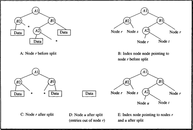
The node to be split (node r) represents a holey brick. Splitting at the node for attribute b1 gives the required split ratio, so the left sub-tree of that node is removed. Since it contains only one portion of data, the new node (node u) can, for the moment, do without any local k-d-tree. The removal of the sub-tree is marked in node u by the tag representing a hole in the appropriate branch. In other words, the split has caused the brick described by node r to get a new (bigger) hole. The example also illustrates that in cases where the discriminating attribute’s values are already present at higher levels, a split may result in mere pointer adjustments in the index.
Note also that the local k-d-trees resulting from the split are generally reduced to the minimum number of nodes required to represent the remaining region in space. This may also result in the removal of hole references (see node u).
Split at leaf. If no sub-tree with the required property is found, then one of the leaves must account for more than two-thirds of the entries; this can only occur in data nodes. In that case, the data in that leaf must be redistributed. According to the split ratio property mentioned earlier, it is always possible to determine a hole lying at a corner of that subspace, such that the ratio of entries in the hole and in the remaining brick is 1:2 or better. The attribute values defining that corner must be propagated up to the index level. An example in two dimensions is shown in Figure 15.25.

The tree structure of the data node and its index node is assumed to be the same as in the previous example. However, we now consider the case in which no sub-tree accounts for a number of entries that lie between one-third and two-thirds of the entries in the page. Assume the data portion in the high-value branch of b1 has more than two-thirds of the entries. This brick must be partitioned, and, as we have seen, there is always a corner hole to remove from the brick such that both the removed part and the remaining part of the node to be split hold between one-third and two-thirds of the entries. Figure 15.25 shows the result of the split, assuming that the removed part was actually sliced off the large subspace along dimension a at point a3. As in the previous scenario, the removed data portion goes to a new page (node u); being the only portion in that node, it needs no k-d-tree for the moment. The new node in the k-d-tree of node r is propagated up to the index node.
As an aside, assuming a1 < a2 < a3 and b1 < b2, we find that the holey brick described by node r now has become holey to the degree that it is noncontiguous. In other words, the holes separate the remaining parts of the subspace that actually contain data maintained in that node.
To keep this discussion short, we do not elaborate on exactly how nodes resulting from a split are propagated up to the index nodes; what happens in case of multiple parents; and so forth. The material presented so far should be sufficient to convey the idea.
The hB-tree structure is interesting for a number of reasons. First, it is a generalization of the well-established B-tree access path, and some of its organizational principles can be applied without any changes. It guarantees a fixed minimum node utilization, even with the worst-case data distribution. This is its major difference from the grid file, for example, which works well only if the data points are evenly distributed in the search space, and which can deteriorate badly if that is not the case. A consequence of the one-third minimum node occupancy is a limit on the height of the hB-tree. For a given file, the hB-tree should come out only slightly higher than a B-tree. This is partly due to the lower (minimum) node utilization and partly due to the fact that the number of entries per node is lower for an hB-tree in the first place, because information about k attributes (rather than one attribute) has to be maintained. Analytic models show that an hB-tree with just one dimension has a performance comparable to that of a B-tree.
A consideration of synchronization and recovery techniques for hB-trees is beyond the scope of this discussion. Even these brief explanations, however, should convey the fact that this is an altogether different story.
15.7 Summary
Associative accesss paths have to serve two basic functional requirements: first, exact-match queries have to retrieve all tuples whose value in a given attribute (or set of attributes) is equal to a specified search key value. Second, range queries must be supported to retrieve all tuples whose attribute values are elements of a specified search interval (range). Support of such queries basically implies the possibility to access tuples in sorted order of the attributes defining the boundaries of the query range.
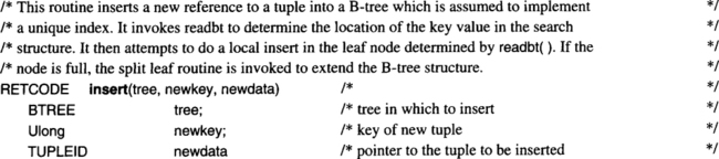
Exact-match queries are supported by hashing. The functional principle can be characterized as follows: upon tuple insert, take the value of the attribute that will subsequently be used for exact-match queries (typically this is the primary key) and transform it (by arithmetic computations) into a relative page number of the file where the tuple is to be stored. For retrieval, the same procedure is applied, too, so the page to be read from disk can be directly computed from the attribute value. Complications such as skewed value distributions in the relation and collisions resulting from that notwithstanding, hashing provides single-page access behavior, which is the absolute minimum for random single-tuple access for the architecture assumed in this book. Whenever very fast random access to single tuples via the primary key (think of account numbers, credit card numbers, and so on) is the dominating performance criterion, hash-based access is an option. It has serious drawbacks, though. Range queries are not supported, exact-match queries via nonunique attributes are possible only within narrow limits, and the size of the relation must be stable over time (and known in advance).
Apart from hashing, which lives in some sort of an ecological niche, the dominating species among the associative access paths in today’s databases is the B-tree. It is a multi-way search tree with a number of very attractive features. First, it meets all the functional requirements mentioned. Second, its performance characteristics are predictable precisely, because the tree is at any point in time perfectly balanced in terms of the number of nodes that have to be visited upon retrieval from the root to any leaf. Its absolute performance is very good, depending of course, on a number of application-dependent parameters and design options. Roughly speaking, a random single-tuple access via a B-tree requires between (H – 3) and (H – 2) I/O operations, where H is the height of the tree, which—for the fast majority of applications—ranges between 4 and 5. For range queries and sequential retrieval in sorted order, the overhead incurred by the tree structure is much smaller. If the B-tree is used to implement a secondary index via a nonunique attribute, the performance characteristics are almost the same.
Since the B-tree is ubiquitous in databases, it is an extremely well-investigated data structure. There are numerous designs aimed at optimizing its performance with respect to concurrent transactions reading and updating data via the same B-tree, and at the same time guaranteeing isolated execution for each transaction using the tree. These protocols get fairly complicated, because they have to make clever use of the semantics of the tree structure and its operations. It is instructive to study both the synchronization and the recovery protocols, because they provide isolation without being serializable in the classical sense.
Mighty as the B-tree may be, there are applications that require more than it can provide. Typical examples are symmetric multi-attribute search operations and retrieval operations that refer to spatial criteria such as neighborhood, overlap, and so on. Once applications in that area are important enough to justify the implementation of dedicated database functions, new associative access paths such as grid files, hB-trees, and others may become relevant. A similar observation holds for access structures supporting complex objects that are typical of object-oriented databases. It is interesting to observe, though, that the most promising of these “new” search structures more often than not are close relatives of the B-tree.
15.8 Historical Notes20
The history of access paths, like many other aspects of transaction systems, is a story of rediscovering the same few principles over and again. Both fundamental techniques—key transformation and key comparison—have been in use in many areas of human activity for at least 200 years, probably much longer than that.
Indexing is ubiquitous. Since it requires some kind of alphabet for which a sort order can be defined, preliterate societies most likely had little to do with it. After that, however, the idea is applied in many guises. Large libraries, for example, use multi-level indexing. There is an index for the different rooms, one for the shelves in each room, and one for the boards in one shelf. The boards represent the leaf level, where a search in an ordered set has to be performed.
Another application—one that is is not so old—is phone books. Of course, they essentially have a one-level index; here you are literally operating at the leaf level. But phone books do key compression in much the same way described in this chapter. (Look at the upper-left and upper-right corners of a page and see what kind of reference key is printed there.)
Hashing bears an interesting resemblance to the way the human memory works (or pretends to work). Many techniques for improving the capabilities of one’s memory (especially the quality of recall) are based on the trick of associating the information to be remembered with something else, something familiar; these are called mnemonic devices. Upon recall, the access to the familiar thing is easy (page number), and associated with it comes the information requested. As in the technical environment, the performance of such techniques critically depends on the quality of the “hash function.”
Now let us close in on the much narrower domain of databases and transaction systems. The descriptions of many of the basic algorithms can be found in one of the classics of computer science, Knuth’s The Art of Computer Programming [1973]. Understandably, however, this work gives no consideration to the issues related to maintaining such structures on external storage, and to synchronization and recovery.
One of the earliest attempts to implement multi-level indexes was the index-sequential access method (ISAM) in the OS/360 operating system. The original version was far from the flexibility of B-trees, though, because the index structure was bound to the geometry of magnetic disks. There was a master index pointing to directories, each directory had an index pointing to tracks, and each track had an index pointing to records. It actually was not as simple as that, but this is the basic idea.
The elaboration of what finally came to be known as B-trees was carried out in the mid-1960s in different places and, of course, in isolation. The database management system ADABAS, the development of which started at about that time, from the very beginning made massive use of dynamic multi-level indexes. As a matter of fact, each ADABAS database is something like a “supertree,” in that all existing access paths are linked into a higher-level tree, with the catalog on top of all that. Probably for confidentiality reasons, there is no precise description of which algorithms are used, how locking and recovery are done, and so on.
The first concise paper—and the most famous one—about the B-tree is by Bayer and McCreight [1972]. Most of the subsequent literature is based on the concepts presented there, although many of the contemporary implementations were done without the implementors having seen them.
Over the years, the ISAM access method was made more and more device independent and gradually turned into VSAM, which is (among others) a full-blown implementation of B-trees, with key compression and everything else. As part of the operating system, VSAM does not know about transactions. The reader should by now be able to appreciate what it means to keep a data structure consistent after crashes without the benefits of a log, a recovery manager, and so on. VSAM has its very own mechanisms for fault tolerance, which have not been described in this book. Fundamentally, they are an elaborate version of careful replacement.
The development of relational databases brought about another round of B-tree implementations. The system implementation on the large scale is fairly well documented [Astrahan et al. 1981; Haderle and Jackson 1984; Tandem Database Group 1987; Stonebraker et al. 1976]. Yet the details of how the access paths actually work have never been published.
There have been several general expositions of B-trees. The best-known is the survey article by Comer [1979]. Textbooks on file structures usually have an explanation of B-trees. Many of the performance formulas worked out in this chapter, for instance, can also be found in [Salzberg 1988]. Salzberg’s book also covers linear hashing [Litwin 1980], bounded extendible hashing [Lomet 1983], grid files, hB-trees, an optical disk access method, external sorting, and relational joins.
Papers suggesting ways to improve the general B-tree algorithms (to increase fan-out, for example) have also been published. The handling of variable-length keys and use of key compression within B-tree nodes was presented by Bayer and Unterauer [1977] and Lomet [1979]. The use of multi-page nodes for leaves is investigated in Lomet [1988] and Litwin [1987]. Having larger leaf nodes can decrease the number of disk accesses. Using partial expansions [Lomet 1987] can increase the average space utilization in leaves, also improving on the number of disk accesses. Having larger index nodes [Lomet 1981; 1983] can increase the fan-out.
In the late 1970s and in the 1980s, a number of academic researchers published papers on concurrency in access methods. These papers, in general, do not consider such system issues as whether I/Os occur while locks are held, what happens on system failure, and so forth. They concentrate on making search correct while insertions and deletions are in progress. Usually there is an implicit assumption that system failures do not occur. Some of the earlier papers on concurrency in tree structures include work by Bayer and Schkolnick [1977] which contains the safe node method used in this chapter, [Lehman and Yao 1981; Ellis 1980; Kung 1980; Kwong 1982; Mandber 1982; and Ford 1984]. The work reported by Sagiv [1986] extends the work of Lehman and Yao to include restructuring. The paper by Shasha and Goodman [1988] gives an integrated description of the principles involved in most of the concurrency algorithms.
Two recent papers [Srinivasan 1991; Johnson 1991] analyze the performance of concurrent B-tree algorithms. Both conclude that the Lehman-Yao method performs best.
In contrast, most of the work on actual implementations of B-trees in commercial systems has never been published. For example, Mike Blasgen, Andrea Borr, and Franco Putzolu have written several B-tree implementations and may very possibly know more than anybody else about how it must be done, but they have never written papers about it.
Implementors of commercial systems have had to consider system failure and recovery, the length of time locks are held (whether I/O or network communication occurs during the time locks are held), lock granularity and lock mode, and the complications of key-range searching and its susceptibilty to the phantom anomaly. These constraints led to a different perspective, which decisively shaped this text but which has been largely invisible to the academic community. Until the papers of Mohan and his colleagues at the Database Technology Institute at IBM’s Almaden Research Lab began to appear, it was not possible for people not active in commercial implementation to gain this perspective.
Mohan and his colleagues have published a series of papers on a design for recovery, access path management, and concurrency control called ARIES. A number of these are cited in the references. In particular, the ARIES/KVL paper [Mohan 1990a] is the basis for the discussion of the tuple-oriented view of B-tree synchronization in Subsection 15.3.4. Other papers dealing with B-trees include ARIES/IM [Mohan and Levine 1989] and Mohan et al. [1990]. These papers are very detailed and are difficult to read, but they are worth the effort.
Hashing has been used in almost every component of operating systems, database systems, compilers, and so forth, from the very beginning. Look, for example, at the sample implementations of a lock manager in Chapter 8 and of a buffer manager in Chapter 13. Every book on elementary data structures describes the use of hashing for implementing content addressability in main memory. These mechanisms have been applied to file organization in many database products and other types of data administration software. Some of the earliest implementations of that type have been bill-of-material processors (BOMPs), which essentially used two access paths: hashing for associative access via the part number, and physical chaining for maintaining the “goes into” relationship. Many of these special-purpose packages have been the precursors of general-purpose database systems (IMS and TOTAL, for example).
But generally, the hashing technique used was static hashing with some kind of collision handling, as described in this chapter. When hashing is used in commercial products, this is likely to be how it is done even though it will require massive reorganization when the data collection grows, and even though many suggestions for dynamic hashing have been made in the literature.
In Subsection 15.5.1, we have seen one such suggestion—extendible hashing—as described in Fagin et al. [1979]. An improvement on this basic design, which prohibits the index from growing too large to be kept in main memory is found in Lomet [1983]. An alternate suggestion is linear hashing [Litwin 1980]. Several suggestions for improving linear hashing can be found Larson [1980; 1982; 1983; 1988].
Concurrency in linear hashing is treated in Ellis [1985], and Mohan discusses both concurrency and recovery Mohan [1990c]. Ellis [1982] covers concurrency in extendible hashing. In spite of all this work, these suggested dynamic hashing schemes have not yet been implemented in any commercial products. This would contribute to the suspicion that B-trees, which do not need massive reorganization and which can handle range queries, have been judged adequate for most applications.
Classical applications in banking, inventory control, flight reservation, and so forth need fast access to one tuple by primary key, and efficient access to a small number of tuples via a secondary key. B-trees do satisfy these requirements with sufficient performance. Nonstandard applications such as computer-aided design, geographic databases, biology databases, process control, and artificial intelligence have other requirements. They may need to cluster records by several attributes. They may deal with complex objects—a part together with all its component parts is a good example. So file organizations supporting value-dependent clustering is certainly needed for systems adequately supporting these applications.
New types of indexes have been proposed, especially for applications dealing with geometric data of some sort. In this chapter we have seen the grid file [Nievergelt, Hinterberger, and Sevcik 1984] and the holey brick tree [Lomet and Salzberg 1990b]. Other promising spatial indexes include the R-tree [Guttman and Stonebreaker 1984] and z-ordering [Orenstein 1984].
Although both Salzberg [1986] and Hinrichs [1985] have proposed concurrency control methods for the grid file, these methods do not treat system failure and are somewhat complicated due to the non-local splitting in grid file systems. Also, as with most published work on concurrency in access methods, other system issues (range locking, I/Os while locks are held) are not addressed. Work is ongoing for implementations of concurrency and recovery for holey brick trees.
The simplest spatial index to implement is the z-ordering method, so this is the one most likely to appear in a database management system. For z-ordering, one merely interleaves the bits of the attributes of the key and then places the interleaved bit string in a B-tree. The already developed concurrency and recovery algorithms for B-trees can then be applied. The question of range locking is interesting, for the spatial (rectangular) ranges do not correspond to the linear ranges of the interleaved key. In fact, how to make such rectangular range queries efficient has been the subject of several papers [Orenstein 1986; 1989].
In addition, there have been suggested temporal indexing systems [Lomet and Salzberg 1989a; 1990a] and indexing systems for object-oriented databases [Bertino 1989; Maier 1986]. Object-oriented systems are in great demand and are not as efficient as one would like, so there is sure to be more activity in this area.
Summarizing then, the B-tree is still ubiquitous. Almost every database management system, even single-user microcomputer DBMSs, has them. For large transaction systems, sophisticated concurrency and recovery methods have been developed. Static hashing is sometimes used, but it must be reorganized because it cannot adjust to growth. Dynamic hashing schemes have been proposed but have not been installed. New applications have promoted investigations into spatial indexing, complex object indexing, and temporal indexing. It remains to be seen if any of these new indexes will be integrated into a transaction system such as described in this book.
Exercises
1. [15.3, 15] Consider a hash file with h buckets, each of which has a capacity of f tuples. Ten percent of the buckets have 1 overflow bucket, which is 30% full on the average. There are no multiple overflows. In total, there are T tuples. When doing a series of readkey operations with randomly selected key values, how many page accesses are needed on the average to locate the tuple? For the initial calculation, assume that only existing key values are used. Then refine the model to include p% of values that are not found in the file. Before formalizing the model, make sure you have made explicit all necessary assumptions about value distributions, and so forth.
2. [15.3, 20] When using the division/remainder technique for hashing, even with B chosen to be the next-higher prime, very nonuniform distributions of the hash addresses generated can occur. One typical case is a value of B that is close to the base of the number system in which the key values are expressed. Try to find a mathematical explanation for that case. Hint: assume 4-digit numerical key values represented as unpacked (EBCDIC) numbers. Consider what happens if B = 257 = 28 + 1.
3. [15.3, 25] In the text, the explanation of external overflow handling says that an overflow page is chained to the overflowing bucket; if there is an overflow in the overflow page, another page is chained to it, and so on (see Figure 15.5). This scheme has an obvious problem: the number of page accesses at a position with many overflows grows linearly, and performance can deteriorate rapidly. Can you come up with a scheme that requires, at most, two page accesses, even in case of multiple overflows in the same hash class? Compare your scheme and the simple version described in the text with respect to the following criteria: limitations imposed on the number of tuples that can be handled; speed of retrieval of an existing tuple; number of page accesses required to decide that a tuple does not exist; cost of deleting a tuple; methods to release an overflow page that is no longer needed.
4. [15.3, 25] Retrieval of tuples in a hash file with internal collision handling is not as trivial as it might look. Consider a readkey operation with key value k1. If it is not found in the bucket suggested by the hash algorithm, this does not say that no such tuple exists; it might be in some alternate bucket. Now with the external method, it is easy to tell if one has to access an overflow page: it depends on whether or not there is a pointer to it. For the internal method, without additional information it is not possible to tell whether the requested key is in bucket-number(r,1), bucket-number(r,2), etc. As a matter of fact, with the naive implementation, one has to go through all iterations up to B – 1 to decide that does not exist. Design an implementation for internal collision handling that keeps retrieval cheap (especially consider the detection of nonexisting key values). Weigh the improvements for retrieval against the additional costs for update operations.
5. [15.4, 10] The estimate of the size S of a B-tree derived in Section 15.4 is too high in the average case. Why?
6. [15.4, 25] Prove that when the tuples in the leaf nodes of a B-tree are read left to right through all the leaves, they will be retrieved sorted by the search key attribute. Hint: First define precisely what it means if leaf page a is left of (or right of leaf page b.
7. [15.4, 20] Assume a B-tree with large nodes (32 kb or more). For efficiency, it is desirable to avoid searching for key values sequentially. However, schemes like binary search or the interval search need table structures with fixed-size entries to work on. Given that the B-tree has to support varying-length keys, how can you still apply one of the efficient search algorithms? (Hint: Padding the key values up to a (fixed) maximum size is not a solution.)
8. [15.4, 30] Design a clean-up algorithm for the “fuzzy end” of the log during restart recovery, which works even if there is parallel execution of actions within a transaction.
9. [15.4, 40] Write the core of the delete function for a B-tree; that is, the parts operating on the data structures. Leave out the logic for file directories and related issues. The implementation should be able to do merging of siblings at the leaf level. Design protocols for locking and logging which follow the same train of reasoning that was presented for insert.
10. [15.4, 20] Typical relational databases currently do not support system-maintained replication of relations. Do you see a way to achieve n-fold replication of an arbitrary relation anyway, including the guarantee that all updates are atomically applied to all copies? (Hint: Writing a program at the application level is not a solution.)
11. [15.4, project] This exercise asks you to work out the details of a novel synchronization technique on B-trees. The basic idea is laid out, and the most important aspects to consider are mentioned. But apart from that, you are invited to apply the considerations used in Section 15.4 in order to come up with a correct and efficient synchronization protocol. No such protocol has appeared in the literature.
Here is the basic idea. Assume that the B-tree implements an access path for a unique attribute. In many applications, bulk inserts occur at one point of the key value interval. This is to say that a couple of thousand tuples are inserted between two already existing tuples. The most prominent degenerate case is the bulk insert at the end of the value range, but the same phenomenon can happen at any point of the spectrum.
With the techniques presented so far, individual key ranges will be locked. But after 1,000 inserts, lock escalation strikes—which means the whole tree—is locked exclusively. But this is clearly an overkill: given that the file is key-sequenced, one can safely let other parts of the tree be accessed by other transactions. The trick is to apply key-range locking to the index levels as well.
12. [15.6, 20] Consider a two-dimensional grid file with T tuples. Try to roughly estimate the size of the directory in two cases: first, assume the attribute values of the tuples in the two dimensions to be randomly distributed over the two-dimensional parameter space. Second, consider a strong correlation between the two dimensions; to simplify things, assume that all value combinations are along the main diagonal of the plane. Each directory block can accommodate B tids of tuples in the base relation. Hint: Start from the fact that the directory is a two-dimensional array. Try to estimate the probability of a directory block to have any tids. From that, derive the necessary size of the directory.
Answers
1. Assume all have the same number of tuples, namely the average number of 0.3 • t. Further assume the other pages also have the same number of tuples, which can be computed by subtracting the number of tuples in overflow buckets and overflow pages from the total number of t. Finally assume that each tuple has the same reference probability.
The total number of tuples in buckets that have overflowed plus the associated overflow pages is 0.1 • h • 1.3 • t. Whenever an overflow bucket is hit, the probability is .25 that the tuple is in the overflow page; therefore, the average number of block accesses, provided an overflow bucket is involved, is 1.25. For all the other buckets, exactly one block access is required. So the average number of block accesses can be calculated as
![]()
If T is 80% of the storage capacity, that is, if (h • t)/T = 1.25, then a specific value can be calculated: Bavg = 1.2094. Doing the corresponding calculation for the case of p% references to nonexisting value is straightforward. The only modification required is that in case a request for a nonexisting value hits an overflow bucket two block accesses are required.
2. See the detailed discussion of this problem in Knuth [1973], Vol. 3.
3. The solution is simple: rather than using the forward chain along the overflow pages, maintain a pointer array in the primary bucket. Entry one points to the first overflow page, entry two to the second one. Without further measures, this does not speed up retrieval, because one still would have to search all overflow pages for a requested tuple. (With the pointer array, one could read all overflow pages in parallel, but let us ignore this.) But if one chooses the number of entries in the pointer array to be a prime number, then the key value can be re-hashed locally, and then the maximum number of block accesses is two, even if there are more overflow pages for a bucket. Of course, this scheme does not grow arbitrarily. If the pointer array is used up, then no more overflow pages can be allocated to the bucket. In other words, if the first overflow page overflows, then reorganization is necessary.
4. The key problem is to determine if a given bucket has overflowed in the first place, and if so, how many alternate buckets are used. The solution is very similar to the solution to Exercise 3.
5. Because the root has significantly less than 50% utilization most of the time.
7. The only thing that is necessary is that the entries in the page directory pointing to the tuples in the page are arranged according to ascending key order. So the binary halving is done on the directory entries. They have uniform length, because they only contain page-internal offsets. Binary search determines the next offset; use the offset to get to the tuple with the key value. Compare this key value to the search argument, and based on the outcome decide how to continue the binary search.
8. Without parallelism inside a transcation, one knows that log entries for opening and closing parentheses pertain to operations on the same B-tree. With parallelism, one has to additionally keep track of which B-tree index the parenthesis records belong to, because they will be interleaved arbitrarily on the log. Recovery must be able to maintain separate parenthesis stacks for each B-tree the transaction may have worked on in parallel to determine what must be undone physically, and what must be undone physically before a logical UNDO is possible.
10. There is no clean way to do it, but a kludge. If you define an B-tree index on a relation with a key that consists of a concatenation of all attributes, then the leaf level of this B-tree will contain replicas of all tuples (together with pointers to the original tuples), and the system will automatically maintain the consistency of the relation.
11. This is not a complete algorithm, but the information provided should be sufficient to complete the project. Applying key-range locking to the index level means this: If the inserted tuples fill a whole leaf page, then rather than keeping key-range locks for all these tuples, the whole value range in that page can be protected by acquiring a key-range lock on the entry of the index node that holds the pointer to the leaf with the inserted tuples. So far, so simple. The critical issue is that normally index nodes are not subject to key-range locking, so other transactions do not look for them and consequently do not respect them. Because key-range locks at the index level only make sense in special situations such as bulk inserts, one normally does not want to cope with them.
A mechanism to inform ongoing transactions about the fact that index-level key-range locking is in effect for a certain page can be designed as follows: each buffer access control block of a B-tree page, from the leaf level up, contains a control field with the following information: (1) Flag: this page is protected by a higher-level key-range lock. (2) Flag: this page protects lower-level pages with key-range locks. (3) Counter: number of key-range locks held on this page.
There is a problem with page replacement of pages participating in the index-level key-range locking protocol. Unless the control field were made part of the page and thus written to disk in case of replacement, the information that at the moment a different locking protocol is in effect would be lost. Writing it to disk as part of the page, on the other hand, would require such a page to be brought into the bufferpool again just to release a key-range lock. The easiest way to get around these difficulties is to fix all pages participating in index-level key-range locking in the bufferpool while the protocol is in effect. As soon as the counter in the control field returns to 0, the normal protocol can be used again.
Another important problem to consider is the following: Assume one leaf page is filled with newly inserted tuples, and the transaction proceeds to request an exclusive key-range lock on the corresponding entry of the index page. From now on, all references going through this index node must acquire a proper key-range lock (normally an intention lock) before going down to the leaf level. But what about those concurrent transactions (other than the inserting transaction) that have already used this index node to proceed to their leaf? These transactions do only have key-range locks at the leaf (i.e., tuple) level, but now it must be ensured that whatever they got is not in conflict with whatever somebody else may acquire later on at the index level. One option is to check all children of the index node to see if there are key-range locks at the leaf level and then install the appropriate index-level locks. This, however, may result in a high number of (unnecessary) I/O operations. A more feasible design is this: for all entries in the index node (other than the entry covering the leaf with the inserted tuples), acquire an IX lock for the bulk insert transaction. This lock is compatible with whatever other transactions may have locked at lower levels, simply because we know that none of these other transactions has an index-level key-range lock on this node. Hence all these other transactions could have acquired on the index node, had they known about the index-level key-range locking protocol, is an intention mode of some sort, which is compatible with IX. Requesting this intention mode for the inserting transaction also takes care of the case that later on the insert transaction will need further x-mode key-range locks in the same index node. The corresponding problems related to delete operations can be solved using this set of ideas.
12. Let us just consider the abnormal case where both attributes are strictly correlated. If the block size is 8 KB and if we can hold 1,021 pointers in one block (see exercise 8 in Chapter 13), then for a grid file of 40 GB there must be 4,783 directory blocks along the main diagonal. As a consequence, the total size of the directory is 4,7832 = 22,877,089 blocks. Given the block size of 8 kb, the directory comprises more than 187 GB, more than four times the size of the original—not a very attractive property.
1Strictly speaking, in a truly data-independent system, the application has no access to the TUPLEID. But there are a number of systems supporting system attributes (e.g., ROWID), which the application can read but not modify.
2What is used for padding—whether blanks or something else—is insignificant.
3Similar problems arise for the ASCII representation as well.
4Strictly speaking, it need not be just one chunk. One can easily use the extent scheme described for space allocation on disk in Chapter 13 to provide more flexibility for hash files, but this would not introduce any new aspects.
5There are many variations on which bits to select. It should be neither the high-end nor the low-end bits, though, because they do not depend on all the bits of kb.
6k(r) again denotes the value of the record’s key.
7This distinction vanishes in the special case of a tree consisting of one node only. But since such trees are rare, we do not consider that explicitly.
8Of course, the implementation of the retrieval and insert operations must be able to handle nodes with no entries.
9Note that this view results in a B-tree with an empty data portion in the leaf nodes, because what is the data from the perspective of the B-tree user is declared as part of the key to the B-tree manager to obtain unique values only.
10Update operations only affect a B-tree index if they change the value of the key attribute. In this case, the update effectively means to delete the tuple from its old (key value–dependent) position and insert it into the new position.
11That may need an explanation: the B-tree section was compiled during our first writing assignment, in a small village in northern Tuscany called Ripa. The next larger town is Lucca, a famous spa.
12This assumption agrees with the page layout used for the sample implementation later in this chapter. It is used to facilitate efficient search methods inside a page, like binary or interval search.
13We consider such an environment because some of the assumptions needed for the estimate will not hold for B*-trees that are only rarely used. But then, if they are only rarely used, one I/O more or less will not matter much.
14Of course, these need not be explicit log records of their own. By definition, the UNDO operation record opens the parenthesis, and the last redo log record gets an additional flag saying that it closes it.
15The derivation of the algorithm in the original paper by Fagin et al. [1979] is completely different, but this is what it boils down to.
16There is a variant of extendible hashing in which the index bits are taken from S left to right. This implies another method for doubling the directory.
17This section closely follows the original paper on hB-trees [Lomet and Salzberg 1990b].
18In hB-trees, in order to guarantee minimum fan-out per index node, the convention of whether equality of the comparison is on the left-hand or right-hand side is individually adjusted for each node in the k-d-tree. This optimization is ignored in the following.
19Remember that the standard split strategy of a B-tree yields a split ratio of 1:1 (within the precision of integer arithmetic).
20The major portion of this section was guest-authored by Betty Salzberg. Her thorough knowledge of the field and her constructive suggestions on how to put it into perspective are gratefully acknowledged.