CHAPTER 9
The Hidden and Unhidden Risks of Trend Following
Trend following strategies require dynamic allocation across many different asset classes. The dynamic nature of these strategies creates new challenges for traditional methods for dealing with risk. When it comes to risk in trend following, many traditional tools may mislead investors, sometimes providing a false sense of security, whereas other times overestimating the overall riskiness of a trend following strategy. In this chapter, four main sources of risk in alternative investments are discussed. These four include price risk, credit risk, liquidity risk, and leverage risk. Trend following is compared with other dynamic alternative investment strategies to demonstrate how price risk and leverage risk are the two key risks to evaluate in trend following. Following the discussion of core risk exposures, the Sharpe ratio and hidden risks in the Sharpe ratio are discussed. Following the discussion of the Sharpe ratio, the chapter turns to dynamic leverage and margin to equity. This discussion demonstrates how dynamic leverage can be used to inflate Sharpe ratios.
■ Directional and Nondirectional Strategies: A Review
Alternative investment strategies, of which futures-based trend following is one particular strategy, represent a wide range of dynamic investment approaches. These strategies differ from traditional investment strategies that focus on a passive, as opposed to an active, investment approach. The flexibility and dynamic nature of these strategies allows them to have drastically different return and risk profiles. It is this particular characteristic of alternative investments that has made them attractive to investors. In general, alternative investment strategies are divided into directional and nondirectional strategies. Directional strategies take long or short positions in financial securities in hopes to profit from directional moves. Common examples of these include managed futures (CTAs), equity long bias, equity short bias, and global macro, which are generally classified as directional strategies. Nondirectional strategies focus on taking relative value positions where the positions are both long and short (often) in the same asset class at the same time. Convertible arbitrage, fixed income arbitrage, merger arbitrage, equity long/short, and several others are often classified as nondirectional strategies. Due to investment restrictions, all traditional investment strategies including most mutual funds are long-only directional strategies.
directional strategies take long or short positions in financial securities in hopes to profit from directional moves. Common examples of these include managed futures (CTAs), equity long bias, equity short bias, and global macro.
nondirectional strategies focus on taking relative value positions where the positions are both long and short (often) in the same asset class at the same time. Convertible arbitrage, fixed income arbitrage, merger arbitrage, equity long/short, and several others are often classified as nondirectional strategies.
Chapter 5 introduces the concept of convergent and divergent risk-taking strategies. Because nondirectional strategies rely on the assumption that values converge for either statistical or fundamental reasons, they are generally convergent risk-taking strategies. Directional strategies can be either divergent or convergent depending on how the direction is determined. If the direction is determined by fundamental analysis, such as many long-equity strategies, the strategy is a convergent risk-taking strategy. The positions do not converge but the risk-taking view of the strategy is founded on the belief that fundamental value is reflected in prices over the long run. On average, during normal market conditions this view works; during periods when there is a market crisis, this “convergent” approach is put to the test as fundamentals cease to drive prices temporarily. Convergent risk-taking strategies, as a class, tend to hold hidden risks, which come out during periods of stress.
■ Defining Hidden and Unhidden Risks
Dynamic investment strategies contain varying types of risks: both hidden and unhidden, measureable and difficult to measure. Risks in alternative investment strategies can be divided into four key groups: price risk, credit risk, liquidity risk, and leverage risk. As opposed to alternatives, traditional investments such as mutual funds often contain mostly price risk. For example, mutual fund performance depends mostly on the asset classes they invest in, where alternative strategies performance depends on their dynamic risk-taking profile. Hidden risks are risks that cannot be detected by traditional performance measures such as the Sharpe ratio. Risks that are difficult to measure are often also hidden because it may be difficult to perform appropriate risk adjustments.
price risk (often called market risk) the risk that the price of a security or portfolio will move in an unfavorable direction in the future. In practice, price risk is often proxied by volatility.
leverage risk the risks associated with taking exposures based on the use of leverage or on borrowed funds.
Price risk and leverage risk should be unhidden as they should be measurable. Despite this fact, leverage risk can become hidden if improper risk measurement techniques are applied. This issue is investigated later in this chapter when dynamic leveraging is discussed. Since both credit events and liquidity events often happen unexpectedly and in the form of shocks, credit risk and liquidity risk are often difficult risks to properly measure and forecast, creating the potential to embed hidden risks in performance measurement. In practice, fundamental models for pricing may be based on sound principles but credit and liquidity models have far less predictive and explanatory power. This highlights the point that credit and liquidity depend on the behavior of others, and human behavior is difficult to measure and predict. Figure 9.1 presents the four core risks in alternative investments from unhidden (price risk) to hidden. Trend following strategies tend to take on only price and leverage risk.1 Convergent risk-taking strategies (especially those that are nondirectional) tend to hold hidden risks.
FIGURE 9.1 The four types of risk in alternative investments.

Due to the low counterparty risks and liquid nature of futures markets, trend following strategies maintain mostly price risk and leverage risk. To further explain this point, in the following sections, each of these four main types of investment risks is discussed. A simple comparison for each type of risk provides classification of the level of these types of risks in trend following in comparison with other dynamic investment strategies. For three of these risks (price risk, credit risk, and liquidity risk), crisis alpha and proxies for these risks are plotted for comparison. Before discussing the risks in alternative investment strategies, a crisis alpha decomposition can be applied to a set of dynamic risk-taking strategies. Figure 9.2 plots the crisis alpha decomposition for a set of alternative investment strategies similar to Chapter 4. Most strategies have hidden risks that often surface during crisis periods. As a result, for each type of risk in this section, crisis alpha can be used to classify if hidden risks are present in an alternative investment strategy.2
FIGURE 9.2 Crisis alpha decomposition for various alternative investment strategies from 1996 to 2013.
Source: BarclayHedge, RPM.

Price Risk
Price risk, often called market risk, is defined as the risk that the price of a security or portfolio will move in an unfavorable direction in the future. In practice, price risk is often proxied by volatility and it is a risk that is well understood in traditional investments. Price risk will be most relevant for directional strategies, which focus on long or short exposures. Strategies that are exposed primarily to price risk will behave similar to security markets over time and exhibit mean reversion in their return properties, similar to security markets over the long run. Price risk is a concept, which, although it can vary over time, is pervasive in all investments and is observable over time in performance (i.e., it is not a hidden risk). In Figure 9.3, the level of mean reversion in several alternative investment strategies is plotted (inverted) versus crisis alpha.
FIGURE 9.3 Crisis alpha and price risk (monthly mean reversion) for various alternative investment strategies from 1996 to 2013.
Source: BarclayHedge, RPM.

It is important to note that the S&P 500 Index is to the left in Figure 9.3. The level of mean reversion in this index represents mean reversion for a buy-and-hold strategy in equities. It is interesting to note that equity long bias is on the direct opposite side of this ranking. This is due the fact that equity long bias strategies do not buy-and-hold, they dynamically allocate risk over time. This simple graph can also demonstrate that equity long bias is possibly more convergent than a traditional buy-and-hold strategy in equities. Many CTA strategies are to the left, indicating price risk, and nondirectional strategies are in the middle or to the right.
Purely directional divergent risk-taking strategies, such as trend following, take on positions similar to the underlying prices. This connection should result in higher mean reversion in their returns over longer horizons if prices mean revert over time (for example, the S&P 500 in Figure 9.3). Directional and divergent risk-taking strategies seem to be more likely to obtain crisis alpha. Crisis alpha is much more negative for convergent risk-taking strategies and nondirectional strategies in aggregate.
Credit Risk
Credit risk is the risk associated with a counterparty not being able to repay their obligation or fulfill their side of a contract or position. Credit risk is often measured using the spread between low risk investments and their corresponding less credit worthy counterparties, for example, the TED spread, which is the spread between LIBOR and three-month Treasury bill. Nondirectional strategies buy undervalued, cheaper investments and sell expensive, overvalued investments according to market prices. This mispricing, in addition to a lack of liquidity, can also be due to differences in credit and counterparty risk between these two relative assets. By buying the higher yielding investment and selling the lower yielding investment, a nondirectional strategy can also be described as providing credit to the market and earning a credit premium. A simple example of a credit provider strategy would be a long position in corporate bonds coupled with short positions in lower risk government debt. Strategies that provide credit in markets will earn credit premiums over time and they will suffer in situations when credit becomes an issue. Credit issues generally come in shocks and most of these shocks occur during moments of market stress. In Figure 9.4, as a proxy for credit risk, the level of correlation with the TED spread for several alternative investment strategies, is plotted (inverted) versus crisis alpha. Nondirectional strategies with high correlation to credit spreads perform worse during market crisis and directional strategies and those with lower correlation with credit spreads perform better during crisis periods.
FIGURE 9.4 Crisis alpha and credit risk (correlation with the TED spread) for various alternative investment strategies from 1996 to 2013.
Source: BarclayHedge, RPM.

Liquidity Risk
Liquidity risk stems from a lack of marketability or that an investment cannot be bought or sold quickly enough to prevent or minimize a loss. Nondirectional alternative investment strategies, often called relative value strategies, focus on buying cheaper assets that seem to be undervalued according to market prices and selling expensive assets that may be overvalued according to market prices. In this interpretation, these nondirectional market strategies are providing liquidity to the market by buying the assets investors do not value as highly and selling the assets investors seem to want to buy. Nondirectional strategies or relative value strategies become similar to a classic market maker who earns the bid-ask spread in a security. In the case of these alternative investment strategies, the relative spread between these two investments is its bid-ask spread. In this sense a hedge fund strategy is analogous to a liquidity provider.3 If nondirectional strategies earn spreads similar to a market maker, their performance will also be similar. Market makers earn small seemingly “arbitrage-like” opportunities over time but the risk they carry comes when liquidity disappears as prices move drastically in one direction. Equity market crisis represents one of the few times when the majority of investors are forced and/or driven into action. This is one of the times when liquidity providers, or market makers, can get caught holding the wrong side of a highly levered trade resulting in large potential losses. A market making strategy will have high serial autocorrelation in returns over time since liquidity providers earn a rather positive arbitrage-like spread. Given this fact, serial autocorrelation in returns can be a good proxy for liquidity risk in an investment. In Figure 9.5, the level of serial autocorrelation in returns for several alternative investment strategies is plotted versus crisis alpha. Nondirectional strategies (or those strategies with higher serial autocorrelation) seem to carry more liquidity risk and the associated poor performance during crisis. Those strategies with insignificant serial autocorrelation seem to carry less liquidity risk. As a result, they are less impacted by a liquidity crisis.
FIGURE 9.5 Crisis alpha and liquidity risk (serial autocorrelation) for various alternative investment strategies from 1996 to 2013. The (*) indicates that the estimate is statistically significant from zero.
Source: BarclayHedge, RPM.

Leverage Risk
Leverage risk is defined as taking exposure based on borrowed funds. One tricky thing with leverage is that it can be achieved by either borrowing funds directly or using derivatives that have implicit leverage. For example, in the world of trend following, leverage in futures contracts comes from the fact that the amount invested (as based on the margin to equity) is often many times less than the outstanding notional amount of the contract. For example, if there is $10 in margin and the contract has a notional value of $100 the contract is leveraged 10:1 because there is 9 times more borrowed money than money in equity. Leverage allows an investor to get more “bang for the buck.” For a $100 notional value, a 10 percent increase to $110 for a position with only $10 in equity has a 100 percent return, which is 10 times the actual return. Leverage is a double-edged sword because if the price goes down by 10 percent the loss is also magnified resulting in a loss of 100 percent. Because options are essentially dynamically leveraged positions in underlying securities, another simple example of implicit leverage in derivatives is an option-selling strategy. In practice, the margin to equity ratio is a reasonable proxy for the level of leverage being used by a manager. Unfortunately, for less transparent strategies, this measure is not always available, especially for strategies with less liquid exposures. When returns are very positive, the key issue with leverage is in determining when results are due to high leverage (possibly excessive betting with very high margin to equity) or to a number of properly risk-controlled trades that went in the right direction.
■ The Myths and Mystique of the Sharpe Ratio
When it comes to performance measurement, there is no measure more commonly used than the Sharpe ratio (Sharpe 1994). The Sharpe ratio defines the risk-adjusted return in excess of the risk-free rate. The core assumption of the Sharpe ratio is risk adjustment based price volatility (as a proxy of price risk). Sharpe ratios are measured with price risk in the denominator. For dynamic strategies containing credit risk, liquidity risk, and leverage risk, the Sharpe ratio may underestimate hidden risks inflating performance in the short term.
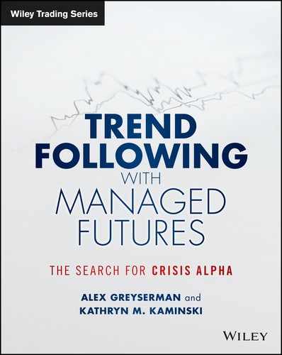
Because price risk is mean reverting over the long run, Sharpe ratios should also decrease over the long run if price risk sufficiently accounts for the total risk in a strategy. This means that when price risk accounts for risk, consistent with mean reversion, short-term Sharpe ratios should be lower than long-term. In specific terms, annual Sharpe ratios should be higher than monthly Sharpe ratios. Figure 9.6 plots the monthly, quarterly, and yearly Sharpe ratios for trend following (a strategy with high levels of price risk), using the DJCS Managed Futures Index as a proxy, and hedge fund strategies, using the DJCS Hedge Fund Index. From this graph, it is clear that especially in the short term, Sharpe ratios for hedge fund strategies are exposed to risks outside of price risk. Sharpe ratios are inflated in shorter horizons due to hidden risks. Sharpe ratios for trend following strategies are higher for longer horizons indicating that there are considerably less hidden risks in trend following.
FIGURE 9.6 Sharpe ratios for Dow Jones Credit Suisse Managed Futures Index and Dow Jones Credit Suisse Hedge Fund Index across different sampling frequencies.
Low Sharpe Ratios for Trend Following Are Prudent Performance Measures
Given the review of the four core risks in alternative investments, futures-based trend following strategies mostly contain price risk and even possibly leverage risk. This conclusion is consistent with intuition. As discussed in Chapter 2, futures strategies are highly liquid, efficient, low counterparty risk investments with minimal exposure to counterparty and liquidity risks. As a result, Sharpe ratios for trend following strategies prudently explain the amount of risk-adjusted return that is obtainable over time. In contrast, other alternative strategies that maintain other risks outside of price risk will have inflated Sharpe ratios that overstate performance in the short term. Because leverage risk depends on how a trend following system accelerates or decelerates positions, leverage risk is discussed in greater detail in the next few sections on dynamic leveraging.
■ Unraveling Hidden Risks of Dynamic Leveraging
Active derivatives-based trading strategies implicitly use leverage dynamically over time. Their use of leverage is often overlooked and misleading to investors. As a result, in this section, implicit leverage is explained. This helps to clarify how failing to properly evaluate for leverage may potentially glorify excessive risk taking. In simpler terms, it may be hard to distinguish the lucky big bettors from the calculated risk takers. This issue is important and unfortunately often overlooked by investors. A closer look at dynamic leveraging can help differentiate one trend following system from another.
For a futures manager, the simplest measure for the use of leverage is the margin to equity ratio. For example, many futures managers made exemplary returns in months like October 2008. A natural first question to ask: Is this due to luck or skill? If the return were due to luck, one would expect margin to equity ratios to be very high. This would mean that a manager took big bets (large notional positions) and they happened to pay off. For the month of October 2008, the opposite is actually true. Most trend followers were trading at margin to equity ratios well below their historical average. This means that their returns were skilled risk taking. In other words, if they had been taking more risks their returns would have been even larger than they already were. To put this into perspective, the October 2008 return for trend following was the highest from 2003 to 2013 while the margin-to-equity ratio was not even close to the highest. Given this example, it is clear that a closer look at how dynamic leveraging works and how it affects performance may help explain how to measure it, how to check for it, and how to evaluate when a manager is applying dynamic leveraging.
Defining Dynamic Leveraging
Dynamic leveraging is defined as a situation where the amount of leverage depends on the past profits and losses (PnL) of the portfolio. In simple terms, a dynamically leveraged portfolio, which increases (or decreases) its bet size when there are lots of past losers (or past winners), engages in a dynamic leverage strategy. Dynamic leveraging is similar to “doubling down” in poker. Dynamic leveraging is a convergent approach. Divergent strategies should cut their losses to manage risk. When divergent risk takers engage in dynamic leveraging, they are changing their approach to be convergent risk taking. Convergent strategies have a conviction regarding the structure of risks; when they are faced with a loss they will not cut the loss. In extreme cases, like dynamic leveraging, the approach will increase exposure to losing positions (a method of doubling down with position sizing).
dynamic leveraging a situation where the amount of leverage depends on the past profits and losses (PnL) in a portfolio.
Returning to the definition of dynamic leveraging, it is a situation where the amount of leverage depends on the past profits and losses (PnL) of the portfolio. For the example of options, the change in delta depends on the PnL of the option. Option selling is a simple type of dynamic leveraging. The delta (or the amount of shares of the underlying that are purchased using borrowed money) depends on the path of the underlying and the option’s underlying PnL. Take the example of an investor who sold a call option and the price goes up. The PnL for the option seller is a loss but the delta of the call option has increased. The option seller’s leverage also increases in tandem. For option sellers, leverage increases with losses and decreases with gains (or when the PnL is positive).4
The payoff characteristics and dynamic leverage use of option selling strategies can allow them to “get really lucky” in the short term, but the possibility that something can go devastatingly wrong in the longer term is nonnegligible. Put simply, dynamic leveraging, such as option selling, can be used to inflate performance in the short term. Dynamic leveraging is directly at odds with the divergent risk-taking approach.
Option Selling Strategies and Dynamic Leveraging
To compare the effects of dynamic leverage, a strategy such as option selling can be added to trend following. In this case, the performance for a representative pure trend following system, both with and without an option selling overlay, can be compared both long and short term.5 Position size is determined by the standard equal dollar risk approach from Chapter 3. The sample period for this analysis is from 2001 to 2013.
Option selling can be used as an overlay for trend following signals. When a trend following signal is positive (negative), the trend following system enters a short position in a put (call) option.6 The overlay forces the trend following strategy to systematically sell call and put options instead of taking linear futures positions. In the option-selling case, position size is determined by the option’s lambda and the volatility for each of the underlying markets. For simplicity in this example, option prices are calculated using the Black-Scholes formula. Figure 9.7 presents the performance of the crossover trend following system with and without the option selling overlay (both series are scaled to the same risk). During the 12-year sample period, the Sharpe ratio for the trend following system is 0.92 while the Sharpe ratio for the trend following system with the option selling overlay is 0.82.
FIGURE 9.7 Cumulative performance for a representative crossover trend following system with and without an option selling overlay. Both time series are scaled to the same monthly risk of 5 percent. The sample period is from 2001 to 2013.

Due to the specific payoff characteristic of option selling and its use of implicit dynamic leveraging, there exists a significant probability for an option selling strategy to achieve seemingly superior performance for shorter periods such as less than two years. Figure 9.8 plots the histograms for the two-year rolling Sharpe ratio of the trend following system with and without the option selling overlay. In this histogram, the option selling overlay allows the trend following system the possibility of achieving a higher Sharpe ratio in excess of 1.5 over a two-year period. Over longer periods of time, the Sharpe ratio of the system with option selling overlay becomes lower than the trend following system. In Figure 9.9, the probability of achieving a rolling Sharpe ratio higher than 1.5 is plotted versus the number of years in the rolling window for calculating the Sharpe ratio. For the one-year rolling Sharpe ratio, the option selling overlay system has a 38 percent chance to be above 1.5 compared with a probability of only 18 percent without the overlay. When the Sharpe ratio is examined over four years, neither of the approaches are able to achieve a Sharpe ratio above 1.5.
FIGURE 9.8 Histograms for two-year rolling Sharpe ratios for a trend following system with and without an option selling overlay. The sample period is from 2001 to 2013.

FIGURE 9.9 The probability of achieving a rolling Sharpe ratio higher than 1.5 versus the number of years for calculating the Sharpe ratio. The sample period is from 2001 to 2013.

Higher Sharpe ratios do not go unnoticed in higher order properties of returns. Higher short-term Sharpe ratios come at the cost of larger drawdowns and negative skewness. Without the overlay, the maximum drawdown is 26 percent; with the overlay, the maximum drawdown is 45 percent.7 Without the option selling overlay, the skewness is 0.51; with the overlay, the skewness becomes –0.34. Intuitively connecting to the convergent divergent discussion in Chapter 5, option selling is a convergent strategy; adding it to trend following adds hidden risks. Figure 9.10 presents histograms for another similar trend following system with and without an option selling overlay.
FIGURE 9.10 Histograms for monthly returns of the representative trend following system with (right panel) and without an option selling overlay (left panel) from 2001 to 2013.

Another less obvious consequence of dynamic leveraging is the reduction of crisis alpha. Using a VIX-based criteria8 to define crisis periods, Figure 9.11 plots the S&P 500 Index where the crisis periods are highlighted by the shaded bars. In this figure, 21 out of 129 months are defined as a crisis period. During the sample period from 2001 to 2013, Figure 9.12 presents the total return and crisis alpha for the trend following system with and without an option selling overlay. Based on the VIX definition of crisis, trend following returns 13 percent and delivers 5 percent crisis alpha. On the other hand, with the option-selling overlay the total return is 11.5 percent with a slightly negative crisis alpha at minus 0.5 percent. This simple comparison demonstrates how adding a convergent option-selling strategy overlay reduces crisis alpha for trend following. In summary, dynamic leveraging such as option selling gives access to higher short-term Sharpe ratios at the cost of deeper drawdowns, negative skewness, and loss of crisis alpha.
FIGURE 9.11 The S&P 500 Index with VIX-based crisis periods highlighted by the shaded bars.

FIGURE 9.12 Total return and crisis alpha for trend following with and without an option selling overlay from 2001 to 2013.

Martingale Betting and Dynamic Leveraging
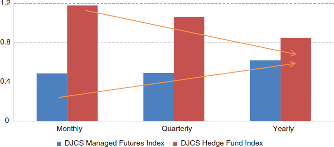
Martingale betting is another type of explicit dynamic leveraging. Martingale betting works in the following way: when faced with a loss, the long position is increased until the first day of positive PnL. Bets are increased when they are losing (another form of doubling down). If Martingale betting is applied to a trend following system, the number of double-downs days must be limited to remain tractable. In this case, the betting restarts when the number of consecutive days of loss reaches a predetermined number N or when the day’s PnL is positive. The number N puts a limit on the amount of doubling down that can occur. In a simple example, N is set to be a maximum of five days. This means that the futures manager can double-down (increase the exposure of a losing position) for at most five days. Figure 9.13 plots the cumulative performance of a representative trend following system with and without Martingale betting. Both time series are scaled to the same risk. At first glance, a Martingale betting scheme appears to improve the performance of trend following in this sample period. During the sample period of just over 10 years, the Sharpe ratio for the trend following system is 0.92 and the Omega ratio is 0.65.9 For the trend following system with a Martingale betting scheme, the Sharpe ratio is 1.09 and the Omega ratio is 1.20. This example creates a simple puzzle: How can a strategy with doubling down outperform a simple trend following system in terms of Sharpe ratio and Omega ratio? The answer is that these traditional measures ignore risks outside of price risk, not properly accounting for the use of dynamic leverage.
Martingale betting an explicit type of dynamic leveraging. Martingale betting works in the following way: a long position is increased until the first day of positive PnL. Bets are increased when they are losing (a form of doubling down).
FIGURE 9.13 The historical performance for a representative trend following system and a trend following system with dynamic leveraging (via limited Martingale betting) from 2001 to 2013.
In this section, dynamic leveraging is introduced with two simple approaches. First, option selling overlay strategies is a simple approach to add dynamic leveraging to trend following. This allows for access to higher Sharpe ratios in the short term at the expense of larger drawdowns, negative skewness, and the reduction of crisis alpha. Second, limited Martingale betting can be applied to trend following systems. In this case, doubling down increased the Sharpe ratio over the longer run, suggesting that aggressive dynamic leverage can be difficult to measure in high Sharpe ratios. Given that leverage risk may be hidden in traditional risk measures, the next logical step is to take a closer look at if or when dynamic leveraging occurs in trend following systems and how to measure it. Chapter 14 revisits dynamic leveraging and demonstrates how spectral analysis can help to filter out dynamic leveraging effects from Sharpe ratios. The next section discusses margin to equity and how it affects the portfolio volatility in trend following systems.
A Closer Look at Margin to Equity
The margin to equity ratio is a measure of the amount of traded capital that is being held as margin at any particular time. For example, if 25 percent of a fund’s capital was held in margin accounts for trading, the margin to equity ratio is 25 percent. A conservative trader may have a margin to equity ratio around 15 percent and an aggressive trader may be at 40 percent margin to equity. Because most contracts require roughly 5 to 10 percent in margin, each dollar in a margin account represents a leveraged exposure in the underlying contract. If a conservative futures trader has $100 and the margin requirement is 5 percent, he would put $5 into a margin account and take on one contract for $100. If an aggressive futures trader wanted to use more leverage, he could take on 5 contracts and put in $25 giving him an exposure of $500 notional, essentially levering up his investment. The margin to equity of the aggressive futures trader would be 25 percent and his gearing would be 4:1. All contracts vary in the amount of margin required. In aggregate, total margin to equity can be seen as a rough estimate of the amount of leverage being used. As futures traders change the size of their positions, add contracts, reduce contracts, and dynamically change their positions they dynamically change their leverage. The main question is: Do they use aggressive, so-called doubling down, dynamic leveraging such as in option selling strategies and Martingale betting? If there is excessive use of leverage, it may become a hidden risk in Sharpe ratios.
Margin to equity ratios in trend following systems are a rough measure of the amount of leverage that a system employs.10 If dynamic leveraging is applied, the amount of leverage will accelerate and decelerate more aggressively creating more volatility in margin to equity. As a result, the level of variability in the use of margin to equity can be examined to determine if dynamic leveraging is being applied. In more practical terms, the coefficient of variation for the daily margin to equity can be examined. The coefficient of variation for daily margin to equity measures the normalized dispersion of margin to equity. For the same representative trend following system from earlier in this chapter, the coefficient of variation for the daily margin to equity ratio is 0.3. In the case of limited Martingale betting, the coefficient of variation for the daily margin to equity is 0.5. Although this type of dynamic leverage does not show up in the Sharpe ratio, the use of dynamic leveraging such as in Martingale betting does create higher variability in margin to equity ratios (or a higher coefficient of variation).
coefficient of variation (for margin to equity) measure of the normalized dispersion of margin to equity.
The correlation between past levels of leverage (margin to equity) and the magnitude of future returns (both positive and negative) can also demonstrate the use of dynamic leveraging.11 If the correlation is high, past levels of high leverage resulted in the larger magnitude in returns (both positive and negative). This suggests that dynamic leveraging is being applied. Figure 9.14 presents scatter plots for daily positive and negative returns (absolute value) compared with lagged margin to equity for the representative trend following system. The correlation between lagged leverage and the magnitude of daily returns is relatively weak. More specifically, the correlation between the absolute value of daily negative returns and the lagged margin to equity is close to 0, and the correlation between the daily positive returns and the lagged margin to equity is even negative at –0.11. This suggests that trend following strategies do not engage in doubling down or the path dependent application of leverage such as option selling or Martingale betting. Higher returns for trend following most likely come from riding the price trend rather than the application of concentrated risks or dynamic leveraging.12 This point can be illustrated further with a specific example. In October 2008, the return for the representative trend following system was its highest at 17.5 percent and the average margin to equity ratio for the same month was 16 percent, which is lower than the average for all months in the whole sample period. As a counterexample, in April 2009, the return of the trend following system was –5.5 percent and the average margin to equity ratio for the same month was also 16 percent.13
FIGURE 9.14 Scatter plots for lagged margin to equity and the absolute value of negative daily returns (left panel) and positive daily returns (right panel) for the representative trend following system from 2001 to 2013.

For comparison purposes, dynamic leveraging can be added to a trend following system. In this case, the correlation between the absolute value of daily negative returns and the lagged margin to equity ratio goes from close to zero to 0.37, and the correlation between positive returns and the lagged margin to equity ratio goes from –0.11 to 0.46. Figure 9.15 shows scatter plots for the negative daily returns (absolute value) and positive returns with lagged margin to equity ratios. For the case of limited Martingale betting, the magnitude of returns is often derived from higher leverage.
FIGURE 9.15 Scatter plots between the lagged margin to equity and the absolute value of negative daily returns (left panel) and positive daily returns (right panel) of the trend following system with limited Martingale betting from June 2001 to February 2012.

In the case of dynamic leveraging, margin to equity ratios experience spikes in their volatility. This indicates that there may be hidden leverage risk. Figure 9.16 shows a comparison of the daily 22-day rolling volatility for the representative trend following system with and without a Martingale betting scheme. When both systems’ monthly risks are scaled to 5 percent, their volatility behaves strikingly different across time. For the Martingale betting scheme, on a daily basis, volatility exhibits a cyclical pattern. The Sharpe ratio calculated by daily returns for Martingale betting should be expected to be quite different from the typical Sharpe ratio based on monthly returns. The aggregation of daily returns conceals the highly volatile daily path in PnL.14 When daily data is used, the Sharpe ratio is reduced by roughly 20 percent. For the representative trend following system, the Sharpe ratios based on both daily and monthly returns are similar.
FIGURE 9.16 22-day rolling volatility for the representative trend following system and with Martingale betting.

■ Summary
In this chapter, the core risks in alternative investment strategies were reviewed. These risks include price risk, credit risk, liquidity risk, and leverage risk. By comparing trend following with other alternative investment strategies, price risk and leverage risk were shown to be two main risks to discuss for trend following. By reviewing Sharpe ratios in contrast with key risks in alternatives, most risks in alternative investment strategies are hidden in Sharpe ratios. For the case of trend following that takes on only price risk, Sharpe ratios are prudent measures of risk taking with one caveat that needs to be examined further, leverage. If a strategy applies dynamic leverage, similar to doubling down in option selling or Martingale betting schemes, there may be leverage risk hidden in Sharpe ratios as well. A closer look at margin to equity ratios over time demonstrates that trend following strategies do not use dynamic leverage.
■ Further Readings and References
Brunnermeier, M., and L. Pedersen. “Market Liquidity and Funding Liquidity.” Review of Financial Studies 22, no. 6 (2009): 2201–2238.
Foster, D., and H. Young. “The Hedge Fund Game: Incentives, Excess Returns, and Piggy-Backing.” Working paper, 2007.
Getmanksy, M., A. Lo, and I. Makarov. “An Econometric Model of Serial Correlation and Illiquidity in Hedge Fund Returns.” Journal of Financial Economics 74 (2004): 529–609.
Goetzman, W., J. Ingersoll, M. Spiegel, and I. Welch. “Sharpening Sharpe Ratios.” NBER Working Paper No. 9116, 2002.
Greyserman, A. “Dynamic Leveraging as a Factor of Performance Attribution.” ISAM white paper, 2011.
Kaminski, K., and A. Mende. “Crisis Alpha and Risk in Alternative Investment Strategies.” CME Group white paper, 2011.
Keating, C., and W. Shadwick. “A Universal Performance Measure.” London: The Finance Development Centre, 2002.
Khandani, A., and A. Lo. “Illiquidity Premia in Asset Returns: An Empirical Analysis of Hedge Funds, Mutual Funds, and U.S. Equity Portfolios.” Working paper, 2010.
Lo, A. W. “Risk Management for Hedge Funds: Introduction and Overview.” Financial Analysts Journal 57, no. 6 (November/December 2001).
Lo, A. W. “The Statistics of Sharpe Ratios.” Financial Analysts Journal 58, no. 4 (July/August 2002).
Sharpe, W. F. “The Sharpe Ratio.” Journal of Portfolio Management 21, no. 1 (Fall 1994): 49–58.
Smith, S. W. “The Scientist and Engineer’s Guide to Digital Signal Processing.” California Technical Pub., 1997.
Vayanos, D. “Flight to Quality, Flight to Liquidity, and the Pricing of Risk.” NBER Working Paper, 2004.
1 One caveat—dynamic investment strategies are typically a mix of convergent and divergent risk taking. Pure trend following is both a directional strategy and a divergent strategy. It avoids hidden risks common in convergent strategies. As a counterexample, a long volatility strategy that buys out-of-the-money OTC options applies divergent risk taking by limiting losses to the purchase of the option and riding the option payout in extreme events. Despite this, these long volatility strategies maintain and must manage some credit/via counterparty risk and liquidity risk.
2 The discussion in this section is directly related to Kaminski and Mende (2011). Negative crisis alpha indicates losses during crisis as opposed to gains. Source: RPM and the CME Group.
3 Khandani and Lo (2010) discuss the existence of an illiquidity premium. The use of autocorrelation as a proxy for liquidity risk is also discussed in Getmanksy, Lo, and Makarov (2004) in regard to systemic risk in hedge funds.
4 Option selling is a convergent risk-taking strategy. The strategy takes small profits and has unbounded exposure on the downside similar to doubling down betting schemes. This type of convergent risk taking clearly adds hidden risks to Sharpe ratios.
5 A moving average crossover representative trend following system is used for this analysis. This system trades across a diversified universe of markets: commodity, fixed income, stock index, and FX sectors. In these experiments, shorter lookback window sizes range from 10 to 30 days and longer lookback window sizes range between 60 and 250 days.
6 For simplicity, the trend following system enters an at-the-money option. Despite this assumption, the conclusions of this analysis are general and do not depend on the specific choices of parameters.
7 Both are scaled to the same monthly risk of 5 percent.
8 A month is defined to be a crisis period when the percentage change in the VIX is greater than 20 percent. This approach is consistent with several academic papers on this topic: see Vayanos (2004) and Brunnermeier and Pedersen (2009).
9 A threshold of 2 percent is used for the Omega ratio. The Omega ratio is discussed in the appendix of Chapter 7.
10 For the calculations in this section, in order to estimate margin a multiplier of 10 percent is applied to the gross exposure of markets in commodities, stock indices, and FX. A multiplier of 1 percent is applied to the gross exposure of fixed income to estimate margin.
11 The margin to equity ratio is lagged by one day. This is because the return on day T depends on the positions at day T-1.
12 In Chapter 8, this concept was discussed for the case of drawdowns. Trend following drawdowns are caused by lots of small losses as opposed to large concentrated bets.
13 This effect can be called asymmetric leverage.
14 This is especially true if Martingale betting is applied earlier in the month.