CHAPTER 16
Diversifying the Diversifier
Diversification is the act of introducing variety into an investment portfolio. Diversification is often touted as the only method to achieve some protection during periods of distress. For an investment manager, diversification can be either intrastrategy or interstrategy. For example, Chapter 15 discussed how fund size can impact intrastrategy diversification by limiting access to smaller, less liquid markets as well as examining statistics that affect interstrategy diversification benefits at the total portfolio level. This chapter focuses on diversification at an interstrategy or total portfolio level and discusses the prospect of moving from pure trend following into a more multistrategy approach. The empirical analysis in this chapter demonstrates that, on a stand-alone basis, a multistrategy approach may be beneficial to a trend following manager. Despite this, from an outside perspective, diversifying away from trend following may decrease some of the desirable properties in a larger portfolio context. More explicitly, the move from pure trend following to multistrategy results in reducing both the positive skewness and the potential for delivering crisis alpha. To demonstrate this more explicitly, portfolio benefits of a pure trend following program versus a multistrategy approach are compared empirically from the perspective of an institutional investor. From the perspective of the manager, a multistrategy approach may be desirable, but from the perspective of an external investor it may be less desirable. Given that relative value strategies and many other hedge fund strategies tend to be convergent strategies, this chapter also returns to issues related to hidden risk in the use of nondirectional convergent strategies.
intrastrategy or interstrategy intrastrategy are differences internal to a strategy and interstrategy are differences between external strategies.
intrastrategy or interstrategy intrastrategy are differences internal to a strategy and interstrategy are differences between external strategies.
■ From Pure Trend Following to Multistrategy
The move from pure trend to multistrategy has been increasingly popular in the CTA space. It is conceivable that adding nontrend strategies may be a simple way to increase Sharpe ratios over time. As discussed in Chapter 9, there are often hidden risks in high Sharpe ratios. In addition to the quantitative benefits, there are other concerns for an investor regarding the move to multistrategy. Most importantly, the shift from pure divergent strategies like trend following into convergent strategies makes a trend following strategy more similar to the underlying portfolios of investors. Other issues also include the constant concern of style drift, clarity of investment process, and transparency.
By taking a closer look at the statistical properties of a multistrategy approach in contrast with pure trend following, the pros and cons of this approach can be examined more explicitly. This section takes a first look at the impact of a multistrategy approach on Sharpe ratios, portfolio skewness, and crisis alpha. This analysis provides the background for an empirical analysis of portfolio performance from the perspective of an institutional investor in the next section.
Sharpe Ratios
Chapter 9 discussed the myths and mystique of the Sharpe ratio as a performance measure. Nondirectional strategies may introduce hidden risks in investment strategies. More specifically, this means that adding nondirectional strategies may increase Sharpe ratios without exposing the potential for hidden risks. To demonstrate this, a simple multistrategy CTA can be modeled by combining the return series of a representative trend following system with the HFRI Fund of Funds (FoF) index. The return of the HFRI Fund of Funds index is used as a simple proxy for a pool of diversified nontrend following strategies. The empirical results are based on a diversified universe of markets inclusive of equity indices, bonds, rates, FXs, and commodities.
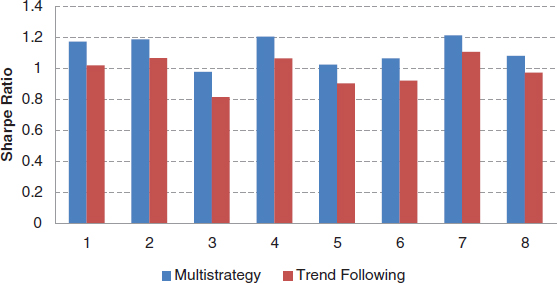
In this simulation at the end of each month, 80 percent risk is allocated to trend following and 20 percent risk is allocated to the HFRI FoF index. As shown in Figure 16.1, the multistrategy portfolio is able to improve the standalone performance for all trend following strategies. At first glance, this may seem appealing as the move from pure trend following to multistrategy increases Sharpe ratio for a CTA manager on a standalone basis. To understand the implications for diversification, other desirable statistical properties such as negative skewness and crisis alpha should also be examined.
FIGURE 16.1 Sharpe ratios for each trend following system with a 20 percent risk allocation to the HFRI FoF index (multistrategy).
Data source: Bloomberg.
Negative Skewness
One of the desirable return characteristics of a divergent trading strategy like trend following is positive skewness. Most hedge fund strategies are convergent trading strategies and they exhibit negative skewness. Figure 16.2 plots a comparison of skewness in monthly returns between a pure trend follower (pure TF System) and a variety of other strategies. From this figure, it is evident that pure trend following is one of the few strategies with very positive skewness in returns. Other hedge fund strategies tend to be negatively skewed.
FIGURE 16.2 Monthly return skewness for pure trend following (Pure TF System) and a variety of other strategies.
Data source: Bloomberg.

Skewness measures the degree of asymmetry in a distribution. A negatively skewed distribution has a long tail on the left side of the mean, while positive skewness indicates a long tail on the right side. To put the skewness values into perspective, Figure 16.3 illustrates the probabilities of a monthly return series generating a return below x percent, where x ranges from –5 to –9 percent, at various skewness levels.1 Note that, though all the return series have the same Sharpe ratio, the probability of achieving an outsized negative return diverges significantly across different skewness levels, for example, the probability of achieving a return below –5 percent at skewness –1.0 is more than twice that of a distribution with skewness of 1.0.
FIGURE 16.3 The probability that a monthly return series achieving a return below x percent for various levels of skewness: x ranges from –5 to –9 percent.

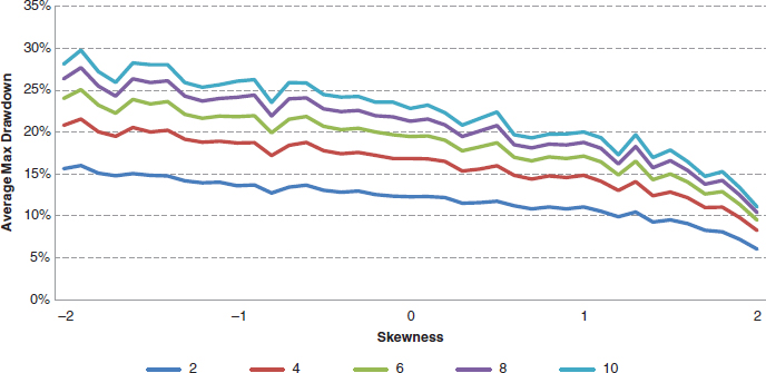
Skewness in returns also has a direct impact on the expected value of maximum drawdown. Negatively skewed returns have higher maximum drawdowns and vice versa. Using a simple Monte Carlo simulation, Figure 16.4 displays the expected maximum drawdown in n years, 2 ≤ n ≤ 10, at each skewness level for the various return series depicted with the same Sharpe ratio. A positively skewed return distribution is expected to have a much lower maximum drawdown than a negatively skewed distribution.
FIGURE 16.4 Average maximum drawdown in a period of n years, for 2 ≤ n ≤ 10, for a range of return skewness levels. Each simulated return series has the same Sharpe ratio.
The act of adding convergent, negatively skewed, trading strategies to a trend following strategy will decrease the positive skewness. This can potentially undermine the benefits of trend following such as decreasing maximum drawdowns from a total portfolio perspective.
Crisis Alpha
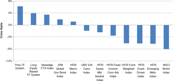
Crisis alpha measures a strategy’s performance during market stress. It is one of the most important portfolio benefits of trend following. Figure 16.5 shows the crisis alpha of pure trend following and several other hedge fund strategies and indices during equity market crises.2 Although most other hedge fund strategies and indices provide negative crisis alpha, the pure trend following system provides a monthly crisis alpha of 6 percent. Given the performance of most traditional portfolios during market crisis, crisis alpha provides substantial diversification benefits for an institutional investor. The impact of trend following strategies is examined from a total portfolio perspective in the following sections.
FIGURE 16.5 Crisis alpha for pure trend following (Pure TF System) and several other strategies and indices.
Data source: Bloomberg.
■ Portfolio Analysis of the Move to Multistrategy
From the perspective of a CTA manager, the move from pure trend following to multistrategy may increase Sharpe ratios, especially in the short run. On the other hand, with the traditional 60/40 or fund-of-funds, institutional investors already hold a significant allocation to nontrend following strategies. From the perspective of the institutional investor, the move from pure to multistrategy may degrade some of the portfolio benefits of investing in CTAs in general. To demonstrate this, a simple multistrategy CTA can be modeled by combining the return series of a representative trend following system with the HFRI Fund of Funds (FoF) index. The return of the HFRI Fund of Funds index is used as a simple proxy for a pool of diversified nontrend following strategies. This proxy is only one proxy and results for other nontrend strategies may vary. The empirical results are based on the 20-year period between 1993 and 2013, using a diversified universe of markets inclusive of equity indexes, bonds, interest rates, FXs, and commodities. In the following two sections, the move to multistrategy is examined first from the perspective of the 60/40 investor and second from the perspective of the fund of funds investor. The performance statistics are compared both across different trend following substrategies to provide perspective on the dispersion in portfolio benefits. Lastly, robustness of the results is discussed in the absence of bonds and across multiple time periods.
The 60/40 Investor
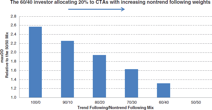
The 60/40 investor is represented by combining a 60 percent allocation to the MSCI World Index and 40 percent allocation to the JP Morgan Global Bond Index. Figure 16.6 depicts the five-year rolling Sharpe ratio of the 60/40 portfolio combined with a 20 percent allocation to either a pure trend following system or a multistrategy CTA.3 From 1998 to 2013, the portfolio with 20 percent pure trend following achieved a higher Sharpe ratio. In particular, when the traditional 60/40 portfolio is in a significant drawdown, the pure trend following strategy benefits the investor more significantly than the multistrategy CTA. To put this into further perspective, Figure 16.7 plots the deteriorating drawdown profile as a CTA allocates more risk to nontrend following strategies. For example, when a multistrategy CTA is compared with a 50/50 allocation to nontrend following strategies and a pure trend following program, pure trend following has a 2.5 times larger impact on drawdown reduction. Both improved long-term Sharpe ratios and better drawdown reduction demonstrate how from a global portfolio perspective a multistrategy approach may be less desirable.
FIGURE 16.6 Five-year rolling Sharpe ratio for a representative trend following system and a multistrategy CTA plotted together with the cumulative performance of a traditional 60/40 strategy. The sample period is from 1998 to 2013.
Data source: Bloomberg.

FIGURE 16.7 Maximum drawdown relative to a 50/50 allocation to trend following mix of trend and nontrend strategies as a function of the percentage invested in pure trend following to nontrend strategies. The vertical axis is the ratio between the maximum drawdown reduction of the various allocations to nontrend following strategies and that of the 50/50 allocation. The sample period is from 1998 to 2013.
The Fund-of-Funds Investor
As with the traditional 60/40 investor, a fund-of-funds investor observes the same disparity of portfolio benefits between a pure trend following strategy and a multistrategy CTA. Using the HFRI FoF index as a proxy for the portfolio of a fund-of-funds investor, Figure 16.8 displays the five-year rolling Sharpe ratio of a portfolio combining a traditional fund-of-funds investment with an allocation to a CTA in an 80/20 ratio. CTAs in the analysis are a pure trend follower and a multistrategy CTA with 50 percent of risk taken in nontrend following methodologies.4 Similar to the 60/40 investor, over a 20-year period, the fund-of-funds portfolio combined with a 20 percent allocation to pure trend following, achieved a higher Sharpe ratio. In cases where the HFRI FoF index is in a significant drawdown, pure trend following strategies benefit the investor more significantly than the multistrategy CTA. Consistent with the drawdown profiles for the 60/40 portfolio, Figure 16.9 presents a similar pattern for the fund of fund portfolio for maximum drawdowns as a CTA allocates more risk to nontrend following strategies. For example, when a multistrategy CTA is compared with a 50/50 allocation to nontrend following strategies with pure trend following, the impact on drawdown reduction is 3.1 times larger for the pure trend following approach.
FIGURE 16.8 Five-year rolling Sharpe ratios for the fund of funds portfolio combined with 20 percent of the representative trend following system and a multistrategy CTA, respectively, plotted with the cumulative performance of the HFRI FoF Index.
Data source: Bloomberg.

FIGURE 16.9 Maximum drawdown for a fund of funds (FoF) investor with an increasing allocation to nontrend strategies. The vertical axis is the ratio between the maximum drawdown reduction of the various allocations to nontrend following strategies and that of the 50/50 allocation. The sample period is from 1993 to 2013.

The Disparity of Portfolio Benefits and System Design
The previous section demonstrates and documents how the move from pure trend following to multistrategy may improve Sharpe ratios on a standalone basis while potentially deteriorating the portfolio benefits of pure trend following. To document the robustness of these effects, portfolio benefits are compared across eight trend following systems, described in Table 16.1. Portfolio benefits are examined in terms of Sharpe ratio improvement, maximum drawdown reduction, and change in beta.5 Figure 16.10 plots the Sharpe ratio improvement after the 60/40 portfolio is combined with 20 percent overlay of either a trend following portfolio or a multistrategy CTA portfolio. Both approaches can improve the Sharpe ratio consistently, but the benefit of a multistrategy CTA is consistently lower than the corresponding trend following systems. From Figure 16.11 depicting the reduction of maximum drawdown, the same conclusion can be made. Based on maximum drawdowns, a pure trend following portfolio delivers more significant benefits to a 60/40 portfolio. In Figure 16.12, the pattern for the change in beta is somewhat mixed, but it is still relatively consistent that a multistrategy CTA fund is less effective at reducing the beta of the portfolio.
TABLE 16.1 Eight trend following systems along three dimensions: equity bias, capital allocation, and holding horizon. Here, “No Long Horizon” indicates a median horizon.
Equity Long Bias |
Market Capacity Weighted |
Long Horizon |
|
| 1 | No |
No |
No |
| 2 | Yes |
No |
No |
| 3 | No |
Yes |
No |
| 4 | No |
No |
Yes |
| 5 | Yes |
Yes |
No |
| 6 | No |
Yes |
Yes |
| 7 | Yes |
No |
Yes |
| 8 | Yes |
Yes |
Yes |
FIGURE 16.10 Sharpe ratio improvement after the 60/40 portfolio is combined with 20 percent overlay of either a trend following portfolio (Systems 1 to 8) or a multistrategy CTA (with Systems 1 to 8).
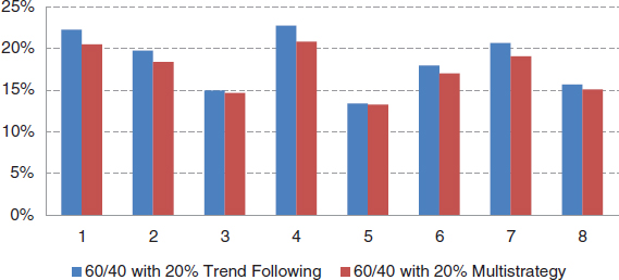
FIGURE 16.11 Maximum drawdown reduction after the 60/40 portfolio is combined with 20 percent overlay of either a trend following portfolio (Systems 1 to 8) or a multistrategy CTA (with Systems 1 to 8).
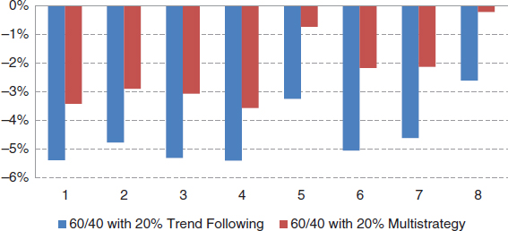
FIGURE 16.12 Change in beta (using the MSCI World Index) after the 60/40 portfolio is combined with 20 percent overlay of either a trend following portfolio (Systems 1 to 8) or a multistrategy CTA (with Systems 1 to 8).

After comparing trend following with a multistrategy CTA and an examination of the traditional 60/40 investor, now the portfolio benefits of each trend following system can be examined in more detail for the fund of funds (FoF) investor. Figure 16.13, Figure 16.14, and Figure 16.15 show Sharpe ratio improvement, reduction of maximum drawdown, and beta change after the 60/40 portfolio and the HFRI FoF index are combined with the 20 percent overlay of the average returns of each subspace. Pure trend following (System 1 and System 4, with the latter being a slower system) consistently provides the largest portfolio benefits in terms of Sharpe ratio improvement, maximum drawdown reduction, and beta reduction. This conclusion stands for both the traditional 60/40 investors and the fund of funds (FoF) investors.
FIGURE 16.13 Sharpe ratio improvement for the 60/40 portfolio and HFRI FoF Index when combined with a 20 percent overlay from each of the eight trend following systems.

FIGURE 16.14 Reduction in maximum drawdown for the 60/40 portfolio and HFRI FoF Index when combined with a 20 percent overlay of each of the eight trend following systems.
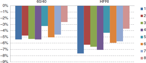
FIGURE 16.15 Change in beta (using the MSCI World Index) for the 60/40 portfolio and HFRI FoF Index when combined with a 20 percent overlay from each of the eight trend following systems.

The Robustness of Portfolio Benefits
The empirical results in the previous sections are derived from a diversified universe of markets consisting of equity indexes, bonds, interest rates, FXs, and commodities. The past 20 years represent a period of prolonged falling interest rates. This long-term trend has played a major role in trend following performance (as all trends should). Despite this, removing bonds from the portfolio may provide some indication how much of the results may depend on bonds or on even the most recent extreme low interest rate environment. To gauge the robustness of portfolio benefits, this section provides two alternative views: the absence of bonds for the entire period and a closer look at the recent 10 years where interest rates have decreased to extremely low levels. For the sake of brevity, the discussion is focused on the Sharpe ratio improvement.
The Absence of Bonds Trend following has clearly benefited by capturing the strong trends created by an extended falling interest rate environment over the past several decades. Currently, interest rates are near historically low levels; investors are naturally concerned about the potential impact of a rising rate environment on trend following. In both the multicentennial analysis in Chapter 1 and the discussion of interest rate environments in Chapter 6 and Chapter 10, rising interest rate environments are not necessarily detrimental to trend following performance. Despite this, there have been substantial trends in fixed income during the past 20 years. To isolate the impact of portfolio benefits in absence of this rather large trend, it is interesting to examine the portfolio benefits of trend following in the absence of bonds. Figure 16.16 shows the comparison between the Sharpe ratio improvement (upper panel) and maximum drawdown reduction (lower panel) for both the 60/40 portfolio and HFRI FoF index when the trend following portfolio acts inclusive and exclusive of bond markets. Although the exclusion of bond markets does reduce the magnitude of Sharpe ratio improvement, with comparatively more impact on the fund-of-funds investor, the Sharpe ratio still remains positive. Moreover, it appears that the maximum drawdown reduction for both investor types is largely indifferent to the removal of bond markets in a trend following program.
FIGURE 16.16 The impact on the Sharpe ratio improvement and maximum drawdown reduction both with and in the absence of fixed income using a 20 percent allocation to trend following for both the 60/40 portfolio and the HFRI FoF Index.

To examine the impact of bonds at a more granular level, different types of trend following systems can be examined. Figure 16.17 shows the comparison between the Sharpe ratio improvement for both the 60/40 portfolio and HFRI FoF Index when the trend following portfolio includes or excludes bond markets. For trend following System 4 and System 7, the absence of bond markets does not appear to reduce the Sharpe ratio improvement substantially. However, for the trend following systems with the market capacity based allocation, for example, trend following Systems 3 and 5, the negative impact for the absence of bonds is more significant. As discussed in Chapter 15, the fixed-income futures markets are the largest and most liquid.
FIGURE 16.17 The impact of removing fixed income from trend following portfolios in terms of Sharpe ratio improvement for both the 60/40 portfolio and the HFRI FoF Index. Each index has a 20 percent allocation to trend following with or without fixed income.

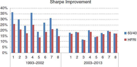
Time Periods To evaluate the robustness of portfolio benefits through time, the 20-year sample period can be split into two separate 10-year periods. Figure 16.18 compares the Sharpe ratio improvement (upper panel) and maximum drawdown reduction (lower panel) for the two separate decades for both the 60/40 portfolio and the HFRI FoF Index. Interestingly, the Sharpe ratio improvement for the 60/40 portfolio is noticeably lower in the more recent 10 years, but the benefit to the HFRI FoF Index has been relatively robust throughout. The impact on maximum drawdown has been more stable in both time periods.
FIGURE 16.18 A comparison of Sharpe ratio improvement and maximum drawdown reduction using a 20 percent of allocation to trend following over time periods (1993–2002 and 2003–2013) for both the 60/40 portfolio and the HFRI FoF Index.

It appears that portfolio benefits for the 60/40 portfolio are noticeably lower in the more recent 10 years, but the benefit for the HFRI FoF Index is relatively robust. Overall, significant portfolio benefits can be observed in the more recent past for both types of institutional portfolios. Moreover, in both decades, pure trend following strategies (System 1 and System 4) consistently provide larger benefits to an institutional investor.
In this section, it was observed that despite increasing Sharpe ratios on a standalone basis, a multistrategy CTA with an allocation to nontrend following strategies may provide reduced portfolio benefits for institutional portfolios. To demonstrate the robustness of this conclusion, the disparity of portfolio benefits between distinctive trend following programs was also discussed. Empirical results show that pure trend following, characterized by system symmetry and equal dollar risk allocation, achieves the largest portfolio benefits for both traditional 60/40 traditional investors and fund of funds investors. This analysis provides some important insights into the move from pure trend following to multistrategy approaches in the managed futures space. From the perspective of an investor, they must decide what their objective is. If they are looking for a one-stop shop with a higher Sharpe ratio, a multistrategy approach may make sense. If, on the other hand, an investor already holds a diversified nontrend portfolio, they may invest in trend following for diversification. In this case, the move from pure trend following to multistrategy may be more in the best interest of a CTA manager than an institutional investor seeking diversification.
FIGURE 16.19 The impact of different time periods (1993–2002 and 2003–2013) in terms of Sharpe ratio improvement from adding trend following for both the 60/40 portfolio and the HFRI FoF Index. Each index has a 20 percent allocation to trend following.
■ Hidden Risk of Leveraging Low-Volatility Strategies
Although there are many ways to diversify a trend following program interstrategy, a common method is to add purely convergent risk-taking strategies such as relative value.6 These strategies often have high Sharpe ratios especially over shorter periods of time. To achieve adequate returns, they often also require substantial use of leverage. The use of leverage magnifies the impact of tail risks in convergent risk-taking strategies. This section discusses the hidden risks (or tail risks) in leveraging low-volatility relative value strategies.7 For this discussion, a generic long/short relative value strategy is considered. This long/short strategy involves two highly correlated portfolios, one long and one short, both with the same dollar risk (σ). If the long and short legs of the relative value strategy have correlation (ρ), the volatility of the relative value strategy (σRV) can be expressed by the following expression:
![]()
when ρ > 0.5, the volatility of the relative value strategy (σRV) is lower than (σ). Due to the typically strong correlation between the long and short portfolios, standard portfolio theory suggests that the long/short relative value strategy’s volatility becomes quite low as correlations increase. For example, if correlation is 0.9 and volatility is 20 percent, the relative value strategy has a net volatility of 8.94 percent (much lower than 20 percent). In a portfolio consisting of strategies with heterogeneous risk profiles, significant leverage is often necessary to maintain equal risk for low-volatility strategies of this type. Using even simple risk budgeting techniques, required leverage can be substantial.
Consider first a hypothetical portfolio consisting of a long/short relative value strategy and two other managed futures strategies. In a simple case, both the long and short leg of the relative value strategy have risk of (σ) and both managed futures startegies have risk of (σ). To achieve equal dollar risk allocation between the three portfolios, a leverage factor of n (where n > 1) would need to be applied to the relative value strategy. In this specific case, the required leverage would be as follows:

For the case when the correlation is 0.9, the required leverage factor is 2.24. When the correlation is 0.98, the required leverage factor is 5.8 In the case with three strategies, the relative value strategy has a risk exposure of ⅓ or 33 percent. Instead of net risk exposure, gross risk exposure can also be considered. The gross leveraged risk level of the relative value strategy is 2nσ. In the case when both of the two other strategies have the same risk (σ), the net and gross risk exposures for the relative value strategy can be characterized by the following:

For example, when the correlation is 0.9, n is 2.24. The net exposure for the relative value strategy is 33 percent but the gross exposure is 69 percent. This example shows how the gross risk exposure for a low-volatility relative value strategy can be much higher than the net exposure when using an equal risk approach. High gross risk exposure can lead to an increased chance for potentially disastrous left tail events.
When the long and short portfolios experience opposite and potentially detrimental moves simultaneously, the ensuing negative strategy return will be exacerbated by the leverage factor. It is important to examine how likely it is that the long-short portfolio experiences an adverse move. Under the assumption of a multivariate normal distribution in the long and short portfolios’ returns, at various levels of leverage and correlation between the long and short portfolios, Figure 16.20 displays the probability of the relative value strategy having a return of −2σ or lower, relative to the probability (2.3 percent) of a normal distribution having a return of −2σ or lower. The ratio between the probabilities of returning −2σ or lower in both the relative value strategy and the normal distribution is called a tail risk multiplier. For example, when a relative value strategy has a correlation between the long and short portfolios of 0.75 and a leverage factor of 4, the resulting tail risk multiplier is 10. The tail risk multiplier indicates that the probability of the relative value strategy returning −2σ or lower is 10 times more likely than the normal distribution.
tail risk multiplier the ratio between the probability of returning a value two standard deviations or lower to the probability of the normal distribution returning a value two standard deviations or lower. For a particular returns series, if the probability is 10 times the normal distribution, the tail risk multiplier is 10.
FIGURE 16.20 The probability of the relative value strategy returning −2σ or lower, as a ratio relative to the probability (2.3 percent) of a normal distribution returning −2σ or lower, at various leverage levels and correlations between the long and short portfolios.

Further complications can arise when the correlation between the long and short portfolios changes significantly. When this correlation decreases, the volatility of the relative value strategy (σRV) will increase accordingly. Figure 16.21 shows the volatility increase of the strategy when the correlation is decreased by 0.1 for various original correlation values with leverage varying from 1x to 5x.9 When the original correlation is higher, the marginal increase in volatility due to the correlation decrease is larger. In addition, when leverage is higher, the marginal increase in volatility is also higher.
FIGURE 16.21 The increase in risk when the correlation decreases by 0.1 for different leverage levels (n) as a function of the original correlation.

As correlations change, this has several implications for the risk of a combined portfolio. First, the original equal risk allocation between the portfolios is no longer equal. As such, the relative value strategy’s risk allocation can be substantially higher than the original budget. Secondly, as shown in Figure 16.20, when the correlation between the long and short portfolios decreases, the probability of “going wrong,” left tail events, or large adverse moves becomes higher.
High gross risk exposure can lead to potentially disastrous consequences. In the worst case, where both the long and short portfolios have a 0.5 standard deviation move in an unexpected, opposite direction, these moves of the long-short portfolio will be amplified at the total portfolio level due to leverage. For an unexpected, opposite m-standard deviation move for both the long and short portfolios, the corresponding move at the whole portfolio level can be written as:
![]()
where (ΔPtot) is the change in the total portfolio, (n) is the leverage factor and (k) is the multiplier for the whole portfolio’s dollar risk relative to the individual portfolio’s dollar risk. Depending on the correlations between the strategies, a 0.5 standard deviation move can cause roughly an n-standard deviation move for the whole portfolio.
When the long portfolio experiences a substantial negative move and the short portfolio experiences a substantial positive move simultaneously, the leverage factor will exacerbate the effects. It is important to consider how likely it is that a move will go in the wrong direction for a relative value strategy. Using the assumption of a multivariate normal distribution for the long and short portfolios’ returns, the joint probability of negative 0.5-standard deviation move for the long portfolio and a positive 0.5-standard deviation move for the short portfolio simultaneously can be calculated as a function of the correlation between the long and short portfolios.
Figure 16.22 demonstrates that, even when correlation is high between the long and short portfolios within the relative value strategy, the probability for a long-short portfolio to go wrong is not negligible. Based on these probabilities at a leverage factor of 3 and correlation value of 0.7 between the long and short portfolios, the relative value strategy has a 1.5 percent chance of making a negative 3-standard deviation move. To put this move into perspective, for a normal distribution the chance of a negative 3-standard deviation move is only 0.1 percent.
FIGURE 16.22 The joint probability of a negative 0.5-standard deviation move for the long portfolio and a positive 0.5-standard deviation move for the short portfolio as a function of the correlation between the long and short portfolios.
The Impact of Variant Correlation
In reality, correlations are not constant across time. When correlation decreases between the long and short portfolios, the risk for the relative value strategy increases. Figure 16.23 shows the risk increase when the correlation decreases by 0.1 for different leverage levels as a function of the original correlation.10 When correlation is higher, the marginal increase in risk due to the correlation change is higher. When leverage is higher, the marginal increase in risk is also higher.
FIGURE 16.23 The increase in risk as correlation decreases for different leverage levels as a function of the original correlation.

Correlation changes have several implications on risk. First, as correlations change, the original equal risk allocation between the three portfolios does not remain equal. The relative value strategy’s risk allocation can be substantially higher than what it was set at the time of allocation. Second, as shown in Figure 16.23, the probability of going wrong becomes higher as the correlation between the long and short portfolios decreases.
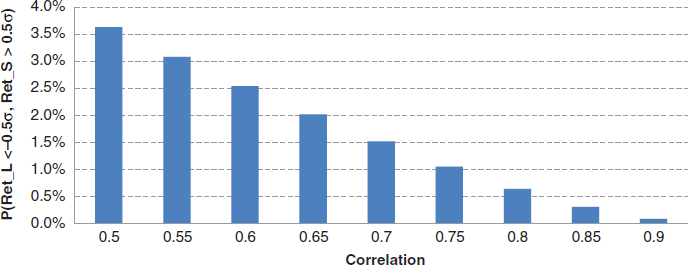
The probability that the relative value strategy experiences a two-standard deviation adverse move for the entire portfolio can also be estimated.11 Figure 16.24 displays the increased probability for the whole portfolio having a negative two-standard deviation move due to the correlation decrease between the long and short portfolios of the relative value strategy.12 A change in correlation from 0.9 to 0.7 would increase the probability by 10 percent for the relative value strategy to experience a two-standard deviation or larger adverse move for the entire portfolio.
FIGURE 16.24 The increase in probability for the entire portfolio to have an adverse move of two-standard deviations or more as a function of the correlation decrease between the long and short portfolios in the relative value strategy.

■ Summary
Most investors cite diversification benefits as one of the key reasons for investing in trend following. Despite the appeal of a pure trend following approach, there is an increased trend from pure trend following to multistrategy. This chapter presents both a discussion of this move and the impact of a multistrategy approach on the diversification benefits of trend following. Multistrategy CTAs boast higher Sharpe ratios on a standalone basis but the move to multistrategy comes at the cost of less desirable correlation with traditional portfolios, less drawdown reduction, reduced crisis alpha, and less positive skewness. For both a 60/40 and a fund of funds (FoF) investor, the move to multistrategy reduces the diversification benefits of trend following across a wide range of trend following approaches. The results of this analysis are robust for shorter horizons and in the absence of fixed income. Because many multistrategy CTAs may consider adding convergent relative value strategies or low-volatility strategies as a general class, the final section of this chapter returned to the discussion of hidden risks for leveraging low-volatility strategies. The necessity to leverage for equal risk portfolios was used to demonstrate how adverse moves in relative value strategies are magnified by leverage at the portfolio level. This discussion provides a more detailed view into the hidden risks in leveraging low-volatility strategies from a total portfolio perspective.
■ Further Readings and References
Greyserman, A. “The Benefits of Pure Trend-Following: The Case against Diversifying the Diversifier.” ISAM white paper, 2012.
Greyserman, A. “Hidden Risks of Leveraged Low Volatility.” ISAM white paper, 2013.
1 Several simulated monthly returns are generated with the same mean, standard deviation, and kurtosis, but with different skewness varying from –2 to 2. All return series have the same Sharpe ratio of 1.0. Each return series has an average monthly return of 1.25 percent and standard deviation of 4.3 percent.
2 In this example, crisis alpha is defined as the average monthly return of each strategy/index during the months when the MSCI World Index’s return was one standard deviation or below its mean.
3 The multistrategy CTA is represented by the 50/50 combination of the trend following system and the HFRI Index.
4 In this case, the nontrend strategy is perfectly correlated with the fund of funds portfolio. This is simply a proxy; in practice the correlation is clearly not one but the concept is the same. In practice, if the approach is not trend following, an investor can select their own nontrend strategies. In this case, a multistrategy CTA adds nontrend strategies to their portfolio.
5 Beta is defined using the MSCI World Index for equity exposure. The S&P 500 Index and the Nikkei Index produces similar results.
6 Relative value strategies are convergent risk-taking strategies because they take the view that a certain relative relationship holds. Over time they tend to exhibit low price risk but higher hidden risks such as leverage risk. Risks in alternative investment strategies were discussed in Chapter 9 on hidden and unhidden risks.
7 A relative value strategy is used as an example in this illustration. A similar analysis was also applied in Chapter 9 when the use of dynamic leverage inside a trading strategy was discussed.
8 The required leverage is set by setting the relative value strategy equal to the other strategies’ risk. Solving for (n) in this case gives the formula above.
9 In this figure, the volatility of the long and short portfolios is set to 15 percent.
10 In this figure, the original risk (σ) for both the long and short legs of the relative value portfolio is set to 15 percent.
11 In this case, the portfolio risk multiplier (k) is 1.
12 The standard deviation of the whole portfolio should be changed when the correlation between the long and short portfolios of the relative value strategy changes. The long-term standard deviation of the whole portfolio is assumed to stay the same. For this example, the original correlation is assumed to be 0.9 between the long and short portfolios.