CHAPTER 17
Dynamic Allocation to Trend Following
Trend following strategies take dynamic exposures across asset classes over time. The next logical question is whether market timing of trend following is possible. In other words, is it prudent for an investor to dynamically allocate to a dynamic trading strategy like trend following? During a significant drawdown, should an investor redeem, reduce, or increase an allocation? In the case where investors actively attempt to time an investment in trend following, their total performance will then be highly dependent on when they invest and divest. This chapter presents several simple approaches for dynamically allocating to trend following over time: momentum seeking, mean reversion, and buy-and-hold. The profitability of these approaches depends on the underlying distribution that governs trend following performance. To measure profitability empirically, the serial autocorrelation of trend following returns is shown to be negative. Negative serial autocorrelation implies that mean reversion or buy-and-hold are prudent approaches for allocating to trend following across time. This also means that momentum seeking approaches will reduce performance over time.
■ A Framework for Dynamic Allocation
In most cases, the allocation to a particular strategy can be considered passive or active. Dynamic allocation includes active decisions regarding investment and divestment. There are several approaches for dynamic investing: passive (buy-and-hold) and active (momentum seeking and mean reversion). A buy-and-hold strategy simply invests and maintains the position over time. The implementation of a buy-and-hold strategy requires an investor to simply invest and forget. For investors who consistently monitor fund performance, this approach can be difficult to follow especially during drawdowns.
buy-and-hold strategy invests and maintains a position over time.
Momentum seeking investment strategies seek to invest when the strategy starts to perform well and divest when it starts to lose money. Similar to trend following, a momentum seeking approach tries to profit from momentum, trends, or persistence in performance. Performance chasing is an example of a momentum seeking strategy. As with most hedge fund strategies, fund flows in managed futures are performance chasing. The highest fund flows occur following periods of performance; 2008 was a record year for trend following; 2009 was a year of high-strategy inflows: this demonstrates performance chasing. In the specific case where an investor seeks to perform trend following rules on trend following strategies, this approach can be called trend following squared (TF^2).
momentum seeking (investment strategies) seek to invest when a strategy starts to perform well and divest when it starts to lose money.
trend following squared an investment approach where an investor seeks to perform trend following on trend following.
Mean reversion investment strategies seek to invest when a strategy has underperformed and to take profit when it has outperformed. Mean reversion strategies work well when performance mean reverts. For example, a buying-at-the-dips investment approach invests when the strategy is in a drawdown. This type of strategy will implicitly invest with the assumption that temporary underperformance will recover; mean reverting to its longer term average. Another example is a profit-taking strategy that is focused on outperformance. This approach locks in profits, cutting or reducing investment after a period of outperformance.
mean reversion the act of reverting to the average. In statistical terms, mean reversion can be measured by negative serial autocorrelation.
buying-at-the-dips an investment approach that invests when the strategy is in a drawdown.
Despite the many approaches for dynamic allocation, the prudent method depends on the underlying performance of the strategy itself. If trend following returns are mean reverting, mean reversion approaches can be applied. If returns exhibit momentum or persistence, momentum-seeking approaches can be applied. If trend following returns follow a random walk, or if statistical evidence for either momentum or mean reversion is not compelling, it may be prudent to stick to buy and hold. To determine this, it is pertinent to analyze the underlying statistical properties of trend following returns. Serial autocorrelation in returns measures the amount that future returns are predicted by past returns. When serial correlation is positive (negative), this indicates momentum in returns (mean reversion). In the case of a random walk, serial autocorrelation is zero. Figure 17.1 plots a schematic for price processes, serial autocorrelation, and the corresponding appropriate dynamic investment strategies.
FIGURE 17.1 A schematic for price processes, serial autocorrelation (p), and the corresponding appropriate dynamic investment approaches.

In addition to the level of persistence of mean reversion or momentum in returns, the underlying level of volatility can also determine whether risks outweigh any of the advantages of active investment allocation. By adjusting absolute performance by the relevant risk, the Sharpe ratio can also be used to compare across dynamic strategies. For example, an active strategy that requires infrequent underinvestment (an allocation of less than 100 percent) could possibly have both less return and less risk. In this case, it is the ratio between risk and return that can give an indication of performance. As in any dynamic strategy, the properties of both serial autocorrelation and Sharpe ratios are time varying and not independent of each other. Sharpe ratios are impacted by the level of serial correlation in returns. Positive (negative) serial autocorrelation increases (decreases) Sharpe ratios.
■ Mean Reversion in Trend Following Return Series
The existence of mean reversion in a return series suggests that momentum-seeking approaches would be ineffective. If trend following returns are mean reverting, as many empirical studies suggest, buying-at-the-dips or even buy-and-hold may be more prudent. This also depends on the level of persistence of the serial correlation. It is important to point out that manager-based return series are plagued with survivorship bias. Survivorship bias may cast reasonable doubt on any empirical evidence related to estimates for mean reversion using indices of manager returns. It is easily argued that any track record that has survived large drawdowns can appear to be mean-reverting. Strategies that do not survive long drawdowns disappear from the sample set. A study by Cukurova and Martin (2011) discusses the Darwinian selection phenomenon related to drawdowns. They provide evidence that funds that have survived large relative drawdowns are managed by truly talented managers that can deliver future outstanding performance. In Chapter 9, negative serial correlation in trend following strategies was discussed briefly using manager-based indices. To revisit this issue, Figure 17.2 plots the serial autocorrelation estimates for several hedge fund strategies and trend following (Barclay CTA Index and Systematic CTA). Strategies marked with (*) have serial autocorrelation, which is statistically different than zero. Using only monthly index returns, this figure demonstrates the unique negative serial correlation profile of trend following.
FIGURE 17.2 Serial autocorrelation estimates for several hedge fund strategies and trend following (Barclay CTA Index and Systematic CTA). The data sample period is monthly from 1993 to 2013. An asterisk (*) indicates that the estimate is statistically different from zero.
Data source: BarclayHedge.

A Newedge whitepaper (2012) also finds serial autocorrelation in manager returns for lags of up to five months. An autocorrelation function (ACF) with (n) lags can be used to measure correlation effects from the past n returns for a time series. ACF-1 represents the correlation coefficient for the weight of the past month’s return on the current return. ACF-5 represents the correlation coefficient for the weight of the return from five months prior on the current return. Autocorrelation coefficients can be estimated assuming a simple autoregressive model of order (n) or an AR (n). To demonstrate this, for a group of five large trend following managers (the Mini Sub Index) and each of them individually (Manager 1 to 5), Figure 17.2 plots a sum of the first five correlation coefficient estimates for lags 1 to 5 (ACF-1 to ACF-5). This example demonstrates how most trend followers seem to exhibit some negative serial autocorrelation. These effects remain somewhat negative for lags up to five months.
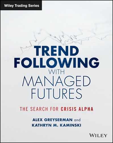
In the same autocorrelation study, they examine a comprehensive list of 793 CTAs. This large set of CTAs includes both trend followers and nontrend followers. For each CTA in the sample, the first five autocorrelation coefficient estimates are summed up. For each CTA, the correlation with the mini-trend index (including five well-established trend following managers) is also estimated. Figure 17.4 first ranks the first five autocorrelation lags (a measure of negative serial autocorrelation) and compares this rank with the correlation to trend following (via the mini-trend index). Roughly the first 100 CTAs on the left-hand side have both high ranking for serial autocorrelation and high correlation with the mini-trend index. The main concept is that these managers are most likely trend following CTAs. The property of negative serial autocorrelation seems to be a general characteristic of trend following managers as a class.
FIGURE 17.3 Autocorrelation coefficients 1 to 5 (ACF-1 to ACF-5) for the mini-trend index (Mini Sub Index) and the five managers in the index.
Source: Barclay Hedge and Newedge Investment Solutions.

FIGURE 17.4 Upper panel: Serial autocorrelation effects (sum of the first five correlation coefficients for 793 CTAs). Lower panel: Correlation with the mini-trend index (a small index of five well-established trend following CTAs).
Source: Barclay Hedge, Newedge Alternative Investment Solutions.
The previous discussion of serial autocorrelation was based on actual track records. A theoretical view of serial autocorrelation may provide some confirmation or discussion. Fung and Hsieh (2001) demonstrate how trend following strategies can be replicated by a portfolio of lookback straddle options. If a lookback straddle option strategy is assumed to represent trend following performance over time, this strategy can be examined for mean reversion using a variance ratio test. The closed form expression for the lookback straddle option strategy allows for a closed form expression for the variance ratio statistic. A variance ratio statistic is the ratio between the variance of an n-time-unit (n > 1) aggregated change and n times of the variance of single-time-unit change. A variance ratio statistic of 1 indicates a random walk. When the variance ratio statistic is below 1, a time series is mean reverting. Under certain conditions in Greyserman (2012), the variance ratio statistic for the lookback straddle option strategy can be shown to be lower than 1, indicating that trend following return series may exhibit mean reversion. Given the highly technical nature of variance ratio statistics and lookback straddle options, details are discussed in the appendix of this chapter.
variance ratio statistic the ratio between the variance of an n-time unit (n > 1) aggregated change and n times the variance of single-time-unit change. The variance ratio statistic can be used to test for deviations from a random walk.
Performance of Momentum Seeking
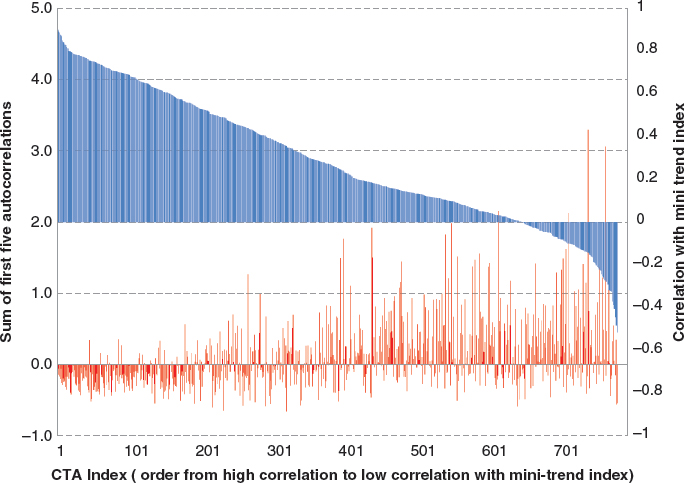
If trend following returns are mean reverting, momentum seeking approaches for dynamic allocation to trend following should underperform. To examine an extreme case, trend following rules can be applied to dynamically allocate to a trend following program (the trend following squared approach). To demonstrate the performance of trend following a trend follower, trend following return series are fed back into a trend following system with a short-sales restriction. Unlike futures positions, it is only possible to invest in a trend follower. Short selling is not possible for funds. To examine the potential for using trend following squared as a method to dynamically allocate to trend following, a generic trend following system with a Sharpe ratio of 0.94 is examined.1 It is important to remember that the Sharpe ratio of 0.94 comes from a buy-and-hold investment in trend following over the entire sample period. Trend following squared involves trying to find trends in trend following performance and allocating based on these trends. Figure 17.5 plots the Sharpe ratio for trend following squared as a function of the lookback window size for trend following a trend follower. Figure 17.3 demonstrates that, regardless of the chosen parameter (the lookback size), trend following squared (TF^2) never outperforms the buy-and-hold trend following portfolio with a Sharpe ratio of 0.94. The performance of a momentum seeking approach such as trend following squared demonstrates how improper dynamic allocation approaches can deteriorate performance.
FIGURE 17.5 Sharpe ratios for trend following squared allocation strategies when applied to a representative trend following.
Performance of Dynamic Allocation Strategies
Empirical evidence suggests that trend following return series exhibit negative serial autocorrelation. If this is the case, mean reversion strategies should potentially perform in line or possibly even better than a buy-and-hold strategy, and especially better than momentum seeking strategies. For a simple example, a buying-at-the-dips (or buying in a drawdown) approach might have some merit. A buying-at-the-dips approach increases allocation when the strategy is in a drawdown. On the other hand, if return series are sufficiently noisy, it may be too difficult to determine when or if a true drawdown is occurring. In this situation, a buy-and-hold investment may still be more prudent than a buying-at-the-dips approach.
A strategy that buys at the dips is somewhat similar to Martingale betting. As discussed in Chapter 9, dynamic leveraging can be used to elevate Sharpe ratios while exposing an investor to the increased risk of a large tail event. This type of event is magnified by the higher leverage in conjunction with the continuation of the drawdown. In this section, mean reversion in trend following returns enhances Sharpe ratios for investors who buy-at-the-dips. For the cases when the maximum leverage is capped for buying-at-the-dips, the total expected return can be lower while the risk of extreme losses is held somewhat in check.
To examine if a buying-at-the-dips strategy would improve on a buy-and-hold portfolio, a simple experiment can be applied. Assume an investor buys and holds an allocation of x percent in trend following. For the remaining (100 − x) percent, the investor increases investment in the trend following portfolio when the performance is down, buying-at-the-dips, and reduces investment when the performance is up, taking profits. Even more specifically, the change in investment is proportional to the strength of a trend signal based on cumulative trend following returns. The investor increases (reduces) allocation linearly to the portfolio when the downtrend becomes stronger (weaker). This means that when a drawdown is larger the allocation will be larger.
For allocations between 0 and 100 percent, Figure 17.6 plots the Sharpe ratios for the combined total portfolio return with x percent in buy-and-hold and (100 – x) percent using a buying-at-the-dips approach. To demonstrate how this approach would work, assume that an investor wants to invest $200M to trend following with 50 percent of the allocation in a passive, buy-and-hold approach. The investor invests $100M in trend following buy-and-hold. When the trend signal for the cumulative trend following return becomes negative, the investor starts to add to the system from the remaining $100M budgeted for investment. When the negative signal reaches the maximum strength, the $100M will be completely invested in the system and the total investment becomes $200M. When the trend signal becomes positive, the total investment will be reduced back to the original $100M allocated. Using this mean reverting dynamic allocation scheme, the investor would achieve a Sharpe ratio of above 1.0. Despite the fact that this strategy allocates less than all of the capital, it performs with a Sharpe ratio above the buy-and-hold Sharpe ratio of 0.94. As the amount of capital allocated to the passive buy-and-hold approach decreases the overall Sharpe ratio increases somewhat linearly.2
FIGURE 17.6 Sharpe ratios for a combined dynamic allocation trend following portfolio with x percent buy-and-hold (the horizontal axis) and (100 − x) percent buying-at-the-dips. (x) ranges from 0 percent to 100 percent.

Using Sharpe ratios as a measure for performance, an investor may be able to improve performance by timing allocations properly and buying-at-the-dips. When an investor combines a buy-and-hold allocation of x percent and a buying-at-the-dips allocation of (100 − x) percent, this is a form of dynamic leveraging. More importantly, in this case, the maximum leverage is restricted to the leverage employed by the buy-and-hold approach. This means that the leverage of the combined portfolio is often lower than, and never higher than the constant leverage employed by the buy-and-hold approach. It is also important to note that the buying-at-the-dips strategy is not always fully invested meaning that there are opportunity costs to underinvestment.
Buying-at-the-dips is a dynamic leveraging approach. In this study, it is bounded to make sure that it does not allow maximum leverage to exceed the leverage of a buy-and-hold approach. This reduces the probability of extreme losses.
In this example, a cap on the total leverage avoids the risk of large losses for accelerated dynamic leveraging schemes (for example Martingale betting). To demonstrate this effect, if the total allocation was allowed to exceed 100 percent, this leveraging scheme may provide drastic improvements in Sharpe ratio but at the risk of extreme drawdowns when leverage accelerates too quickly during a drawdown. Given the need to cap leverage for a portfolio that buys at the dips, an investor may expect an improved risk-adjusted return (the Sharpe ratio) at the cost of a reduced total expected return. When serial autocorrelation in trend following returns is sufficiently negative, a buying-at-the-dips approach may be able to improve return. The analysis in this section has demonstrated that both the level of mean reversion and overall risk reward tradeoffs (as measured by Sharpe ratios) can impact when mean-reverting approaches for dynamic allocation may be appropriate. The following section discusses this in more detail.
■ Investigating Dynamic Allocation Strategies
In the first section of this chapter, both serial autocorrelation and Sharpe ratios represent two statistical properties of returns that may help to classify when dynamic allocation is appropriate. Serial autocorrelation provides some indication of when returns exhibit persistence or mean revert. When Sharpe ratios are lower, dynamic allocation may be more desirable as performance may tend to occur in certain periods. When Sharpe ratios are high and serial autocorrelation is low, a passive buy-and-hold investment strategy is appropriate. When returns mean revert and Sharpe ratios are low, a buying-at-the-dips approach can make sense. When returns exhibit momentum and Sharpe ratios are low, a momentum-seeking approach can make sense. Logically, these conclusions are intuitive but in practice estimates for serial autocorrelation and Sharpe ratios are point estimates and often noisy ones. Because both Sharpe ratios and serial autocorrelations interact, optimal allocation strategies can be discussed more explicitly by examining the joint distribution of serial autocorrelation and Sharpe ratios.
To examine the performance of dynamic allocation strategies, an autoregressive AR(5) model can be used to generate return series. This model is selected to mimic the results from the Newedge whitepaper (2012), which demonstrates mean reversion for up to five months. The performance of dynamic allocation strategies can be estimated by Monte Carlo simulation. By ranging the serial autocorrelation and Sharpe ratio of returns in the AR(5) model, a wide range of scenarios for trend following returns can be examined. Beginning with a buying-at-the-dips approach, Table 17.1 displays the average return difference between buying-at-the-dips and buy-and-hold. For example, if the correlation is –0.16 and the Sharpe ratio is 0.4 the average return difference is 3.14 percent. Consistent with intuition, when the serial autocorrelation is negative and the Sharpe ratio is low, buying-at-the-dips outperforms buy-and-hold. When the serial autocorrelation is positive, buying-at-the-dips underperforms buy-and-hold. The results for momentum seeking are also consistent; when there is positive serial autocorrelation and a low Sharpe ratio, momentum seeking can outperform buy-and-hold.
TABLE 17.1 Average total return difference between buying-at-the-dips and buy-and-hold. Serial correlation ranges from –0.2 to 0.1 and the original Sharpe ratio is between 0.1 and 1.
| −0.2 | −0.18 | −0.16 | −0.14 | −0.12 | −0.1 | −0.08 | −0.06 | −0.04 | −0.02 | 0 | 0.02 | 0.04 | 0.06 | 0.08 | 0.1 | |
| 0.1 | 5.21 | 4.84 | 4.76 | 3.51 | 2.98 | 2.97 | 2.04 | 1.43 | 0.55 | −0.12 | −0.69 | −2.18 | −3.22 | −4.68 | −5.72 | −6.69 |
| 0.2 | 4.81 | 4.30 | 3.80 | 3.21 | 2.68 | 2.20 | 1.54 | 1.07 | 0.20 | −0.99 | −1.55 | −2.30 | −3.91 | −5.74 | −6.39 | −8.78 |
| 0.3 | 4.26 | 4.41 | 3.21 | 3.20 | 2.16 | 1.32 | 0.93 | −0.03 | −0.78 | −1.52 | −2.95 | −4.17 | −4.83 | −7.43 | −8.79 | −11.53 |
| 0.4 | 3.84 | 3.72 | 3.14 | 1.91 | 1.73 | 0.96 | −0.31 | −0.69 | −1.60 | −2.20 | −3.66 | −4.60 | −6.43 | −8.37 | −9.45 | −12.29 |
| 0.5 | 3.50 | 2.56 | 2.46 | 1.44 | 0.92 | 0.26 | −0.93 | −1.57 | −2.73 | −3.85 | −5.12 | −5.47 | −7.94 | −10.29 | −12.71 | −14.22 |
| 0.6 | 3.15 | 2.08 | 1.66 | 0.72 | 0.24 | −0.46 | −1.38 | −2.35 | −2.91 | −3.74 | −5.54 | −7.29 | −9.09 | −12.10 | −13.22 | −19.80 |
| 0.7 | 1.97 | 1.57 | 0.84 | 0.32 | −0.52 | −1.20 | −1.65 | −3.30 | −4.21 | −5.66 | −6.79 | −8.27 | −11.04 | −13.52 | −15.31 | −19.41 |
| 0.8 | 1.14 | 1.35 | −0.05 | −0.27 | −1.66 | −2.42 | −3.27 | −3.71 | −5.77 | −6.45 | −8.79 | −9.76 | −11.37 | −14.06 | −17.87 | −24.18 |
| 0.9 | 1.08 | 0.41 | −0.72 | −1.16 | −2.18 | −3.47 | −4.40 | −4.65 | −6.31 | −7.37 | −9.33 | −11.48 | −13.34 | −15.64 | −20.86 | −24.28 |
| 1 | 0.46 | −0.81 | −1.34 | −1.99 | −2.84 | −3.99 | −5.51 | −6.16 | −7.82 | −9.20 | −11.31 | −13.08 | −15.54 | −19.53 | −23.57 | −28.00 |
For a range of combinations of Sharpe ratios and serial autocorrelation, Table 17.2 illustrates four scenarios for dynamic allocation (including buy-and-hold) and the corresponding favorable return profiles for their application. Based on simulation, and for the range of examples, the results from simulation mirror the intuition for both buying-at-the-dips and performance-chasing. Allocation approach D, redeeming-in-a-drawdown, is a specific type of momentum-seeking strategy that redeems in a drawdown; the mirror opposite of the buying-at-the dips approach, which allocates in a drawdown.
TABLE 17.2 Four scenarios for dynamic allocation and the corresponding favorable return profiles for their application.
| Allocation Approach | Sharpe Ratios | Serial Autocorrelation | Example | |
| A | Buy-and-hold | High | Low | Shp > 0.8,|ρ| < 0.1 |
| B | Buying-at-the-dips | Low | Negative | Shp < 0.3,ρ < −0.1 |
| C | Performance-chasing | Low | Positive | Shp < 0.3,ρ > 0.1 |
| D | Redeeming-in-a-drawdown | High | Positive | Shp > 0.8,ρ > 0.1 |
The most effective investment approach depends on the joint distribution of the return’s Sharpe ratio and serial autocorrelation.
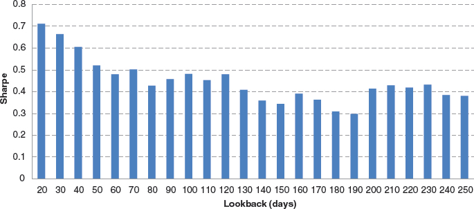
Returning again to the buying-at-the-dips allocation approach, a return profile similar to the point estimates for actual trend following return series can be examined more closely. Using a return generating process with a Sharpe ratio of 0.9 and slightly negative serial autocorrelation, the performance of the buying-at-the-dips strategy can be examined as a function of the amount x percent that remains buy-and-hold. For a given Sharpe ratio of 0.9 and slightly negative serial autocorrelation, Figure 17.7 plots the total return for a combined portfolio with x percent buy-and-hold and (100 − x) percent buying-at-the-dips. Similar to the previous example with buying-at-the-dips, the total capital, or the maximum capital invested in the trend following program, is the same for all allocation percentages (x). Maximum leverage is capped at the same level for a 100 percent buy-and-hold portfolio. Figure 17.7 demonstrates Scenario A where a buy-and-hold allocation should be a favorable strategy. In the case where the serial autocorrelation is only slightly negative and the Sharpe ratio is high, buying-at-the-dips reduces the performance of a buy-and-hold strategy. More specifically, when the strategy has half of its capital in buy-and-hold (x = 50 percent), the total return is reduced from 13 percent to roughly 8 percent if the investor nothing.
FIGURE 17.7 Scenario A: The total return of combining buy-and-hold x percent (the horizontal axis) and buying-at-the-dips (100 − x) percent, with (x) varying from 0 to 100, to a representative trend following system.
On the other hand, for periods when the Sharpe ratio is sufficiently low and serial correlation is negative, the opposite may be true. This is a Type B scenario where buying-at-the-dips may outperform buy-and-hold. Using a return generating process with a low Sharpe ratio and more negative serial autocorrelation, Figure 17.8 plots the total return for a combined portfolio with x percent buy-and-hold and (100 − x) percent buying-at-the-dips. Because Sharpe ratios are lower, overall returns are lower. In a Type B scenario, a reduction in the amount allocated to buy-and-hold in favor of buying-at-the-dips increases performance linearly.
FIGURE 17.8 Scenario B: The total return of combining buy-and-hold x percent (the horizontal axis) and buying-at-the-dips (100 − x) percent, with (x) varying from 0 to 100, to a representative trend following system.

Optimization with Uncertainty
Sharpe ratios and serial autocorrelation are not deterministic. Even more complicated, they are not independent of each other typically following a joint statistical distribution. The classifications for Type A and Type B scenarios are somewhat broad. From the investor’s perspective, it would be ideal to have a method for determining (x), or the percentage that should remain in buy-and-hold. This problem is a classic problem of optimization under uncertainty. The objective is to maximize the total expected return using a penalty for uncertainty.3 When an investor is relatively confident about the point estimates for the Sharpe ratio and serial correlation, the weight for the penalty item can be insignificant. In this case, the optimum solution will be either 100 percent Type A or Type B. On the other hand, when an investor is less confident with the point estimates for the Sharpe ratio or serial autocorrelation, the uncertainty penalty should be large. The optimal solution is the x that makes the distribution of total expected return as uniform as possible across a range of possible values for the “true” Sharpe ratio and serial correlation.
Because of the uncertainty related to the joint distribution of Sharpe ratio and serial correlation, the optimal approach is usually a combination of two investment approaches.
Optimization under uncertainty can be rather complex and heuristic solutions often provide rather robust solutions to these types of problems.4 Intuitively, given uncertainty regarding the return distribution, the optimal solution can be estimated heuristically as the average value for x over a range of possible range of distributions for the Sharpe ratio and serial autocorrelation. For a specific example, a typical trend following program with serial autocorrelation of –0.1 and a Sharpe ratio distributed uniformly between 0.3 and 0.8 can be considered. In this case, the best solution is 50 percent buy-and-hold and 50 percent buying-at-the-dips. This result is based on the results in Table 7.1. As another example, imagine a scenario when an investor is more positive about the Sharpe ratio, perhaps between 0.5 and 0.8, and he/she estimates the serial autocorrelation between –0.12 and –0.08. The best solution would be 75 percent buy-and-hold and 25 percent buying-at-the-dips.
Reflections on Dynamic Allocation
For periods of mean reversion in performance, the buying-at-the-dips approach has been shown to increase the performance of buy-and-hold. This conclusion may raise the question of whether trend following managers themselves should consider incorporating this into their approach. There are several issues with this conclusion. First, trend following managers may consider it suboptimal to select a structured point of x percent. Second, the investors’ and trend following managers’ views on Sharpe ratios and serial autocorrelation may differ substantially creating a mismatch in expectations. Investors and managers may also have different objectives. For example, an investor interested in high crisis alpha may be less concerned with total return as an objective. Another investor who uses a risk parity approach may also have a completely different objective than total portfolio return.
Despite many complications, there is one important message from this analysis. Dynamic allocation strategies should only be applied when there is sufficient evidence that trend following returns exhibit the proper return characteristics. The corresponding level of uncertainty regarding the underlying return characteristics for trend following returns point to either a buy-and-hold approach or buying-at-the-dips. An investor who is confident in long-term performance expectations (i.e., a Sharpe ratio close to 1) should size the initial investment according to expected drawdown risks and follow a buy-and-hold approach.5 An investor, who is less confident about performance expectations, should maintain a significant level of baseline buy-and-hold investment (for example, 50 to 75 percent) and deploy the remaining capital buying-at-the-dips. This mean reversion strategy accumulates exposure during dips in performance and reduces exposure following a significant increase in performance. For one final point, this analysis also provides a word of caution for performance chasing. Performance chasing is not compatible with the mean reverting nature of trend following returns.
Different investors may have a range of views on the distribution for the Sharpe ratio and serial correlation as well as different objectives. As a result, optimal allocation to buying-at-the-dips is investor specific.
■ Summary
Once an investor has decided to invest in trend following strategies, the next natural question is how and when. Dynamic allocation approaches can be divided into three types: buy-and-hold, momentum seeking, and mean reversion. The choice of dynamic allocation strategy should directly depend on the underlying statistical properties of trend following returns. Empirical evidence provides support for mean reversion in trend following performance. Despite this evidence, it is also necessary to take the level of risk in returns and Sharpe ratios into account. This chapter examined the buying-at-the-dips approach to dynamic allocation in comparison with a simple buy-and-hold. Using joint distributions for the Sharpe ratio and serial autocorrelation in returns, a number of scenarios for favorable environments for different allocation approaches can be summarized. Buy-and-hold strategies are the most favorable when the Sharpe ratio is high and absolute levels of serial autocorrelation are low. Mean reverting strategies, such as buying-at-the-dips, are the most favorable when Sharpe ratios are lower and serial autocorrelation is negative. Momentum strategies, such as performance chasing, are the most favorable when Sharpe ratios are lower and serial autocorrelation is positive. Given the empirical and theoretical evidence for trend following returns, dependent on the investor’s objectives and risk tolerance, the appropriate dynamic allocation approach varies between buy-and-hold and buying-at-the-dips. Given the analysis in this chapter, a word of caution is also extended for performance chasing trend following: dynamic allocation approaches of this type can reduce performance substantially.
■ Appendix: A Theoretical Analysis of Mean Reversion in Trend Following
Earlier in this chapter, mean reversion in trend following return series was a key factor in determining which dynamic allocation could be appropriate for an investor and when. This section turns to a theoretical analysis of serial autocorrelation properties and variance ratio statistics. Under the assumption that trend following returns are replicated by lookback straddle options from Fung and Hsieh (2001), it is possible to express the PnL as a function of the change in price of the lookback straddle price. Under certain simplifying assumptions, Greyserman (2012) demonstrates that the price change of a lookback straddle can be shown to be mean reverting using the variance ratio statistic (Lo and MacKinlay 1988). This appendix reviews the variance ratio statistic and the lookback straddle option for replicating trend following from Fung and Hsieh (2001).
Mean Reversion and the Variance Ratio Statistic
If a time series follows a random walk, the variance of the n-time-unit aggregated change is n times of the variance of single-time-unit change, as shown in the following equation:

where V(n) is the variance ratio statistic between δn2, the variance of the n-time-unit aggregated change (n > 1), and n times δ12, the variance of single-time-unit change. The variance ratio test is one of the standard statistical tests for a random walk (Lo and MacKinlay 1988). This section is not focused on testing the statistical significance of a time series being a random walk. Instead this section is focused on the variance ratio’s link to mean reversion. Negative serial correlation corresponds to a variance ratio statistic lower than 1.6 Given this fact, return series can be loosely defined as mean-reverting when the variance ratio statistic is lower than 1. Figure 17.9 presents a schematic for price processes, strategies, and variance ratio statistics.
FIGURE 17.9 A schematic for price processes, strategies, and variance ratio statistics.

To demonstrate this empirically, Figure 17.10 plots two time series with a serial autocorrelation of 0.3 and –0.3 of per unit time change respectively. From this example, the time series with the negative serial autocorrelation appears to exhibit more mean reversion than the one with positive serial autocorrelation. In this example, the variance ratio statistic V (2) for the time series with positive serial autocorrelation is 1.25, while V (2) for the time series with negative serial autocorrelation is 0.70. This example demonstrates the link between serial autocorrelation and the variance ratio statistic.
FIGURE 17.10 Sample time series for two series with serial autocorrelations of 0.3 and –0.3 respectively.

Trend Following and the Lookback Straddle Option
From a theoretical perspective, Fung and Hsieh (2001) established the equivalence of trend following and holding lookback straddle options. The performance of the lookback straddle option was discussed in Chapter 13. In this chapter, in comparison with other manager-based indices and price-based trend indices, the lookback straddle option seemed to exhibit the poorest fit in a return-based style analysis. This may demonstrate the subtle difference between position taking and option strategies. Due to the importance of the lookback straddle in the trend following literature, it is discussed further here. According to Goldman, Sosin, and Gatto (1979), the price of a lookback call option with time to maturity (T) at time t (t < T ), can be expressed using the following formula:

where τ = T − t, r is the continuously compounded risk-free rate, St is the underlying market price at time t, σ is the underlying market volatility (assumed to be constant), Qt is the lowest price for the underlying market up to time t, and N(⋅) is the standard normal cumulative distribution function. In addition, let

Similarly, the price of a lookback put option at time t is expressed as follows:

where Mt is the highest price of the underlying market up to time t. The price of a lookback straddle at time t is then simply LCt + LPt. Correspondingly, the profit and loss (PnL) of a trend following portfolio is proportional to the change in LCt + LPt.
The PnL of trend following in a given period can be expressed in the price change of a lookback straddle option.
■ Further Readings and References
Cukurova, S., and J. Martin. “On the Economics of Hedge Fund Drawdown Status: Performance, Insurance Selling and Darwinian Selection.” Working paper, 2011.
Fung, W., and D. Hsieh. “The Risk in Hedge Fund Strategies: Theory and Evidence from Trend Followers.” Review of Financial Studies 14, no. 2 (2001).
Greyserman, A. “The Fallacy of Trend Following Trend Following.” ISAM white paper, November 2012.
Goldman, M., H. Sosin, and M. Gatto. “Path Dependent Options: ‘Buy at the Low, Sell at the High.’” Journal of Finance 34, no. 5 (1979).
“It’s the Autocorrelation, Stupid.” Newedge white paper, November 2012.
Lo, A., and A. MacKinlay. “Stock Market Prices Do Not Follow Random Walks: Evidence from a Simple Specification Test.” Review of Financial Studies 1, no. 1 (1988).
1 This trend following strategy is examined from 1993 to 2012.
2 The return is based on the total maximum allocation. The uninvested capital is assumed to be in cash with zero return. Transaction costs as well as subscriptions and redemption costs are excluded from this analysis.
3 When the penalty item is the variance of the expected total return over the set of possible values for the Sharpe ratio and serial correlation, the optimization is similar to the classical mean variance optimization. In this case, the variance here is not the portfolio return variance.
4 The field of robust optimization provides alternative methods for performing optimization when there is uncertainty in the distribution of underlying parameters. This section resorts to a heuristic method for estimating the optimal solution for such an optimization problem.
5 For a comprehensive discussion of drawdown characteristics, see Chapter 8.
6 The opposite case is that, when the serial correlation is positive, the variance ratio is larger than 1, indicating momentum in the time series.