CHAPTER 14
Portfolio Perspectives on Trend Following
Up until this point, trend following has been examined somewhat in isolation. The remainder of this book turns to trend following from a more global perspective. This chapter reviews three core issues that represent advanced topics: the role of equity markets and crisis alpha, understanding cyclicality in trend following volatility, and the role of mark-to-market for manager-to-manager correlations. This chapter opens the discussion of trend following from an investor perspective. Chapter 15 discusses the role of size, liquidity, and capacity. Chapter 16 examines the act of diversifying away from pure trend following. Chapter 17 discusses dynamic allocation to trend following across time.
■ A Closer Look at Crisis Alpha
Chapter 4 introduced the concept of crisis alpha in the context of adaptive markets. Throughout the following chapters the importance of crisis alpha is discussed using an array of measures and across construction styles for trend following. For an institutional investor, crisis alpha is a key characteristic for understanding how trend following strategies can perform during difficult periods for traditional portfolios. Chapter 7 discussed how crisis alpha can be applied for different asset classes. This section focuses on diving deeper into how equity markets relate to crisis alpha.
Equity Dependence
A typical trend following portfolio consists of seven sectors: equity indices, bonds, short-term interest rates (STIR), foreign currencies (FX), agriculturals, energies, and metals. Figure 14.1 plots the respective sector Sharpe ratios for a representative trend following system from 1999 to 2012.1 This sample period is chosen intentionally as the total buy-and-hold return for equity markets during this time period is approximately zero. Concurrently, trend following performance has been the weakest in the equity sector.2 To further examine the level of market divergence for each sector, the market divergence index (MDI) can be calculated at the portfolio level for each sector. When the MDI is greater than a threshold of 0.1, this indicates a period of higher divergence. For the specific case of equities, the probability that the sector MDI is greater than 0.1 can be used to measure the prevalence of trend following opportunities. As seen in Chapter 3, 0.1 is used as a threshold for a trend following portfolio as this is the MDI level where the system tends to have nonnegative performance on average. If the MDI is high, the signal-to-noise ratio for prices in that sector was high often indicating profitability for trend following strategies. Figure 14.2 plots the estimated probability that each sector MDI is greater than 0.1 for the sample period of 1999 to 2012. Across all sectors, equity markets have the lowest probability of being above the threshold of 0.1. Some might hypothesize that equity markets are more “efficient” in relative terms due to increased competition. There is also ample academic literature, for example, Monoyios and Sarno (2002) asserting that equity indices exhibit mean reversion in the long term. It is not clear if underperformance in trend following equities is due to increased competition or the underlying lack of market divergence in equity markets as an asset class.
FIGURE 14.1 Sharpe ratios for each sector for a representative trend following system. The sample period is from 1999 to 2012.
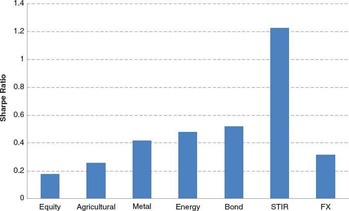
FIGURE 14.2 The estimated probability for each sector MDI being larger than 0.1. The sample period is from 1999 to 2012.

Crisis alpha is a simple measure of how a strategy performs during periods of market stress. Chapter 7 demonstrated how crisis alpha was related to performance across many sectors where equity market crisis is the stimulus. The sample period of 1999 to 2012 includes two extreme negative equity bear markets, yet equity markets exhibit the least divergence (or signal-to-noise ratios). This demonstrates how equity markets may be the instigator but clearly not the main source of crisis alpha.
Long- or Short-Equity Trends
Given that equity markets exhibit the least market divergence on a sector basis, this section examines the role of positive and negative equity trends. To examine directional effects in market divergence, it is possible to revisit the construction of the market divergence index (MDI) from Chapter 5. The signal-to-noise ratio is a ratio between the trend and individual price changes over a specific period. In order to measure the level of price divergence for a particular price series, the signal-to-noise ratio is used. For any specific day, at time (t), the signal-to-noise ratio (SNRt) for a particular price series with lookback period (n) can be calculated mathematically using the following formula:

where (Pt) is the price at time (t) and (n) is the lookback window for the signal, or the signal observation period. For medium- to long-term trend followers, this is typically chosen to be roughly 100 days. The MDI on day t is simply the average of (SNRit) for all markets in the portfolio. Based on historical data, when the MDI is above 0.1, markets are trend-friendly and on average positive returns are expected in the corresponding period.
When the absolute value is removed from the numerator for the signal-to-noise ratio, the result is a new market divergence index with signs (sMDI). When the sMDI is large and positive, this indicates a market environment with stronger uptrends. Figure 14.3 plots the estimated probability for each sector sMDI being larger than 0.1. Second only to fixed-income markets, equity markets have a high probability of having an sMDI greater than 0.1. Comparing Figure 14.2 and Figure 14.3, uptrends make up more than two-thirds of the periods when the MDI is higher than 0.1.3
FIGURE 14.3 The estimated probability for each sector sMDI being larger than 0.1. The sample period is from 1999 to 2012.

To examine directional equity positions only (long or short), the performances of a standard, a long-only, and a short-only trend following system can be compared. In this case, a long-only trend following system takes signals only in the long direction (flat or long), while a short-only trend following system takes signals only in the short direction (flat or short). Figure 14.4 plots the performance of these three systems from 1999 to 2013. By comparing these three systems, it can be observed that short positions in a standard symmetric trend following system contribute to substantially negative PnL. During this sample period, restricting short positions would have improved performance in the equity sector. Table 14.1 presents performance statistics for the equity sector across all three trend following systems: the standard symmetric trend following system, one with only long positions, and one with only short positions.
TABLE 14.1 Performance statistics for a standard symmetric trend following system, a system with long positions only, and a system with short positions only in the equity sector. The sample period is from 1999 to 2013.
Sharpe |
Return (monthly) (%) |
Risk (monthly) (%) |
|
| Standard | 0.36 |
0.80 |
7.52 |
| Long Only | 0.41 |
1.32 |
10.95 |
Short Only |
–0.07 |
–0.25 |
11.36 |
FIGURE 14.4 Cumulative performance for a standard symmetric trend following system, a system with long positions only, and a system with short positions only in the equity sector. The sample period is from 1999 to 2013.

For the sample period from 1999 to 2012, the long-only system has the highest Sharpe ratio. The long-only system has positive performance beginning in 2009. In contrast, the standard trend following system has remained down from 2009 to 2012. Despite the increase in Sharpe ratio, the trend following system, which is long only in equities, has negative skewness of –0.25 whereas the standard symmetric trend following system has positive skewness of 0.23. The shift in return skewness from positive to negative suggests that there are larger tail risks and possibly a less desirable risk profile for the long-only system in equities. This motivates a closer look at what happens in equity markets during extreme market events such as crisis.
Crisis Alpha
Crisis alpha is a measure of performance during periods of market stress. Using the VIX-based approach from Chapter 7, any month with a move in the VIX greater than 20 percent over the previous level of the VIX is labeled as a crisis month. Figure 14.5 displays the S&P 500 Index where the VIX based crisis periods are highlighted by the shaded bars.
FIGURE 14.5 The S&P 500 index from 1999 to 2013 with VIX-based crisis periods highlighted by the shaded bars.
Data source: Bloomberg.

Realistically, trend followers do not completely remove short-equity signals. Instead of examining long-only positions in the equity sector, a bias of 5:1 for long positions versus short positions is applied. Figure 14.6 compares the crisis alpha contribution for both the standard symmetric and long-biased (in the equity sector) trend following systems. It is important to note that equity is only one of the seven sectors of the whole portfolio. From Figure 14.6, the impact of removing short-equity signals from a trend following system increases total return by more than 1 percent. This restriction increases total return, but it comes at the cost of crisis alpha. Crisis alpha performance is reduced from roughly 5 percent to close to zero. More specifically, an improvement in the Sharpe ratio (from 0.77 to 0.86 for the whole portfolio) is at the cost of 4.6 percent crisis alpha.
FIGURE 14.6 A comparison of total return and crisis alpha, with a VIX-based crisis period definition, for both a standard symmetric trend following system and a trend following system with equity-long positions only. The sample period is from 1999 to 2012.

To demonstrate the robustness of this effect, a second definition for a crisis period can be used based on past returns. A crisis month can be defined as any month with a lower than minus 5 percent return for the S&P 500 Index. Figure 14.7 displays the S&P 500 Index with the returns-based crisis periods highlighted by the shaded bars. Figure 14.8 compares the crisis alpha contribution for both the standard symmetric and long-only (in the equity sector) trend following systems. Despite the different definition for crisis periods and change in index, the results are roughly the same. Removing short equity signals from a trend following system increases the total return at a corresponding cost in crisis alpha. From Figure 14.8, the net reduction in crisis alpha is approximately the same at 4.6 percent (from 8.7 to 4.1 percent).
FIGURE 14.7 The MSCI World Index with crisis periods, where crisis is defined by monthly returns less than minus 5 percent, highlighted by the shaded bars from 1993 to 2013.
Data source: Bloomberg.

FIGURE 14.8 A comparison of total return and crisis alpha, with an SPX return-based crisis period definition, for both a standard symmetric trend following system and a trend following system with equity-long positions only. The sample period is from 1999 to 2012.

Portfolio Effects of Long Equity Bias
The first part of this section demonstrated how equity-long bias comes at the cost of crisis alpha. To examine this effect from an investor’s perspective, the impact should also be examined at the total portfolio level. For simplicity, two institutional portfolios are considered in this analysis: the traditional 60/40 equity bond portfolio and a fund of funds (FoF) portfolio. The 60/40 portfolio can be examined using a 60 percent allocation to the MSCI World Index and 40 percent allocation to the JPMorgan Global Bond Index (GBI). The fund of funds portfolio will be represented by an allocation to the HFRI Fund of Fund Index (HFRIFOF). The hedge fund indices are not necessarily investable but their return series can represent how a fund of funds investor might have performed over time. Each of the institutional portfolios will be combined with a 20 percent allocation to trend following. The first combined portfolio consists of an 80 percent allocation to the 60/40 portfolio (48 percent stocks, 32 percent bonds) and 20 percent allocation to trend following. The second combined portfolio is an 80 percent allocation to the fund of funds index (HFRIFOF) and 20 percent in trend following.4
Table 14.2 displays the performance statistics for a traditional 60/40 portfolio when compared with adding trend following both with or without a long bias in equity positions.5 The standard symmetric trend following program has a larger increase in Sharpe ratio and larger reduction in maximum drawdown. Adding a long equity bias increases the average return more than the symmetric system. Table 14.3 displays the performance statistics for an institutional investor with a fund of funds allocation compared with adding trend following with or without long bias in equity positions. For the fund of funds investor, adding a long bias to a trend following program reduces both the average return and the Sharpe ratio.
TABLE 14.2 Performance statistics for both a 60/40 portfolio and a 60/40 portfolio combined with trend following. The total combined portfolio consists of 48 percent stocks, 32 percent bonds, and 20 percent trend following over a sample period from 1999 to 2012. The combined portfolio includes either a symmetric trend following program or a trend following program with long equity bias.
Sharpe Ratio |
Monthly Return (%) |
Monthly Volatility (%) |
Maximum DD (%) |
|
| Traditional Institutional (60/40) | 0.68 |
0.72 |
3.55 |
44.47 |
| With 20% Trend Following (Symmetric) | 0.94 |
0.80 |
2.86 |
24.97 |
| With 20% Trend Following (Long-Biased Equity Sector) | 0.91 |
0.82 |
3.02 |
27.57 |
Data source: Bloomberg.
TABLE 14.3 Performance statistics for both a fund of funds portfolio and a fund of funds portfolio combined with trend following. The total combined portfolio consists of 80 percent in the HFRIFOF and 20 percent trend following over a sample period from 1999 to 2012. The combined portfolio includes either a symmetric trend following program or a trend following program with long equity bias.
Sharpe Ratio |
Monthly Return (%) |
Monthly Risk (%) |
Max DD (%) |
|
| Fund of Funds Index (HFRIFOF) | 0.73 |
1.08 |
4.96 |
71.23 |
| With 20% Trend Following (Symmetric) | 1.23 |
1.54 |
4.25 |
22.97 |
| With 20% Trend Following (Long-Biased Equity Sector) | 1.12 |
1.18 |
3.56 |
19.84 |
Data source: Bloomberg.
In the first part of this section, long equity bias in a trend following portfolio was shown to increase total return and Sharpe ratios at the cost of crisis alpha. From the perspective of a trend following manager, this may be desirable. From the perspective of an institutional investor, when trend following programs are combined with common institutional portfolios, long equity bias decreases the Sharpe ratio for a total portfolio. For the 60/40 portfolio, removing the long bias is more effective for drawdown reduction. Although the results are somewhat mixed, there seems to be compelling evidence that long bias may be in the interest of the manager more than the interest of the investor.
■ The Impact of Mark-to-Market on Correlation
Correlation is undoubtedly one of the most commonly used quantitative measures to classify relationships between managers. Lower correlations between managers generally imply a diversification of styles and approaches. This typically leads investors to conclude that it is more beneficial to invest in a larger number of managers in a particular space. Given the reliance on correlation as a measure, it is highly important that correlation estimates are accurate. Turning to the futures industry, there is one particular technical aspect of futures trading that is often ignored, standardized mark-to-market for net asset value (NAV) calculation. This section demonstrates empirically how, for strategies without standardized mark-to-market on settlement prices, correlation may be understated. In simple terms, correlations in managed futures are high and appropriate. For managers outside of managed futures, correlations may be lower simply due to the lack of a standardized mark-to-market mechanism.
Mark-to-Market and Illiquid Markets
Several academic papers have illustrated the impact of illiquidity on hedge fund returns. For example, Getmansky, Lo, and Makarov (2004) provide strong evidence that mark-to-market or mark-to-model practice has caused high serial autocorrelation of hedge fund returns in most categories as a result of market illiquidity. One of the often overlooked impacts of illiquid markets is the impact on the correlation between managers (or funds). Mark-to-market or mark-to-model practice is a potential source of significant variation in settlement pricing in illiquid markets. This variation artificially decreases the correlations between managers trading these assets as they may adopt different settlement and pricing methods for the purposes of calculating returns and net asset value (NAV).
An important source of variation for mark-to-market pricing in less liquid markets is the simple bid-ask spread. Arakelyan and Serrano (2012) examine the bid-ask spread for various credit default swap (CDS) markets. To put bid-ask spreads outside of futures contracts into perspective, the average bid-ask spread for a one-year maturity CDS market, with a rating of BBB, is 13 bps with a standard deviation of 22 bps. A bid-ask spread of this magnitude is often of the same order of magnitude as the daily volatility of CDS markets. For futures markets, the bid-ask spreads are considerably lower. Across the industry, standardized settlement prices are used to mark-to-market positions daily regardless of bid-ask spreads.
Liquidity and Correlation
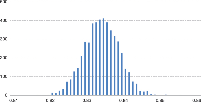
For illustrative purposes, a simple scenario can be used to explain the potential impact of the bid-ask spread on correlation. First, consider a situation with two identical managers. In this case, both managers have the same return series and their correlation is 1. Next, variations between these identical managers can be imposed by adding a bid-ask spread to the original returns. This can be achieved by modeling a certain spread distribution. Instances of this distribution are chosen randomly for a mark-to-market price within the bid-ask distribution. Figure 14.9 shows the histogram of correlations between the identical manager returns after the assumed bid-ask spread has been added. In this example, the average bid-ask spread is set as 20 percent of the daily volatility for the original return series and the standard deviation of the bid-ask spread is set at 40 percent of the daily return volatility. In this example on average the correlation drops from 1 to 0.8. This example shows how the addition of variation in the bid-ask spread can reduce correlation (even if return series are perfectly correlated). In many less liquid security markets (i.e., the credit space), the bid-ask spread can be even larger than the one used in the example.
FIGURE 14.9 The distribution of the correlation between two return series (perfectly correlated) after the assumed bid-ask spread is added.
In the CTA industry, managers may have correlations as high as 80 percent. For two CTA managers with an 80 percent correlation, without mark-to-market and standardized settlement prices, the observed correlation can be as low as 50 percent. These examples show how simple variations in bid-ask spread and mark-to-market may potentially decrease correlations. Put in another way, the lack of standardization and consistent mark-to-market mechanism reduces correlations between managers. To examine how this relates to managed futures, variation in mark-to-market and its relation to intermanager correlations is examined in greater detail in the following section.
Mark-to-Market and Trend Following
The previous section demonstrated how illiquidity and variations in the bid-ask spread may understate correlation between managers. This section examines two highly correlated representative trend following systems trading a diversified universe of liquid futures markets. Over the past 20 years, the correlation between the daily returns of these two trend following systems is 0.96.
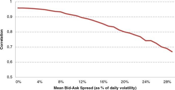
As explained earlier in this section, managed futures funds trade mostly liquid futures markets, which provide the daily settlement price at the exchange. As a result, there is no need for a discretionary decision in the mark-to-market methodology. However, to demonstrate the possible impact of mark-to-market variability, the variation of mark-to-market pricing is simulated by imposing a statistical price distribution around the daily settlement price. Instances for the price series are sampled to set the mark-to-market calculation of daily PnL. It is important to note that this noise is added for the PnL calculation only. The signals and positions for the underlying systems are not impacted in any way. Daily returns for various assumed bid-ask spreads are expressed as a percentage of the daily price volatility for each market. Figure 14.10 shows the correlation between the two highly correlated trend following funds as a function of the average bid-ask spread for mark-to-market. For a specific example, when the mean bid-ask spread is assumed to be 20 percent of the daily price volatility, the impact of this variation on the daily settlement price reduces correlation from 0.96 to 0.8, a reduction of 17 percent in correlation. From an investor perspective, without standardized mark-to-market for daily settlement prices, these highly similar managers look seemingly more dissimilar.
FIGURE 14.10 The correlation between the daily returns of two trend following systems at various assumed mean bid-ask spread as a percentage of the volatility of daily price changes.
The important takeaway from this example is that if trend following strategies did not mark-to-market by daily settlement prices set by the exchange, they would have substantially lower correlations between managers. This means that many other strategies, which they are often grouped with, in the alternative space may have understated intermanager correlation. The lack of a standardized mark-to-market mechanism can augment their potential value for diversification.
■ Understanding Volatility Cyclicality
Volatility is an important part of risk taking and understanding risk over time. In practice, volatility is not constant but time varying. This concept especially holds true for dynamic trading strategies. One way to examine how volatility changes over time is to look at volatility cyclicality. Volatility cyclicality is defined as the relative speed of cycles in volatility for a particular trading strategy. If a strategy is relatively slow over time, volatility cycles should be low frequency. This means that a period of a volatility cycle is perhaps as long as a year. Volatility in trend following is time varying and it tends to exhibit lower cyclicality. On the other hand, for aggressive position taking approaches where volatility quickly accelerates and decelerates, this exhibits high cyclicality in volatility. As discussed in Chapter 9, dynamic leveraging is a perfect example of an approach that should cause high-frequency volatility cycles. A closer look at option selling strategies and Martingale betting in Chapter 9 demonstrated spikes in volatility and high cyclicality in volatility patterns. As a review, dynamic leveraging is defined as a situation where the amount of leverage depends on the past profits and losses (PnL) of the portfolio. In simple terms, a dynamically leveraged portfolio, which increases (or decreases) its bet size when there are many past losers (or past winners), engages in dynamic leveraging. Dynamic leveraging is similar to “doubling down” in poker. Chapter 9 discussed how dynamic leveraging can include hidden leverage risk in Sharpe ratios.
volatility cyclicality the relative speed of cycles in volatility for a particular trading strategy. This can be measured by examining frequencies in the spectral representation of a time series.
Volatility cyclicality can be examined more directly using spectral analysis. Practically, Fourier transforms can be used to extract and identify volatility cycles. A Fourier transform converts a signal from the time domain to the frequency domain allowing for both the identification and filtering of volatility cycles.6 The Fourier transform can be applied to 22-day (approximately one month) rolling volatilities to reveal the corresponding high and low frequency components.7 Periods are plotted as a function of their power (strength), which can be plotted as a periodogram.8 More specifically, a periodogram is the spectral density of a signal; it power weights the frequencies by their importance in a signal. To begin the discussion of volatility cyclicality of trend following, Figure 14.11 plots the periodograms for trend following (Newedge Trend Index) and equity markets (MSCI World Index). The periodogram of the trend following index shows no obvious dominant frequency corresponding to a period shorter than 252 days. In contrast, the periodogram for the 22-day rolling volatility of the equity index shows several dominant higher frequencies. Figure 14.11 demonstrates that volatility cycles in trend following are longer and perhaps smoother then volatility cycles in equity markets. A simple spectral analysis of trend following and equity markets demonstrates how, in contrast with equity markets, the volatility adjustment for positions in trend following is able to smooth out the cyclical effects in volatility over time. The volatility adjustment for trend following was introduced in Chapter 3 and explained in further detail in Chapter 8.
FIGURE 14.11 The periodograms of higher frequency components for the 22-day rolling volatility of the Newedge Trend Index and the MSCI World Index.

Extracting Dynamic Leveraging from Manager Performance
The previous section introduced the concept of cyclicality in volatility. A view over both low and high frequencies demonstrated that trend following exhibits lower cyclicality in volatility than equity markets. In contrast to looking at volatility cyclicality over lower frequencies, this section returns to the discussion of dynamic leveraging and the impact of high-frequency volatility cycles. In practice, spikes and high cyclicality in volatility patterns is a signature of dynamic leveraging. Trend following systems are not designed to accelerate positions as a function of PnL. Returning to the example in Chapter 9, Martingale betting is an example of a dynamic leveraging scheme that can boost Sharpe ratios. As a review, Martingale betting works in the following way: when faced with a loss, the long position is increased until the first day of positive PnL. Bets are increased when they are losing (another form of doubling down). If Martingale betting is applied to a trend following system, the number of double-down days must be limited to remain tractable.
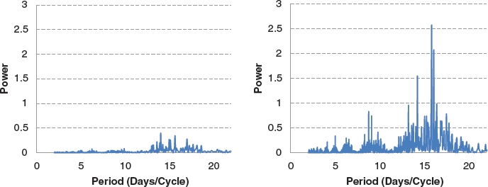
Dynamic leveraging is similar to “doubling down” in poker. Aggressive patterns in the application of leverage can be isolated in a manager return series. This allows an investor to determine at which level dynamic leveraging may potentially be inflating Sharpe ratios. Again for the case of high-frequency effects, Fourier transforms can be used to extract and identify volatility cycles. To demonstrate the power of a Fourier transform in extracting dynamic leveraging effects, Figure 14.12 displays the periodograms for only the high-frequency components for the 22-day rolling volatility of the representative trend following system (left panel) and the system with limited Martingale betting (right panel). The periodogram of the representative trend following system shows no dominant frequency corresponding to a period less than 22 days. In contrast, the periodogram for the 22-day rolling volatility with limited Martingale betting shows several dominant frequencies. The strength of these high-frequency effects represents the accelerating doubling down behavior in position taking. Returning to the discussion in Chapter 9, the leverage effects from Martingale betting was not measurable in Sharpe ratios. Spectral analysis tells a very different story. Martingale betting is clearly adding high-frequency effects in volatility.
FIGURE 14.12 Periodograms including the higher frequency components for the 22-day rolling volatility of the representative trend following system (left panel) and the system with limited Martingale betting (right panel).
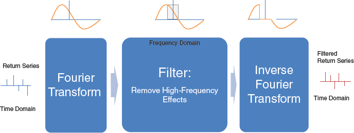
One of the main benefits of converting signals into the frequency domain is that it is relatively easy to filter out different frequencies from a signal. Once the frequency domain signal is filtered it can then be converted back into a time series via the Inverse Fourier Transform. The result is a time signal with high-frequency effects removed from the series. To demonstrate this approach, Figure 14.13 presents a flow chart for the filtering process to remove high-frequency effects. In practical terms, once the high-frequency doubling down effects are removed, it is possible to see how much of the performance in terms of Sharpe ratios was attributed to these accelerating betting schemes.
FIGURE 14.13 A schematic for the process of filtering out high-frequency effects in return series. The inputs are return series in the time domain. Outputs are filtered return series in the time domain. Filtering occurs in the frequency domain.
To make this example even more concrete, the returns of six trend following managers (CTA1 to CTA6) and one trend following program (with and without Martingale betting) can be examined.9 For CTA managers, their performance is converted into the frequency domain and subsequently filtered to remove high-frequency effects. An inverse Fourier transform is then applied to the remaining frequency series to convert it back into a time series. Table 14.4 lists the performance measures for the original Sharpe ratio and postfiltering Sharpe ratios. Graphically, Figure 14.14 plots the original Sharpe ratio and the postfiltering Sharpe ratio without high-frequency effects. Filtering out high-frequency effects reduces the performance for all CTA managers except CTA4. It is important to note that certain managers exhibit more high-frequency effects in their returns than others. For a specific example, CTA2’s performance is cut by more than half when high-frequency effects are removed. This indicates that CTA2 is more likely to use dynamic leveraging in their position taking. More specifically, the Sharpe ratio reduces from 2.01 to 0.94 when high-frequency effects are removed. On the other hand, CTA1 and CTA5 are only mildly affected by removing high-frequency effects. This suggests that these two managers do not accelerate or decelerate positions similar to dynamic leveraging. This point is also true for a trend following system when compared with a trend following system with limited Martingale betting. High-frequency effects explain 0.46 of the performance of trend following with limited Martingale betting and only 0.03 of the performance for a standard trend following program. The difference in Sharpe ratios demonstrates how Fourier transform can be used to analyze the performance impact of dynamic leveraging. This approach is a tool that reveals potential hidden leverage risk due to dynamic leveraging. The Sharpe ratio provides a risk-adjusted performance measure. Despite this risk adjustment, the impact of dynamic leveraging is not always measurable in Sharpe ratios. The use of Fourier transforms allows for the removal of dynamic leveraging effects from return series providing insights into position taking for CTA managers.
TABLE 14.4 The original two-year Sharpe ratio and the two-year Sharpe ratio after removing the dominant high-frequency components for six managers (CTA1 to CTA2) and two trend following systems (TF and TF with limited Martingale betting).
Original Series |
Removing High Frequencies |
|
| CTA1 | 1.05 |
0.84 |
| CTA2 | 2.01 |
0.94 |
| CTA3 | 2.31 |
1.49 |
| CTA4 | 0.64 |
0.69 |
| CTA5 | 2.51 |
2.32 |
| CTA6 | 0.17 |
–0.65 |
| TF | 0.56 |
0.53 |
| TF with Martingale Betting | 1.34 |
0.88 |
FIGURE 14.14 Two-year Sharpe ratios for six trend following CTAs and a representative trend following program with and without limited Martingale betting. Sharpe ratios are calculated with and without filtering out high-frequency effects via Fourier Transform.

■ Summary
This chapter presents three advanced topics from an investor perspective. First, the impact of equity markets on crisis alpha is discussed. A closer analysis of crisis alpha and equity bias demonstrates that equity markets are often the instigator for crisis but not the main driver of performance. Despite this fact, when equity positions are long biased this may improve performance from the manager perspective. From the investor perspective, a long equity bias may increase performance for a manager on a stand-alone basis but in a global perspective this shift comes at the cost of crisis alpha, reducing some of the diversifying properties of the strategy.
Second, the chapter turned to mark-to-market in managed futures. Due to the standardization of mark-to-market in managed futures, high correlations are representative of actual correlations between strategies. In contrast, for strategies outside of managed futures, the lack of standardized mark-to-market mechanisms has the ability to understate correlations between managers overstating the diversification properties of many dynamic hedge fund strategies.
Finally, this chapter turned to cyclicality in volatility for trend following. Even in comparison with equity markets, standard trend following systems exhibit low-frequency cyclicality in volatility. The use of the Fourier transform as a tool to examine the spectral components in trading series is discussed. The discussion of dynamic leveraging as a hidden risk in Sharpe ratios was also reexamined. Using filtering techniques, return series for managers can be filtered for the impact of dynamic leveraging and its corresponding impact on Sharpe ratios. An analysis of several managers demonstrated the heterogeneity across individual managers. In addition, the comparison of trend following systems with and without limited Martingale betting demonstrated the ability of spectral analysis and filtering to capture hidden risks in dynamic leveraging.
■ Further Readings and References
Arakelyan, A., and P. Serrano. “Liquidity in Credit Default Swap Markets.” Mimeo, University CEU Cardenal Herrera, Spain, 2012.
Brunnermeier, M. K., and L. H. Pedersen. “Market Liquidity and Funding Liquidity.” Review of Financial Studies 22, no. 6 (2009): 2201–2238.
Getmansky, M., A. Lo, and I. Makarov. “An Econometric Model of Serial Correlation and Illiquidity in Hedge Fund Returns.” Journal of Financial Economics 74, no. 3 (2004): 529–609.
Greyserman, A. “The Impact of Mark-to-Market on Return Correlations,” ISAM white paper, 2013.
Greyserman, A. “Trend Following in Equity Markets: The Cost of Crisis Alpha.” ISAM white paper, 2012.
Monoyios, M., and L. Sarno. “Mean Reversion in Stock Index Futures Markets: A Nonlinear Analysis.” Journal of Futures Markets 22, no. 4 (2002).
Smith, S. “The Scientist and Engineer’s Guide to Digital Signal Processing.” California Technical Pub., 1997.
Vayanos, D. “Flight to Quality, Flight to Liquidity, and the Pricing of Risk.” NBER Working Paper, 2004.
1 The representative trend following system is a diversified system with equal dollar risk allocation.
2 For the analysis in this section, the equity sector includes two North American markets, four European markets, and three Asian markets.
3 The other scenario for the MDI being larger than 0.1 is when sMDI is lower than –0.1, which counts approximately one-third of the cases.
4 For each investment prior to combining them into a single portfolio, monthly volatility is normalized to 5 percent.
5 Instead of examining long-only positions in the equity sector, again for realistic purposes, a bias of 5:1 for long positions versus short positions is applied.
6 The Fourier transform is a commonly used signal processing tool, converting a signal from the time domain to the frequency domain. For technical details see Smith (1997).
7 In this analysis, all time series are normalized to the same volatility.
8 This concept was introduced and discussed in Chapter 5.
9 The Fourier transform and inverse Fourier transform are performed for the absolute value of returns. After filtering and applying the inverse Fourier transform, the recovered returns are assumed to have the same sign as the original returns. For tractability, extreme outliers in the power spectral density are removed before applying the inverse Fourier transform.