
Few systems achieve scalability these days, because scalability tests are run so infrequently. This chapter shows how to run a scalability test that is so quick-and-easy, you can run it every day of the week, providing much needed guidance to finally steer your SUT toward scalability.
The objectives of this chapter are:
- Learn a formula to determine exactly how many threads or load to apply so you can easily see how close your system is to scaling.
- Learn how to recognize when test data shows you have reproduced a performance problem that is an impediment to scalability.
Trying to fix a defect that you can’t reproduce is daunting, and performance defects are no exception. This chapter walks you through a methodical approach
to reproducing defects that keep your system from scaling. Chapter 8 is where we start using the P.A.t.h. Checklist to diagnose and fix the problems.
The Scalability Yardstick is a variant of the good old incremental load plan, often lost in the annals of performance best practices. This variation is built to show us exactly how much load to apply and how to recognize when we have reproduced a problem, an impediment to scalability.
Scalability is a system’s ability to increase throughput as more hardware resources are added. This definition is accurate and concise, but it is also painfully unhelpful, especially if, like most technicians, you are looking for concrete direction on how to make your system scale.
To fill this void and provide a little direction, I use the following load test
that I call the Scalability Yardstick:
- 1.Run an incremental load test with four equal steps of load, the first of which pushes the app server CPU to about 25%.
- 2.When this test produces four squared, chiseled steps of throughput, the last of which pushes the CPU to 100%, the SUT is scalable.
Let’s start by seeing how to use the load generator to create a load plan for the Yardstick, and then we will talk about how scalability actually works. It takes a little bit to explain this approach, but it becomes second nature after you do it a few times.
Creating a Scalability Yardstick Load Plan
The Scalability Yardstick says that your first step of load needs to push the SUT to consume about 25% of the CPU. How many threads of load will it take to reach 25%? You need to run a quick test to find out. This essentially calibrates the Yardstick to the SUT and this environment.
The JMeter test plan
shown in Figure 6-1 asks the question, “At which of these 10 steps will the SUT CPU consumption reach 25%?”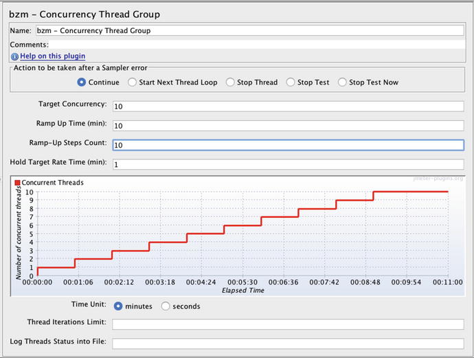
Figure 6-1.
JMeter load plan
used to see how many threads of load it takes to push the application server CPU to 25%
Here are some brief instructions for doing this:
- 1.Install JMeter from jmeter.apache.org.
- 2.Install the Concurrency Thread Group using one of these two options:
- 1.Install the Plugin Manager into JMeter by downloading a jar from here:https://jmeter-plugins.org/install/Install/ into the JMETER/home/ext directory. Restart JMeter and then select Custom Thread Groups from the Options / Plugins menu.
- 2.Download the zip file directly from here:https://jmeter-plugins.org/wiki/ConcurrencyThreadGroup/ …and unzip the contents into JMETER_HOME/lib and lib/ext folders, as they are in the zip file.
- 1.
- 3.Restart JMeter.
- 4.Add the Concurrency Thread Group using the menu options in Figure 6-2.
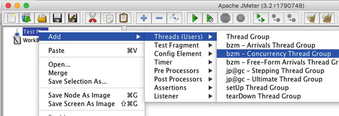 Figure 6-2.Adding the Concurrency Thread Group to a new JMeter load plan.
 - 5.Dial in the 10-10-10-1 options in Figure 6-1.
Figure 6-3 shows the results of this short little calibration test, or at least the very first part of it. By the time the test reached just the second of 10 steps, I had seen enough, so I stopped it.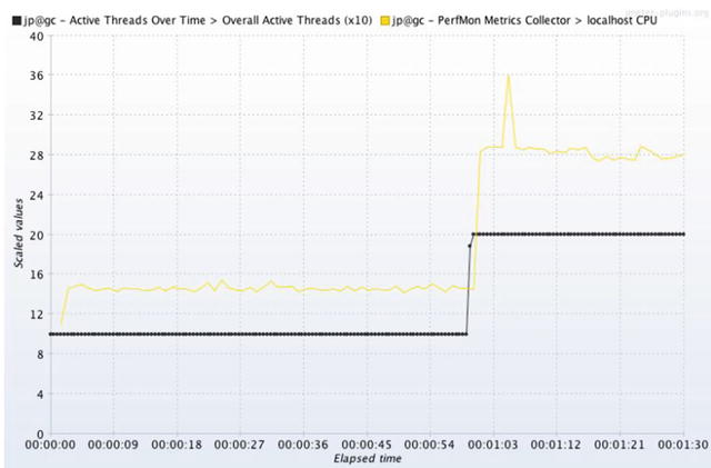
Figure 6-3.
Discovering how many threads
it takes to push the CPU to 25%. This graph with two different metrics (CPU and active threads) was made possible by Composite Graph and PerfMon, both from jmeter-plugins.org. Learn how to use them in Chapter 7 on JMeter.
The load plan in Figure 6-1 shows that each step of load should have lasted about 60 seconds, and it did. We know this because the black line (below Active Threads Over Time
) travels at a Y axis value of 10 for 60 seconds, then at 20 for the rest of the test. The autoscaling on this graph is a big confusing. The (x10) that is displayed in the legend means the 10 and the 20 are magnified by 10 on the graph, and are actual values of 1 and 2 instead of 10 and 20.
The yellow line in Figure 6-3 shows that the first thread of load pushed the CPU to about 15% and the second thread (at the 60 second mark) pushed the CPU to about 28%. The whole purpose of the test was to push the SUT to at least 25%, so I stopped the load generator after the step that first hit 25%. The calibration is complete.
The Yardstick says we need “four equal steps of load, the first of which pushes the CPU to about 25%.” Since two threads pushed the SUT to about 25% CPU, 2 is the size of each of the four equal steps in the Yardstick. We now know enough to create our Yardstick load plan.
Interpreting Results
The calibration test is complete, and you know about how many threads of load it takes to push the SUT to about 25% CPU consumption. I took the result of 2 from the Calibration Test and put it into my load plan to create a Scalability Yardstick test with steps of 2-4-6-8. Every minute, two threads of load are added; for the last minute of the 4-minute test, eight threads are running. Staying at a single level of load for 1 minute works when a single iteration of your load script lasts, say, less than 10 seconds with zero think time. This is a very rough guideline to make sure your script repeats at least several times (six in this case) for each step of load.
Figure 6-4 shows the results of the test. This part takes a little thinking, so get ready for this: the x100 in the legend (top of screenshot) mean the black line values of 200, 400, 600 and 800 really mean 2, 4, 6, and 8 load generator threads. The jmeter-plugins.org auto-scale feature caused this. Read here for more details: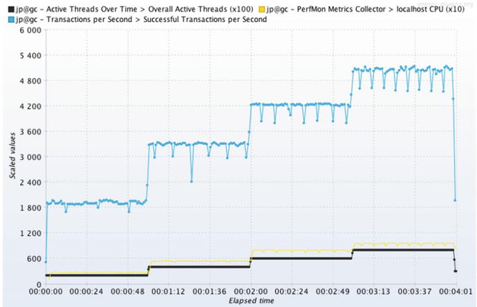
Figure 6-4.
The blue line shows squared, chiseled steps of throughput created by the Scalability Yardstick, meaning that this system will scale. To produce this graph, the Throughput metric was added to the same graph component used in Figure 6-3.
The Scalability Yardstick aims to find the SUT’s throughput at 25%, 50%, 75% and 100% CPU consumption, and Figure 6-4 shows that. The blue line shows these four throughput landmarks are (roughly) 1800, 3300, 4200 and 5100 requests per second. Because each of the four steps generates a nicely squared chunk of throughput, this particular SUT is very well tuned.
By contrast, Figure 6-5 shows an SUT with a performance defect
. See how the squared, chiseled steps of load have been replaced by limp, faltering throughput?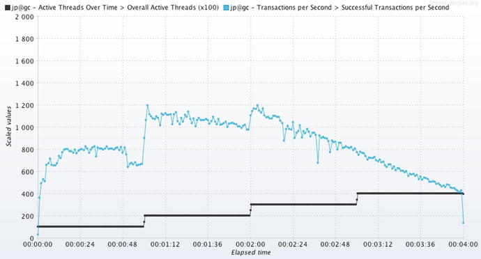
Figure 6-5.
The same graph configuration
of Figure 6-4 was used here, but I induced a performance defect (high GC times I think) to make the squared, chiseled steps go away. This is how systems perform when they don’t scale.
To those who are hesitant to push the CPU to 100%, how else will we discover whether the system is capable of using an additional CPU, should one become available? We know that pushing the CPU to 100% is not going to hurt the machine, because anti-virus software has been doing that to desktop workstation CPUs for a decade.
Here are a few quotes from other Java performance
authors that show that this approach is on the right track, especially the part about pushing to 100% CPU:
“The goal is to usually keep the processors fully utilized.”Java Concurrency in Practice, Brian Goetz, et al. (Addison-Wesley, 2006) p. 240“For a well-behaved system, the throughput initially increases as the number of concurrent users increases while the response times of the requests stay relatively flat.”Java Performance, Charlie Hunt, Binu John (Addison-Wesley, 2011), p. 369
Driven by the black line in Figure 6-4, each of the four steps in the Yardstick acts as a request for the SUT
to leap. The four steps in the blue throughput line shows that the SUT
responded with a leap for each load step. Take the utmost care in noticing that a nice square, step/leap of additional CPU consumption (yellow) was required at each step. When the load generator said to leap, the SUT leapt, and only a well-tuned and scalable SUT will leap like this.
Of the four CPU landmarks in the Scalability Yardstick, we care the most about the 100% landmark. We ultimately want to know whether the SUT can utilize 100% of this CPU and 100% of all the subsequently added CPUs to produce more and more throughput leaps when the load generator applies additional steps of throughput. This is scalability.
Let’s walk through a quick example of how to use these numbers. Let’s say that our client is upgrading from someone else’s system to our system. Data from peak hours of their previous system shows the client needs to reach 6,000 requests per second (RPS).
Let’s use the graph from the Scalability Yardstick test in Figure 6-4. It shows that we are in trouble—the 5,100 RPS in the graph falls a bit short because we ran out of CPU before getting to the client’s 6,000 RPS target. What is to be done? We need to do the impossible—to push from 100% to 101% CPU consumption and beyond. It is as if someone wanted the volume nob on their car radio to go past the max of 10 and on to 11.
To get to the 6,000 RPS, we have to add more machines to share the burden (to form a cluster), using a load balancer to distribute the load between the machines. Alternatively, we can add additional CPUs to the original machine. This is the classic and powerful concept of scalability.
When an application on a single machine can incrementally turn every bit of the CPU into a decent amount of throughput, it is straightforward to see how it would also be capable of using additional CPUs, once they were made available.
Figure 6-5 depicts the system without the squared, chiseled steps—it’s the one that did not scale. Without more tuning, it has no hope of scaling, because the throughput won’t approach 6000, no matter how many threads of load are applied.
If adding additional users won’t buy extra throughput, the system will not scale. That is the lesson here.
Imperfect and Essential
I will never forget this painful story about tuning. We were beaten down and exhausted after 12 weeks of gruelling, long hours trying to reach an unprecedented amount of throughput for an especially demanding client. The crowded and stale conference room was so quiet, you might not have known we were actually celebrating, but we were—just too exhausted to get excited. The system finally scaled, or at least we thought it did. Doubling the hardware had doubled the throughput—that much was good. Tripling the hardware tripled the throughput, but that was the end of the scalability, and after that the quiet room got busy again. No one predicted this problem because the problem was not predictable.
The Scalability Yardstick test, like all forecasting tools, is imperfect; it cannot predict what has not been tested, just as in this little (and mostly true) anecdote. But even though scalability tests are imperfect, they are still essential. The Yardstick measures a key facet of all scalable systems: the ability to produce even steps of throughput at all levels of CPU consumption
. Without such a tool, we stumble blindly through the development SDLC phase and beyond, knowing nothing of our progress towards the very goal we seek: scalability.
Back in the crowded conference room, there was progress. A concurrency cap, configured on the load balancer, had kept additional nodes from producing any more throughput. After fixing the configuration, adding a fourth node in our system quadrupled the throughput, pushing us past our difficult goal, and demonstrating great scalability.
Reproducing Bad Performance
As mentioned, the 100% CPU landmark is important for demonstrating scalability. The other three landmarks (25%, 50%, 75%) serve as little breakpoint tests for all those applications that do not perform as well as the SUT in Figure 6-4—which means most applications. The CPU landmarks show exactly how much load you need to apply to reproduce a performance problem. For example, let us say that you have nice chiseled and squared steps at the first two load increments (25% and 50% CPU), but throughput will not climb and the CPU will only push to, say, 55% in the third load increment. Bingo. You have reproduced the problem, which is the first part of “seeing” the problem. The second and last part of “seeing” the problem is to look at the right performance data using the right monitoring tools, as described in P.A.t.h. chapters, starting in Chapter 8.
When a seemingly formidable opponent is taken down by a lesser challenger, headlines are quick to hail the underdog and disgrace the dethroned champion. Likewise, if a seemingly robust SUT exhibits a monumental performance problem with very few threads of load, this is a critical problem, indeed. The smaller the amount of load required to reproduce a performance defect, the more critical the problem. As such, reproducing a problem at 25% CPU shows a much more critical problem than that same issue produced at a higher CPU percentage. Don’t forget that the priority and/or criticality that you designate for an issue in a defect tracking system should somehow reflect this. Additionally, an unnecessarily high amount of load often introduces others issues (like the concurrency cap issues discussed in Chapter 5 on invalid load tests), that complicate an already difficult troubleshooting process. The lesson here is to apply only as much load as it takes to reproduce the problem—any more load than that unnecessarily complicates matters.
Once the Scalability Yardstick establishes the smallest amount of throughput required to transition from chiseled steps into erratic chaos and thus demonstrate a performance problem, it is helpful to switch from the Yardstick load plan to a steady-state load plan. You can then change the load plan to extend the duration of the test—the goal is to provide ample time to review the P.A.t.h. Checklist and start capturing data from the monitoring and tracing tools.
Once the problem has been identified and a fix deployed, a rerun of the steady-state test provides a great before-after comparison and a compelling story for your team. If the system change brings us closer to our performance goals (higher throughput and/or lower response time and/or lower CPU consumption), then the change is kept and the cycle begins again by rerunning the Yardstick to see where the next problem lies. Remember that the fix has changed the performance landscape and you will likely need to recalibrate the Yardstick by rerunning the Yardstick Calibration test.
We use the Scalability Yardstick
for two purposes: measure the best throughput and reproduce performance defects. When the detect-reproduce-fix cycle all happens on a single machine/environment, the single-threaded workflow drags to a slow crawl: developers are forced to stand in line to run another test on the “golden” environment to get feedback on proposed code fixes. Comparing the performance of multiple code options is thus rendered infeasible, because access to the busy golden environment is in high demand. To get around this, the best performance engineers are skilled at enabling developers to work independently, to reproduce performance defects themselves, perhaps on their own desktops, and perhaps even comparing the performance of multiple design approaches. This is yet another benefit of the Modest Tuning Environment discussed back in Chapter 2.
Good and Bad CPU Consumption
Not all high CPU consumption
is bad, especially when scalability is important. In fact, if building scalable systems is part of our goal, then we should actively drive systems to make leaps in throughput, while using all 100% of the CPU, at least in test environments. Of course, CPU that does not contribute to throughput is bad. For example, consider the case when the CPU hits 100% during application server start up when no load is applied. This is bad CPU.
One way to look at bad performance is that it is caused by either too little or too much CPU consumption. The first kind, “too little CPU,” behaves like this: no matter how many threads of load are applied, the SUT throughput will not climb much, even though there is plenty of available CPU. The SUT acts as if an unimaginably heavy blanket, one that is many times heavier than the lead apron you wear to protect your body during a chest x-ray, has been cast on top of the frail throughput and CPU lines, holding them down, keeping them from making the responsive throughput leaps found in scalable systems.
As such, when that heavy blanket camps out on top of your SUT, using faster CPUs will provide only marginal benefits. Adding more of the same kind of CPU will just damage your pocketbook.
I will defend to the death the reasoning behind driving CPU consumption up to 100%, especially when throughput is bursting through the ceiling.
Why? If it is not proof of scalability, it is certainly a required attribute thereof. Flirting with 100% CPU like this is understandable, but there is no sense in applying more load if the CPU is already at 100%. As part of a negative test, this might be helpful, but it is a dead end when you are looking for more throughput.
Even when faced with really low throughput, technicians sometimes boast about their SUT’s low CPU consumption. It takes work to help them figure out that, in this light, low CPU
consumption is bad and not good. On the other hand, low CPU consumption is good when you are comparing two tests whose performance is alike in every way (especially throughput), except that CPU is lower on one.
With the second kind of poor performance, “too much CPU,” the SUT burns through so much CPU that you would need an entire farm of busily grazing CPUs to generate enough throughput to meet requirements, when a better-tuned SUT would just require a few CPUs, slowly chewing cud. This is why its helpful to introduce a performance requirement that caps the amount of money spent on hardware.
“Too much CPU” should guide us to optimize code that is both unnecessary and CPU hungry. The tools to point out which code is CPU hungry are discussed in the P.A.t.h. Checklist for threads, Chapter 11. And whether code is unnecessary is of course subjective, but there are some great, concrete examples of unnecessary code in that same Chapter 11. “Too little CPU” indicates that contention or I/O or other response time issues are holding back the system from generating enough throughput. Guidance for addressing these problems is scattered throughout four chapters covering the P.A.t.h. Checklist, starting in Chapter 8.
Chapter 2 on Modest Tuning Environments encourages us to run more fix-test cycles every day, with the expectation that improvements will ensue. That means the performance landscape is fluid and needs to be re-evaluated between optimizations. Just an optimization or two can easily turn a “too much CPU” system into a “too little CPU” system. For instance, suppose a number of systems with complex security requirements query a database for hundreds of permissions for each user, and let’s further say that a review of the entire P.A.t.h. Checklist shows this is the worst problem in the system. Once you add caching to this CPU-intensive approach, you will discover the next worst problem in the system, which very well might be contention (discussed in Chapter 11), which leaves us with a “too little CPU” system.
Be careful how others perceive your attempts to push CPU to 100%, as with the Scalability Yardstick. Rightfully, data center owners require plenty of assurances that production applications will meet throughput requirements while consuming modest portions of the allotted CPU. Ask them how much consumption they feel comfortable with. The risk of running out of CPU is too great, especially when human error and other operational blunders can unexpectedly drive up CPU consumption. Sometimes business processes get inadvertently left out of the tuning process altogether, and their CPU-hungry nature ambushes you in production. Sneak attack.
Don’t Forget
I am not a carpenter, but even I know that you measure twice and cut once to fashion a board to the right dimensions. With software, we generally measure scalability zero times before checking into source code control. Zero times.
Once the clay has been baked, the sculptor is done. If you wanted that malformed mug to instead be a fancified chalice, you are out of luck. If that clay bust of your benefactor looks more like a sci-fi monster with three noses, sorry. The development process is our golden window of opportunity to sculpt and reshape the code, and we currently let that opportunity sail right on by without ever checking in on our progress towards our scalability goal. Does it have the right number of noses? Does it still look like a monster? Why do we never ask these obvious questions until it is way too late?
The Scalability Yardstick is quick and easy to use; it enables us to measure performance progress frequently during the development process, while our window of opportunity is open to set things right, before the clay is baked.
When our system scales, the load generator pushes the SUT to produce clean, chiseled leaps/steps of throughput. Instead of the squared and chiseled throughput (and other) metrics, poor performing SUTs have jagged, impotent and weighted down throughput because the code is littered with contention, as shown by the jagged variability in individual metrics.
I have mentioned that applying an unrealistically large amount of load is a common mistake, perhaps even an anti-pattern. 3t0tt helps address this problem—it is a nice, safe way to keep pretentious performance engineers like myself from lecturing about unrealistically high load. 3t0tt is a fantastic starting point, but it doesn’t tell you whether your system scales—you need the Scalability Yardstick for that.
What’s Next
This chapter focused on the interplay between throughput, CPU and the amount of load applied. Seeing these three metrics on the same graph was helpful to running the Scalability Yardstick test. In Chapter 7, coming up next, we will see how to put all these metrics on the exact same JMeter graph. Chapter 7 is a deep dive into the JMeter basics that deserve being repeated, and into important JMeter features and foibles that seem underdocumented.