
![]()
Working with Data Files
Before you can begin any statistical analysis, you will need to learn to work with external data files so that you can import your data. R is able to read the comma-separated values (CSV), tab-delimited, and data interchange format (DIF) file formats, which are some of the standard file formats commonly used to transfer data between statistical and database packages. With the help of an add-on package called foreign, it is possible to import a wider range of file types.
Whether you have personally recorded your data on paper or in a spreadsheet, or received a data file from someone else, this chapter will explain how to get your data into R.
You will learn how to:
- enter your data by typing the values in directly
- import plain text files, including the CSV, tab-delimited, and DIF file formats
- import Excelâ files by first converting them to the CSV format
- import a dataset stored in a file type specific to another software package such as an SPSS or Stata data file
- work with relative file paths
- export a dataset to a CSV or tab-delimited file
Entering Data Directly
If you have a small dataset that is not already recorded in electronic form, you may want to input your data into R directly.
Consider the dataset shown in Table 2-1, which gives some data for four U.K. supermarkets chains. It is representative of a typical dataset in which the columns represent variables and each row holds one observation.
Table 2-1. Data for the U.K.’s Four Largest Supermarket Chains (2011); see Appendix C for more details
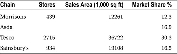
To enter a dataset into R, the first step is to create a vector of data values for each variable using the c function, as explained under “Vectors” in Chapter 1. So, for the supermarkets data, input the four variables:
> Chain<-c("Morrisons", "Asda", "Tesco", "Sainsburys")
> Stores<-c(439, NA, 2715, 934)
> Sales.Area<-c(12261, NA, 36722, 19108)
> Market.Share<-c(12.3, 16.9, 30.3, 16.5)
The vectors should all have the same length, meaning that they should contain the same number of values. Where a data value is missing, enter the characters NA in its place. Remember to put quotation marks around non-numeric values, as shown for the Chain variable.
Once you have created vectors for each of the variables, use the data.frame function to combine them to form a data frame:
> supermarkets<-data.frame(Chain, Stores, Sales.Area, Market.Share)
You can check the dataset has been entered correctly by entering its name:
> supermarkets
        Chain   Stores   Sales.Area   Market.Share
1   Morrisons      439        12261           12.3
2        Asda       NA           NA           16.9
3       Tesco     2715        36722           30.3
4  Sainsburys      934        19108           16.5
After you have created the data frame, the individual vectors still exist in the workspace as separate objects from the data frame. To avoid any confusion, you can delete them with the rm function:
> rm(Chain, Stores, Sales.Area, Market.Share)
Importing Plain Text Files
The simplest way to transfer data to R is in a plain text file, sometimes called a flat text file. These are files that consist of plain text with no additional formatting and can be read by plain text editors such as Microsoft Notepad, TextEdit (for Mac users), or gedit (for Linux users). There are several standard formats for storing spreadsheet data in text files, which use symbols to indicate the layout of the data. These include:
- Comma-separated values or comma-delimited (.csv) files
- Tab-delimited (.txt) files
- Data interchange format (.dif) files
These file formats are useful because they can be read by all of the popular statistical and database software packages, allowing easy transfer of datasets between them.
The following subsections explain how you can import datasets from these standard file formats into R.
Comma-separated values (CSV) files are the most popular way of storing spreadsheet data in a plain text file. In a CSV file, the data values are arranged with one observation per line and commas are used to separate data value within each line (hence the name). Sometimes semicolons are used instead of commas, such as when there are commas within the data itself. The tab-delimited file format is very similar to the CSV format except that the data values are separated with horizontal tabs instead of commas. Figures 2-1 and 2-2 show how the supermarkets data looks in the CSV and tab-delimited formats. These files are available with the downloads for the book (www.apress.com/9781484201404).
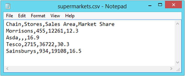
Figure 2-1. The supermarkets dataset saved in the CSV file format
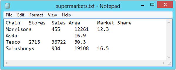
Figure 2-2. The supermarkets dataset saved in the tab-delimited file format
You can import a CSV file with the read.csv function:
>dataset1<-read.csv("C:/folder/filename.csv")
This command imports data from the file location C:/folder/filename.csv and saves it to a data frame called dataset1.
Remember that when choosing a dataset name, the usual object naming rules apply (see the “Objects” section in Chapter 1). It is a good idea to choose a short but meaningful name that describes the data in the file.
The file path C:/folder/filename.csv is the location of the CSV file on your hard drive, network drive, or storage device. Notice that you must use forward slashes to indicate directories instead of the back slashes used by Windows, and that you must enclose the file path between quotation marks. For Mac and Linux users, the file path will begin with a forward slash, for example, /Users/username/folder/filename.csv.
If the dataset has been successfully imported, there is no output and R displays the command prompt once it has finished importing the file. Otherwise, you will see an error message explaining why the import failed. Assuming there are no issues, your data will be stored in the data frame named dataset1. You can view and check the data by typing the dataset name at the command prompt, or by opening it with the data editor.
For importing tab-delimited files, there is a similar function called read.delim:
>dataset1<-read.delim("C:/folder/filename.txt")
When you use the read.csv or read.delim functions to import a file, R assumes that the entries in the first line of the file are the variable names for the dataset. Sometimes R will adjust the variable names so that they follow the naming rules (see the “Objects” section in Chapter 1) and are unique within the dataset.
If your file does not contain any variable names, set the header argument to F (for false), as shown here. This prevents R from using the first line of your data as the variable names:
>dataset1<-read.csv("C:/folder/filename.csv", header=F)
When you set the header argument to F, R assigns generic variable names of V1, V2, and so on. Alternatively, you can supply your own names with the col.names argument:
> dataset1<-read.csv("C:/folder/filename.csv", header=F, col.names=c("Name1", "Name2", "Name3"))
When using the col.names argument, make sure that you give the same number of names as there are variables in the file. Otherwise, you will either see an error message or find that some of the variables are left unnamed.
In a CSV or tab-delimited file, missing data is usually represented by an empty field. However, some files may use a symbol or character such as a decimal point, the number 9999, or the word NULL as a place holder. If so, use the na.strings argument to tell R which characters to interpret as missing data:
>dataset1<-read.csv("C:/folder/filename.csv", na.strings=".")
Note that R automatically interprets the letters NA as indicating missing data. Blank spaces found in numeric variables (but not character variables) are also recognized as missing data.
In some parts of the world, a comma is used instead of a dot to denote the decimal point in numbers. Figure 2-3 shows a tab-delimited file with numbers in this format. R has two special functions for dealing with data in this form, called read.csv2 and read.delim2, which you can use in place of the read.csv and read.delim functions.
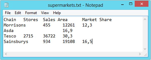
Figure 2-3. The supermarkets dataset saved in the tab-delimited file format, with commas used to represent the decimal point
To import a data interchange format (DIF) file with the .dif file name extension, use the read.DIF function:
>dataset1<-read.DIF("C:/folder/filename.dif")
By default, the read.DIF function assumes that there are no variable names in the file (unlike the read.csv and read.delim functions). If the file does contain variable names, set the header argument to T (for true), as shown below. Otherwise, R will treat the variable names as part of the data values:
>dataset1<-read.DIF("C:/folder/filename.dif", header=T)
As when importing CSV and tab-delimited files, you can use the na.strings argument to tell R about any values that it should interpret as missing data:
>dataset1<-read.DIF("C:/folder/filename.dif", na.string="NULL")
Note that if you are importing a DIF file that was created by Microsoft Excel, you may see the error message 'More rows than specified in header'; maybe use 'transpose=TRUE' when you try to import the file. This error message appears because some versions of Microsoft Excel use a modified version of the DIF file format instead of the standard one. You can resolve the problem by setting the transpose argument to T:
>dataset1<-read.DIF("C:/folder/filename.dif", transpose=T)
As well as all of the functions available for importing specific file formats, R also has a generic function for importing data from plain text files called read.table. It allows you to import any plain text file in which the data is arranged with one observation per line.
Consider the file shown in Figure 2-4, which has data arranged with one observation per line and data values separated by the forward slash symbol (/).
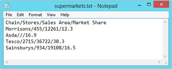
Figure 2-4. The supermarkets data in a nonstandard file type
You could import the file with this command:
>dataset1<-read.table("C:/folder/supermarkets.txt", sep="/", header=T)
By default, the read.table function assumes that there are no variable names in the first row of the file (unlike the read.csv and read.delim functions). If the file has variable names in the first row (as in this example), set the header argument to T.
As with the other import functions, you can use the na.strings argument to tell R of any values to interpret as missing data:
dataset1<-read.table("C:/folder/filename.txt", sep="/", header=T, na.strings="NULL")
The simplest way to import a Microsoft Excel file is to save your Excel file as a CSV file, which you can then import, as explained earlier in this chapter under “CSV and Tab-Delimited Files.”
First open your file in Excel and ensure that the data is arranged correctly within the spreadsheet, with one variable per column and one observation per row. If the dataset includes variable names, then these should be placed in the first row of the spreadsheet. Otherwise, the data values should begin on the first row. Figure 2-5 shows how the supermarkets data looks when correctly arranged in an Excel file.
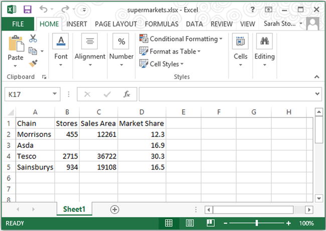
Figure 2-5. The correct way to arrange a dataset in an Excel spreadsheet, to facilitate easy conversion to the CSV file format
To ensure a smooth file conversion, check the following:
- There are no empty cells above or to the left of the data grid
- There are no merged cells
- There is no more than one row of column headers
- There is no formatting such as bold, italic or colored text, cell borders or background colors
- Where data values are missing, the cell is left empty
- There are no commas in large numbers (e.g., 1324157 is acceptable but 1,324,157 is not)
- If exponential (scientific) notation is used, the format is correct (e.g., 0.00312 can be expressed as 3.12e-3 or 3.12E-3)
- There are no currency, unit, or percent symbols in numeric variables (symbols in categorical variables or in the variable names are fine)
- The minus sign is used to indicate negative numbers (e.g., -5) and not brackets (parentheses) or red text
- The workbook has only one worksheet
When the data is prepared, save the spreadsheet as a CSV file by selecting Save As from the File menu. When the Save As dialog box appears, select the .csv file type from the Save As Type field, as shown in Figure 2-6. Then save the file as usual. Excel will give you a warning that all formatting will be lost, which you can accept.

Figure 2-6. Saving an Excel file as a CSV file
The CSV file is now ready for you to import with the read.csv function, as explained previously in this chapter (see “CSV and Tab-Delimited Files”).
If you do not have access to Excel, you can use an add-on package such as xlsx or xlsReadWrite to import Excel files directly. See Appendix B for more details on using add-on packages.
Importing Files from Other Software
Sometimes you may need to import a dataset that is saved in a file format specific to another statistical package, such as an SPSS or Stata data file.
If you have access to the software, the simplest solution is to open the file using the software and convert the file to the CSV file format using the Save As or Export option, which is usually found in the File menu. Once the file is in CSV format, you can import it with the read.csv function (see “CSV and Tab-Delimited Files” earlier in this chapter).
If you are not able to convert the file, then you can use an add-on package called foreign, which allows you to directly import data from files types produced by some of the popular statistical software packages.
Add-on packages are covered in greater detail in Appendix A. For now, you just need to know that an add-on package contains additional functions that are not part of the standard R installation. To use the functions within the foreign package, you must first load the package.
To load the foreign package, select Load Package from the Packages menu. When the list of packages appears, select “foreign” and press OK. Once the package has loaded, all of the functions within it will be available for you to use for the duration of the session.
Table 2-2 lists some of the functions available for importing foreign file types.
Table 2-2. Some of the Functions Available in the Foreign Add-on Package
File type |
Extension |
Function |
|---|---|---|
Database format file |
.dbf |
read.dbf |
Stata versions 5 to 12 data file |
.dta |
read.dta |
Minitab portable worksheet file |
.mtp |
read.mtp |
SPSS data file |
.sav |
read.spss |
SAS transfer format |
.xport |
read.xport |
Epi Info data file |
.rec |
read.epiinfo |
Octave text data file |
.txt |
read.octave |
Attribute-relation file |
.arff |
read.arff |
Systat file |
.sys, .syd |
read.systat |
For example, to import a Stata data file, use the command:
>dataset1<-read.dta("C:/folder/filename.dta")
You may need to use additional arguments to ensure the file is imported correctly. For further information on using the functions in the foreign package, use the help function or refer to the package documentation available from the R project website at cran.r-project.org/web/packages/foreign/foreign.pdf.
So far, we have only used absolute file paths to describe the location of a data file. An absolute file path gives the full address of the file, which in the Windows environment begins with a drive name such as C:/.
You can also use relative file paths, which describe the location of the file in relation to the working directory. The working directory is the directory in which R is set to look when given relative file paths. This is useful if you need to import or export a large number of files and don't want to type the full file path each time. To see which is the current working directory, use the command:
> getwd()
If you are using a fresh installation of R for Windows, the working directory will be your Documents folder, and R will output something like this:
[1] "C:/Users/Username/Documents"
For Mac and Linux users, the default working directory will be your home directory and will look something like this:
[1] "/Users/Username"
So, to import a CSV file that has the absolute file path:
C:/Users/Username/Documents/Data/filename.csv
you could use the command:
> read.csv("Data/filename.csv")
To change the working directory to wherever you prefer to store your data files, use the setwd function, as shown below. The change is applied for the remainder of the session:
> setwd("C:/folder/subfolder")
R allows you to export datasets from the R workspace to the CSV and tab-delimited file formats.
To export a data frame named dataset to a CSV file, use the write.csv function:
> write.csv(dataset, "filename.csv")
For example, to export the Puromycin dataset to a file named puromycin_data.csv, use the command:
> write.csv(Puromycin, "puromycin_data.csv")
This command creates the file and saves it to your working directory (see the preceding section, “Using Relative File Paths,” for how to find and set the working directory). To save the file somewhere other than in the working directory, enter the full path for the file:
> write.csv(dataset, "C:/folder/filename.csv")
If a file with your chosen name already exists in the specified location, R overwrites the original file without giving a warning. You should check the files in the destination folder beforehand to make sure that you are not overwriting anything important.
The write.table function allows you to export data to a wider range of file formats, including tab-delimited files. Use the sep argument to specify which character should be used to separate the values. To export a dataset to a tab-delimited file, set the sep argument to " " (which denotes the tab symbol):
> write.table(dataset, "filename.txt", sep=" ")
By default, the write.csv and write.table functions create an extra column in the file containing the observation numbers. To prevent this, set the row.names argument to F:
> write.csv(dataset, "filename.csv", row.names=F)
With the write.table function, you can also prevent variable names being placed in the first line of the file with the col.names argument:
> write.table(dataset, "filename.txt", sep=" ", col.names=F)
Summary
You should now be able to get your data into R, whether by entering it directly or by importing it from an external data file. You should also understand how to use relative file paths and be able to export a dataset to an external file.
This table summarizes the most import commands covered in this chapter.
Task |
Command |
|---|---|
Create data frame |
dataset<-data.frame(vector1,vector2,vector3) |
Import CSV file |
dataset<-read.csv("filepath") |
Import tab-delimited file & |
dataset<-read.delim("filepath") |
Import DIF file |
dataset<-read.DIF("filepath") |
Import other text file |
dataset<-read.table("filepath, sep="?") |
Display working directory |
getwd() |
Change working directory |
setwd("C:/folder/subfolder") |
Export dataset to CSV file |
write.csv(dataset, "filename.csv") |
Export dataset to tab-delimited file |
write.table(dataset, "filename.txt",sep=" ") |
Now that you have learned how to get your dataset into R, we can move on to Chapter 3, which explains how to prepare your dataset for analysis.