
![]()
Preparing and Manipulating Your Data
After you have imported your dataset, it is likely that you will need to make some changes before beginning any statistical analysis. You may require some new variables for your analysis, or there may be some irrelevant data that needs to be removed. Additionally, you may want to ensure that variables and categories are correctly named so that they look more presentable on any statistical output that you create. This chapter explains how you can make these types of changes to a dataset.
You will learn how to:
- rename, rearrange, and remove variables
- change the data type of variables
- calculate new variables from old ones
- divide numeric variables into categories
- modify category names for categorical (factor) variables
- manipulate character strings
- work with dates and times
- add or remove observations
- select a subset of data, either by type or as a random sample
- sort the data
More complex changes, such as combining two datasets or changing the structure of the data, are covered in Chapter 4.
This chapter uses the people dataset shown in Figure 3-1 for demonstration purposes. This dataset gives the eye color (brown, blue, or green), height in centimeters, hand span in millimeters, sex (1 for male, 2 for female), and handedness (L for left-handed, R for right-handed) of sixteen people.

Figure 3-1. The people dataset
This chapter also uses the pulserates, fruit, flights, customers, and coffeeshop datasets, which are all available with the downloads for this book (www.apress.com/9781484201404) in CSV format or in an R workspace file. For more information about these datasets, see Appendix C.
Variables
If your dataset has a large number of variables, you can make it more manageable by removing any unnecessary variables and arranging the remaining variables in a meaningful order. You should check that each variable has an appropriate name and an appropriate class for the type of data that it holds, as explained in the following sections.
Rearranging and Removing Variables
You can rearrange or remove the variables in a dataset with the subset function. Use the select argument to choose which variables to keep and in which order. Remove unwanted variables by excluding them from the list.
For example, this command removes the Subject, Height and Handedness variables from the people dataset, and rearranges the remaining variables so that Hand.Span is first, followed by Sex then Eye.Color:
> people1<-subset(people, select=c(Hand.Span, Sex, Eye.Color))
Figure 3-2 shows how the new dataset looks after the changes have been applied.

Figure 3-2. The people1 dataset, created by removing variables from the people dataset with the subset function
Notice that the command creates a new dataset called people1, which is a modified version of the original, and leaves the original dataset unchanged. Alternatively, you can overwrite the original dataset with this modified version:
> people<-subset(people, select=c(Hand.Span, Sex, Eye.Color))
The subset function does more than remove and rearrange variables. You can also use it to select a subset of observations from a dataset, which is explained later in this chapter under “Selecting a subset according to selection criteria”.
Another way of removing variables from a dataset is with bracket notation. This is particularly useful if you have a dataset with a large number of variables and you only want to remove a few. For example, to remove the first, third, and sixth variables from the people dataset, use the command:
> people1<-people[-c(1,3,6)]
Similarly, to retain the second, fourth, and first variables and reorder them, use the command:
> people1<-people[c(2,4,1)]
![]() Note See Chapter 1 under “Data Frames” for more details on using bracket notation.
Note See Chapter 1 under “Data Frames” for more details on using bracket notation.
The names function displays a list of the variable names for a dataset:
> names(people)
[1] "Subject" "Eye.Color" "Height" "Hand.Span" "Sex" "Handedness"
You can also use the names function to rename variables. This command renames the fifth variable in the people dataset:
> names(people)[5]<-"Gender"
Similarly, to rename the second, fourth, and fifth variables:
> names(people)[c(2,4,5)]<-c("Eyes", "Span.mm", "Gender")
Alternatively you can rename all of the variables in the dataset simultaneously:.
> names(people)<-c("Subject", "Eyes", "Height.cm", "Span.mm", "Gender", "Hand")
Make sure that you provide the same number of variable names as there are variables in the dataset.
Each of the variables in a dataset has a class, which describes the type of data the variable contains. You can view the class of a variable with the class function:
> class(dataset$variable)
To check the class of all the variables simultaneously, use the command:
> sapply(dataset, class)
A variable’s class determines how R will treat the variable when you use it in statistical analysis and plots. There are many possible variable classes in R, but only a few that you are likely to use:
numeric variables contain real numbers, meaning positive or negative numbers with or without a decimal point. They can also contain the missing data symbol (NA)
integer variables contain positive or negative numbers without a decimal point. This class behaves in much the same way as the numeric class. An integer variable is automatically converted to a numeric variable if a value with a fractional part is included
factor variables are suitable for categorical data. Factor variables generally have a small number of unique values, known as levels. The actual values can be either numbers or character strings
date & POSIXlt variables contain dates or date-times in a special format, which is convenient to work with
character variables contain character strings. A character string is any combination of unicode characters including letters, numbers, and symbols. This class is suitable for any data that does not belong to one of the other classes, such as reference numbers, labels, and text, giving additional comments or information
When you import a data file using a function such as read.csv, R automatically assigns each variable a class based on its contents. If a variable contains only numbers, R assigns the numeric or integer class. If a variable contains any non-numeric values, it assigns the factor class.
Because R does not know how you intend to use the data contained in each variable, the classes that it assigns to them may not always be appropriate. To illustrate, consider the Sex variable in the people dataset. Because the variable contains whole numbers, R automatically assigns the integer class when the data is imported. But the factor class would be more appropriate, as the values represent categories rather than counts or measurements.
You can change the class of a variable to factor with the as.factor function:
>dataset$variable<-as.factor(dataset$variable)
If you have a variable containing numeric values that for some reason has been assigned another class, you can change it using the as.numeric function. Any non-numeric values are treated as missing data and replaced with the missing data code (NA):
>dataset$variable<-as.numeric(dataset$variable)
If R has not automatically recognized a variable as numeric when importing a dataset, then it is because the variable contains at least one non-numeric value. It is wise to determine the cause, as it may be that a value has been entered incorrectly or that a symbol used to represent missing data has not been recognized.
You can change the class of a variable to character using the as.character function:
>dataset$variable<-as.character(dataset$variable)
There is also an as.Date function for creating date variables, which you will learn more about in “Working with dates and times” later in this chapter.
Calculating New Numeric Variables
You can create a new variable within a dataset in the same way that you would create any other new object, using the assignment operator (<-). So to create a new variable named var2 that is a copy of an existing variable named var1, use the command:
>dataset$var2<-dataset$var1
You can create new numeric variables from combinations of existing numeric variables and arithmetic operators and functions. For example, the command below adds a new variable called Height.Inches to the people dataset, which gives the subject’s heights in inches rounded to the nearest inch:
> people$Height.Inches<-round(people$Height/2.54)
You can use bracket notation to make conditional changes to a variable. For example, to set all values of Height less than 150 cm to missing, use the command:
> people$Height[people$Height<150]<-NA
![]() Note You will learn more about using conditions in “Selecting a Subset According to Selection Criteria” later in this chapter and in Appendix B.
Note You will learn more about using conditions in “Selecting a Subset According to Selection Criteria” later in this chapter and in Appendix B.
You may want to create a new variable that is a statistical summary of several of the existing variables. The apply function allows you to do this.
Consider the pulserates dataset shown in Figure 3-3, which gives pulse rate data for four patients. The patients’ pulse rates are measured in triplicate and stored in variables Pulse1, Pulse2, and Pulse3.
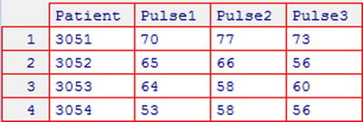
Figure 3-3. pulserates dataset giving the pulse rates of four patients, measured in triplicate (see Appendix C for more details)
Suppose that you want to calculate a new variable giving the mean pulse for each patient. You can create the new variable (shown in Figure 3-4) with the command:
> pulserates$Mean.Pulse<-apply(pulserates[2:4], 1, mean)
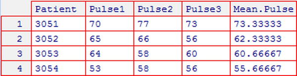
Figure 3-4. pulserates dataset with the new Mean.Pulse variable
Notice that bracket notation is used to select column numbers 2 to 4. (The “Data frames” section in Chapter 1 gives more details on using bracket notation.)
The second argument allows you to specify whether the summary should be calculated for each row (by setting it to 1) or each column (by setting it to 2). To create a new variable, set it to 1.
You can substitute the mean function with any univariate statistical summary function that gives a single value as output, such as sd or max. Table 5-1 gives a list of these (use only those marked with an asterisk).
Dividing a Continuous Variable into Categories
Sometimes you may want to create a new categorical variable by classifying the observations according to the value of a continuous variable.
For example, consider the people dataset shown in Figure 3-1 Suppose that you want to create a new variable called Height.Cat, which classifies the people as “Short”, “Medium”, and “Tall” according to their height. People less than 160 cm tall are classified as Short, people between 160 cm and 180 cm tall are classified as Medium, and people greater than 180 cm tall are classified as Tall.
You can create the new variable with the cut function:
> people$Height.Cat<-cut(people$Height, c(150, 160, 180, 200), c("Short", "Medium", "Tall"))
Figure 3-5 shows the people dataset with the new Height.Cat variable.
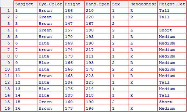
Figure 3-5. The people dataset with the new Height.Cat variable
When using the cut function, the numbers of group boundaries (in this example four) must be one more than the number of group names (in this example three). If a data value is equal to one of the boundaries, it is placed in the category below. Make sure your categories cover the whole range of the data values; otherwise, the new variable will have missing values. In this example, there is one observation (subject 3) that does not fall in to any of the categories that have been defined, so has a missing value for the Height.Cat variable.
If you prefer, you can specify the number of categories and let R determine where the boundaries should be. R divides the range of the variable to create evenly sized categories. For example, this command shows how you would split the Height variable into three evenly sized categories:
> people$Height.Cat<-cut(people$Height, 3, c("Short", "Medium", "Tall"))
Any variables you create with the cut function are automatically assigned the factor class.
![]() Note Always consider carefully whether you really need to divide a numeric variable into categories. Numeric variables contain more information than categorical variables, so it is often wisest to include the original numeric variable directly in your statistical models where possible.
Note Always consider carefully whether you really need to divide a numeric variable into categories. Numeric variables contain more information than categorical variables, so it is often wisest to include the original numeric variable directly in your statistical models where possible.
As explained under “Variable classes,” factor variables are suitable for holding categorical data. To change the class of a variable to factor, use the as.factor function:
> people$Sex<-as.factor(people$Sex)
A factor variable has a number of levels, which are all of the unique values that the variable takes (i.e., all of the possible categories). To view the levels of a factor variable, use the levels function:
> levels(people$Sex)
[1] "1" "2"
Because the level names will appear on any plots and statistical output that you create based on the variable, it is helpful if they are meaningful and attractive. You can change the names of the levels:
> levels(people$Sex)<-c("Male", "Female")
You must give the same number of names as there are levels of the factor, and enter the new names in corresponding order.
You can also combine factor levels by renaming them. Consider the Eye.Color variable in the people dataset. Using the levels function, you can see that there is an extra level resulting from a spelling variation:
> levels(people$Eye.Color)
[1] "Blue" "brown" "Brown" "Green"
To rename the second factor level so that it has the correct spelling, use the command:
> levels(people$Eye.Color)[2]<-"Brown"
When the factor levels are viewed again, you can see that the two levels have been combined:
> levels(people$Eye.Color)
[1] "Blue" "Brown" "Green"
You can change the order of the levels with the relevel function. For example, to make Brown the first level of the Eye.Color variable, use the command:
> people$Eye.Color<-relevel(people$Eye.Color, "Brown")
The order of the factor levels is important, because if you include the factor in a statistical model, R uses the first level of the factor as the reference level. You will learn more about this in Chapter 11.
Manipulating Character Variables
R has a number of functions for manipulating character strings. Three of the most useful are paste (for concatenating strings), substring (for extracting a substring), and grep (for searching a string). These are demonstrated in the following subsections.
Concatenating Character Strings
The paste function allows you to create new character variables by pasting together existing variables (of any class) and other characters.
Consider the fruit dataset shown in Figure 3-6, which gives prices for a selection of fruit.

Figure 3-6. fruit dataset giving U.K. fruit prices for August 2012 (see Appendix C for more details)
Suppose that you want to create a new variable giving a price label for each of the fruit. The label should have the product description, price with pound sign, and sale unit. You can create the new variable (shown in Figure 3-7) with the command:
> fruit$Label<-paste(fruit$Product, ": £", format(fruit$Price, trim=T, digits=2), " ", fruit$Unit, sep="")
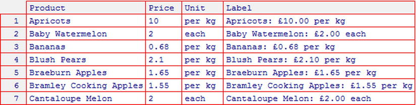
Figure 3-7. fruits dataset with new Label variable
By default, the paste function inserts a space between each of the components being pasted together. In this example, sep="" has been added to prevent this, so that spaces are not inserted in unwanted places such as between the pound sign and the price. Instead, spaces have been inserted manually where required, placed between quotation marks. You can also use the sep argument to specify another keyboard symbol to use as a separator.
Notice that the format function has been used to ensure that the fruit prices are always displayed to two decimal places.
Extracting a Substring
The substring function allows you to create a new variable by extracting a section of characters from an existing variable.
Consider the flights dataset shown in Figure 3-8a. The Flight.Number variable gives flight numbers that begin with a two-letter prefix, indicating which airline the flight is operated by. Suppose that you wish to create two new variables, one named Airline giving the two-letter airline prefix and another named Ref giving the number component, as shown in Figure 3-8b.

Figure 3-8. flights dataset giving details of flights from Southampton Airport (see Appendix C for more details)
When using the substring function, give the positions within the character string of the first and last characters you want to extract. So to extract the first two characters from the Flight.Number variable to create the Airline variable, use the command:
> flights$Airline<-substring(flights$Flight.Number, 1, 2)
You can also give a starting position only, and the remainder of the string is extracted. So to create the Ref variable, use the command:
> flights$Ref<-substring(flights$Flight.Number, 3)
Note that although the new Ref variable contains numbers, it still has the character class because it was created with the substring function. If you wanted to use it as a numeric variable, you can convert it with the as.numeric function as described under “Variable classes.”
Searching a Character Variable
The grep function allows you to search a character string for a search term.
Consider the customers dataset shown in Figure 3-9. Suppose that you want to identify all of the customers who live in the city of Reading.
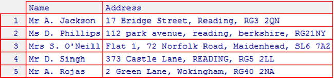
Figure 3-9. The customers dataset (see Appendix C for more details)
This command searches the Address variable for the term “reading”:
> grep("reading", customers$Address)
[1] 2
R outputs the number 2 to indicate that observation number 2 contains the term “reading”.
Notice that R has only returned one result because the search in case sensitive, so that “Reading” and “READING” are not considered matches to the search term “reading”. To change this, set the ignore.case argument to T:
> grep("reading", customers$Address, ignore.case=T)
[1] 1 2 4
Instead of displaying the observation numbers, you can save them to an object. This allows you to create a new dataset containing only the observations that matched the search term:
> matches<-grep("reading", customers$Address, ignore.case=T)
> reading.customers<-customers[matches,]
R has special date and date-time variable classes that make this type of data easier to work with. When you import a dataset, R does not automatically recognize date variables. Instead, they are assigned one of the other classes according to their contents. You can convert these variables with the as.Date and strptime functions.
For variables containing just dates (without times), use the as.Date function to convert the variable to the date class. The command takes the form:
>dataset$variable<-as.Date(dataset$variable, "format")
where "format" tells R how to read the dates. R uses a special notation for specifying the format of a date, shown in Table 3-1.
Table 3-1. The Most Commonly Used Symbols for Date-Time Formats. Enter help(strptime) to View a Complete List
Symbol |
Meaning |
Possible values |
|---|---|---|
%d |
Day of the month |
01 to 31, or 1 to 31 |
%m |
Month number |
01 to 12 |
%b |
Three letter abbreviated month name |
Jan, Feb, Mar, Apr, etc. |
%B |
Full month name |
January, February, March, April, etc. |
%y |
Two-digit year |
00 to 99, e.g., 10 for 2010 |
%Y |
Four-digit year |
e.g., 2004 |
%H |
Hour in 24-hour format |
0 to 23, e.g. 19 for 7pm |
%M |
Minute past the hour |
00 to 59 |
%S |
Seconds past the hour |
00 to 59 |
%I |
Hour in 12-hour format |
01 to 12 |
%p |
AM or PM |
AM or PM |
Consider the Date variable in the coffeeshop dataset, shown in Figure 3-10. The variable has dates in the format dd/mmm/yyyy.

Figure 3-10. coffeeshop dataset (see Appendix C for more details)
To convert the variable to the date class, use the command:
> coffeeshop$Date<-as.Date(coffeeshop$Date, "%d/%b/%Y")
The format %d/%b/%Y tells R to expect a day (%d), three-letter month name (%b), and four-digit year (%Y), separated by forward slashes. The format must be enclosed in quotation marks.
There are two date formats that R recognizes without you needing to specify them, which are yyyy-mm-dd and yyyy/mm/dd. If your dates are in either of these formats, then you don’t need to give a format when using the as.Date function.
For variables containing dates with time information, use the strptime function to convert the variable to the POSIXlt class.
For example, suppose that you want to create a new date-time variable from the Date and Time variables in the flights dataset (refer to Figure 3-6).
Before you can create a date-time variable, you will need to combine the two variables to create a single character variable using the paste function (refer to the “Concatenating character strings” section):
> flights$DateTime<-paste(flights$Date, flights$Time)
Once the date and time are together in the same character string, you can use the strptime function to convert the variable class. The strptime function is used in the same way as the as.Date function:
> flights$DateTime<-strptime(flights$DateTime, "%d/%m/%Y %H:%M")
Once your variable has the date or POSIXlt class, you can perform a number of date-related operations using functions designed for these variable classes.
For example, to find the length of the time interval between two dates or date-times, use the difftime function:
>dataset$duration<-difftime(dataset$enddate,dataset$startdate, units="hours")
Options for the units argument are secs, mins, hours, days (the default), and weeks.
To compare a date variable with the current date (e.g., to calculate an age), use the Sys.Date function:
>dataset$age<-difftime(Sys.Date(),dataset$dob)
You can use arithmetic operators to add or subtract days (for date variables) or seconds (for POSIXlt variables). For example, to find the date one week before a given date:
>dataset$newdatevar<-dataset$datevar-7
To find which day of the week a date falls on, use the weekdays function. There are also similar functions called months and quarters:
> coffeeshop$Day<-weekdays(coffeeshop$Date)
The round function can also be used with date-time variables. Specify one of the time units, secs, mins, hours, or days:
> round(flights$DateTime, units="hours")
You can create a character variable from a date variable with the format function. Specify how you want R to display the date using the format symbols given in Table 3-1:
>dataset$charvar<-format(dataset$datevar, format="%d.%m.%Y")
Adding and Removing Observations
You can use the data editor to add new observations to a data frame, and bracket notation to remove specific observations. R has a special function called unique for removing duplicates.
If you want to remove all of the observations that match specified criteria or belong to a particular group, use the subset function as explained under “Selecting a subset according to selection criteria” later in this chapter.
The simplest way to add additional observations to a dataset is with the data editor, which you can open with the command:
> fix(dataset)
When the editor window opens, type the values for the new observation into the first empty row beneath the existing data. If any of the values are missing, leave the relevant cell empty. When you have finished adding new values, close the data editor to apply the changes.
Removing Specific Observations
The simplest way to remove individual observations from a dataset is using bracket notation (see the “Data Frames” section in Chapter 1). For example, to remove observation numbers 2, 4, and 7, use the command:
>dataset<-dataset[-c(2,4,7),]
Be careful to include the comma before the closing bracket; otherwise, you will remove columns rather than rows.
Remember that you can also use the colon symbol (:) to select a range of consecutive observations. For example, to remove observation numbers 2 to 10, use the command:
>dataset<-dataset[-c(2:10),]
Removing Duplicate Observations
To remove duplicates observations from a dataset, use the unique function.
>dataset<-unique(dataset)
To save the duplicates to a separate dataset before removing them, use the duplicated function:
>dups<-dataset[duplicated(dataset),]
Selecting a Subset of the Data
Observations can be selected according to selection criteria based on properties of the data, or randomly to form a random sample.
Selecting a Subset According to Selection Criteria
Sometimes you may need to select a subset of a dataset containing only those observations that match certain criteria, such as belonging to a particular category or where the value of one of the numeric variables falls within a given range. You can do this with the subset function. The command takes the general form:
> subset(dataset,condition)
For example, to select all of the observations from the people dataset where the value of the Eye.Color variable is Brown, use the command:
> subset(people, Eye.Color=="Brown")
   Subject  Eye.Color  Height  Hand.Span  Sex  Handedness
1        1      Brown     186        210    1           R
3        3      Brown     147        167    2
5        5      Brown     170        193    1           R
11      11      Brown     163        223    1           R
16      16      Brown     173        196    1           R
Notice that you must use two equals signs rather than one.
To save the selected observations to a new dataset, assign the output to a new dataset name:
> browneyes<-subset(people, Eye.Color=="Brown")
To select all the observations for which a variable takes any one of a list of values, use the %in% operator. For example, to select all observations where Eye.Color is either Brown or Green, use the command:
> subset(people, Eye.Color %in% c("Brown", "Green"))
   Subject  Eye.Color  Height  Hand.Span  Sex  Handedness
1        1      Brown     186        210    1           R
2        2      Green     182        220    1           R
3        3      Brown     147        167    2
4        4      Green     157        180    2           L
5        5      Brown     170        193    1           R
11      11      Brown     163        223    1           R
15      15      Green     160        190    2
16      16      Brown     173        196    1           R
To select observations to exclude instead of to include, replace == with != (which mean “not equal to”). For example, to exclude all observations where the value of Eye.Color is equal to "Blue", use the command:
> subset(people, Eye.Color!="Blue")
Observations can also be selected according to the value of a numeric variable. For example, to select all observations from the people dataset where the Height variable is equal to 169, use the command:
> subset(people, Height==169)
    Subject  Eye.Color  Height  Hand.Span  Sex  Handedness
6         6       Blue     169        190    2           L
Notice that quotation marks are not required for numeric values.
With numeric variables, you can also use relational operators to select observations. For example, to select all observations for which the value of the Height variable is less than 165, use the command:
> subset(people, Height<165)
     Subject  Eye.Color  Height  Hand.Span  Sex  Handedness
3          3      Brown     147        167    2
4          4      Green     157        180    2           L
11        11      Brown     163        223    1           R
15        15      Green     160        190    2
Other relational operators you could use are > (greater than), >= (greater than or equal to) and <= (less than or equal to).
You can combine two or more conditions using the AND operator (denoted &) and the OR operator (denoted |). When two criteria are joined with the AND operator, R selects only those observations that meet both conditions. When they are joined with the OR operator, R selects the observations that meet either one of the conditions, or both.
For example, to select observations where Eye.Color is BrownandHeight is less than 165, use the command:
> subset(people, Eye.Color=="Brown" & Height<165)
     Subject  Eye.Color  Height  Hand.Span  Sex  Handedness
3          3      Brown     147        167    2
11        11      Brown     163        223    1           R
As well as selecting a subset of observations from the dataset, you can also use the select argument to select which variables to keep.
> subset(people, Height<165, select=c(Hand.Span, Height))
     Hand.Span  Height
3          167     147
4          180     157
11         223     163
15         190     160
Another way to subset a dataset is using bracket notation. For example, this command selects only those people with brown eyes:
> people[people$Eye.Color=="Brown",]
Note that it is not always necessary to subset a dataset before performing analysis. Many analysis functions have a subset argument within the function. This allows you to perform the analysis for a subset of the data. For example, this command creates a scatter plot of height against hand span, showing only males (i.e., where Sex is equal to 2):
> plot(Height~Hand.Span, people, subset=Sex==2)
You will learn more about scatter plots in Chapter 8.
Selecting a Random Sample from a Dataset
To select a random sample of observations from a dataset, use the sample function. For example, the following command selects a random sample of 50 observations from a dataset named dataset and saves them to new dataset named sampledata:
>sampledata<-dataset[sample(1:nrow(dataset), 50),]
By default, the sample function samples without replacement, so that no observation can be selected more than once. For this reason, the sample size must be less than the number of observations in the dataset. To sample with replacement, set the replace argument to T:
>sampledata<-dataset[sample(1:nrow(dataset), 50, replace=T),]
You can use the order function to sort a dataset. For example, to sort the people dataset by the Hand.Span variable, use the command:
> people<-people[order(people$Hand.Span),]
     Subject  Eye.Color  Height  Hand.Span  Sex  Handedness
3          3      Brown     147        167    2
10        10       Blue     166        178    2           R
4          4      Green     157        180    2           L
6          6       Blue     169        190    2           L
15        15      Green     160        190    2
5          5      Brown     170        193    1           R
9          9       Blue     166        193    2           R
16        16      Brown     173        196    1           R
1          1      Brown     186        210    1           R
8          8       Blue     173        211    1           R
13        13       Blue     176        214    1
7          7      Brown     174        217    1           R
14        14       Blue     183        218    1           R
2          2      Green     182        220    1           R
11        11      Brown     163        223    1           R
12        12       Blue     184        225    1           R
To sort in decreasing instead of ascending order, set the decreasing argument to T:
> people<-people[order(people$Hand.Span, decreasing=T),]
You can also sort by more than one variable. To sort the dataset first by Sex and then by Height, use the command:
> people<-people[order(people$Sex, people$Height),]
Summary
You should now be able to prepare your dataset by creating any new variables required for your analysis, removing irrelevant data, and tidying the final dataset.
This table shows the most important commands covered in this chapter.
Task |
Command |
|---|---|
Rename variable |
names(dataset)[n]<-"Newname" |
View variable class |
class(dataset$variable) |
Change variable class to numeric |
dataset$var1<-as.numeric(dataset$var1) |
Change variable class to factor |
dataset$var1<-as.factor(dataset$var1) |
Change variable class to character |
dataset$var1<-as.character(dataset$var1) |
Change variable class to date |
dataset$var1<-as.Date(dataset$var1, "format") |
Copy variable |
dataset$var2<-dataset$var1 |
Divide variable into categories |
dataset$factor1<-cut(dataset$var1, c(1,2,3,4), c("Name1", "Name2","Name3")) |
Rename factor level |
dataset$variable)[n]<-"Newname" |
Reorder factor levels |
dataset$variable, "Level1") |
Join two character strings |
dataset$var3<-paste(dataset$var1,dataset$var2) |
Extract a substring |
dataset$var2<-substring(dataset$var1,first,last) |
Search character variable |
grep("search term",dataset$variable) |
Remove cases |
dataset<-dataset[-c(2,4,7),] |
Remove duplicates |
dataset<-unique(dataset) |
Select subset |
subset(dataset,variable=="value") |
Select random sample |
newdataset<-dataset[sample(1:nrow(dataset),samplesize),] |
Sort dataset |
dataset<-dataset[order(dataset$variable),] |
In Chapter 4, you will learn how to make more complex changes to datasets, including combining two or more datasets and changing the structure of the data.