
![]()
Basic Programming with R
As well being a statistical computing environment, R is also a programming language. The topic of R programming is beyond the scope of this book. However, this chapter gives a brief introduction to basic programming and writing your own functions.
When programming, use a script file so that you can edit your code easily. Remember to add plenty of comments with the hash symbol (#), so that your script can be understood by others or by yourself at a later date.
Creating New Functions
Throughout this book, you will have used many of R’s built-in functions, but it is also possible to create your own. Creating your own function allows you to neatly bundle together a group of commands that perform a specific task that you want to use repeatedly.
To create a new function, the script takes the following general form:
functionname<-function(arg1name,arg2name, ..., argNname) {

     command(s)

     return(outputvalue)
}
All of the indentation and additional blank lines are optional, but they help to show the hierarchy of the program and are considered good programming practice.
The first line determines the name of the function and the names of the input arguments. You can include as many arguments as required, or none at all. Optionally, you can assign default values to the arguments:
functionname<-function(arg1name=value1,arg2name=value2, ...,argNname=valueN) {

     command(s)

     return(outputvalue)
}
This first line of the script ends with an opening curly bracket. After this is where the main content of the function begins. Generally, this is a set of commands that manipulate the input arguments in some way, or perform calculations from them, in order to create an output. The commands can make use of existing functions, including any that you have written yourself. Note that any objects that you create within a function exist only inside the function and are not saved to the workspace.
The return function determines the output of the function, which is either displayed in the console or assigned to an object whenever the function is used. It can either be a literal value such as a number or character string, or a it can be a vector, data frame or any other type of object.
Instead of using the return function in the final command, you can use the print function, which always displays the output in the console window even if the output is assigned to an object. Alternatively, you may want to create a function that produces a plot instead of giving an output value. In this case, the final command would be plot or another plotting function.
Finally, the script ends with a closing curly bracket.
Once you have written your function and run the script, the function is saved to the workspace as an object and is available to use for as long as the current workspace is loaded. You can use it just like a built-in function:
>functionname(value1,value2, ..., valueN)
EXAMPLE B-1. A FUNCTION FOR FINDING THE CUBE ROOT OF A VALUE
This script creates a simple function, which takes a single value as input and calculates the cube root:
cube.root<-function(x) {
y<-x^(1/3)
return(y)
}
Try entering the function into a script file and running the program. Recall that to run a script file in the Windows environment, you must highlight the text that you want to run and then right-click and select Run line or selection, as shown in Figure B-1. Alternatively, you can highlight the text and press the Run button. Mac users should highlight the text and then press Cmd+Return.
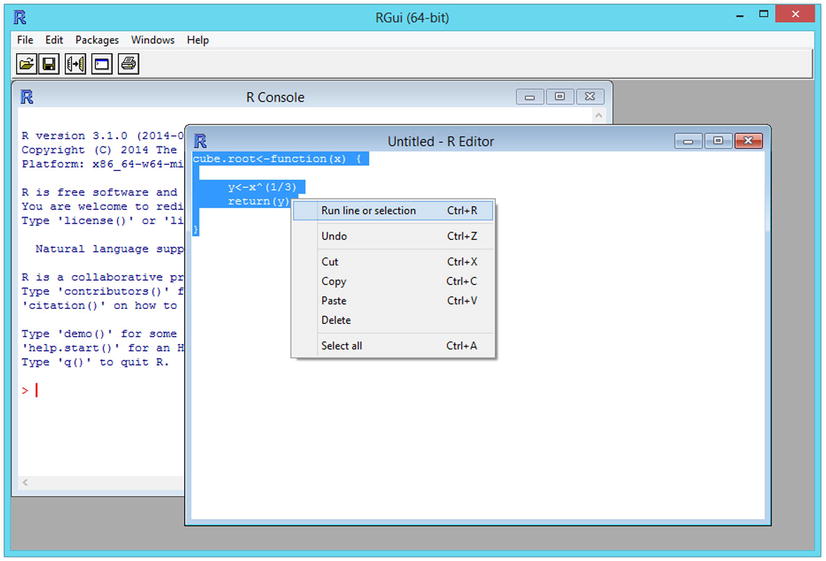
Figure B-1. Entering a program into a script file and running (Windows)
Once you have written the function and run the script, the cube.root function is available to use:
> cube.root(5)
[1] 1.709976
EXAMPLE B-2. A FUNCTION FOR CALCULATING THE HYPOTENUSE OF A TRIANGLE
This script creates a simple function, which calculates the length of the hypotenuse of a triangle, given the lengths of the other two sides (recall that the formula is c2=a2+b2):
hypot<-function(a=2, b=3) {
c=sqrt(a^2+b^2)
return(c)
}
Once the function is written and the script run, you can use it:
> hypot(6, 7)
[1] 9.219544
As the arguments have been given default values, the function still works if one or both of them are missing:
> hypot(b=2)
[1] 2.828427
EXAMPLE B-3. A FUNCTION THAT CREATES A HISTOGRAM OF RANDOM NUMBERS
This script creates a function that generates a specified amount of random numbers from a standard normal distribution and plots them in a histogram:
randhist<-function(n) {
vector1<-rnorm(n) # Generate n random numbers
# Plot random numbers in a histogram, add a title and remove the x-axis label:
hist(vector1, main="Histogram of a random sample from a
standard normal distribution",
xlab="")
}
Once the function is written and the script has been run, you can use it:
> randhist(50)
The result should be similar to Figure B-2.
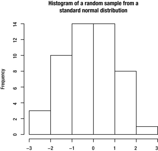
Figure B-2. Histogram created by the randhist function
Consider the cube.root function created in Example B-1. If you try to input a negative number, you get the result shown here.
> cube.root(-5)
[1] NaN
It would be nice if the function could return an error message to explain to the user what went wrong. In order to do this, the function would need to behave differently depending on whether the user inputs a positive number or a negative number. This is what a conditional statement allows you to do.
A conditional statement allows you to perform a command or set of commands only under certain circumstances (called the condition). Conditional statements add flexibility to your functions, as they allow the function to behave in different ways depending on the input.
There are a few types of conditional statement that allow you to do slightly different things. Before looking at these, you need to understand conditions and how they are constructed in R.
Conditions
In programming, a condition is an expression that can be either true or false. For example, the condition '4<5' (4 is less than 5) is true, whereas the condition '5==8' (5 is equal to 8) is false.
If you enter a condition at the command prompt, R tells you whether it is true or false:
> 6>8
[1] FALSEA condition must contain at least one comparison operator (also known as a relational operator). In the preceding example, the comparison operator is > (greater than). Table B-1 gives a list of comparison operators that you can use to form conditions.
Table B-1. Comparison operators
Operator |
Meaning |
|---|---|
== |
Equal to |
< |
Less than |
<= |
Less than or equal to |
> |
Greater than |
>= |
Greater than or equal to |
%in% |
In |
The %in% operator compares a single value with all members of a vector:
> vector1<-c(4,2,1,6)
> 2 %in% vector1
[1] TRUEConditions containing only constant values are not very useful because we already know in advance whether they are true or false. More useful are conditions that include objects, such as 'object1<5' (the value of object1 is less than 5). Whether or not this condition is true depends on the value of object1:
> object1<-4
> object1<5
[1] TRUEYou can join two or more conditions to form a larger one, using the OR and AND operators.
The AND operator is denoted &. When two expressions are joined with the AND operator, both must be true in order for the whole condition to be true. For example, this condition is false because only one of the expressions is true:
> 3<5 & 7<5
[1] FALSEThis statement is true because both of the expressions are true:
> 3<5 & 7>5
[1] TRUEThe OR operator is denoted |. When two expressions are joined with the OR operator, the overall condition is true if either one or both of the expressions are true. For example, this condition is true because one of the expressions is true:
> 3<5 | 7<5
[1] TRUEThe condition is also true when both expressions are true:
> 3<5 | 7>5
[1] TRUEYou can negate a condition with the ! operator. This reverses the result of the condition:
> !3<5
[1] FALSEIf the condition is complex, you can use brackets to negate the entire condition:
> !(3<5 & 7<5)
[1] TRUEThe simplest form of conditional statement is the if statement. The if statement consists of a condition and a command. When R runs an if statement, it first checks whether the condition is true or false. If the condition is true, it runs the command and if it is false it does not. The general form for the statement is shown here:
if (condition)command
You can also include a group of several commands in an if statement, by placing them between curly brackets:
if (condition) {

     commands to be performed if condition is true

}
The if statement is very useful as part of a function, as illustrated in the following examples.
EXAMPLE B-4. FUNCTION FOR CALCULATING THE CUBE ROOT OF A VALUE (UPDATED)
This script creates an updated version of the cube.root function from Example B-1, which returns a warning message if the user inputs a negative number. Notice that it uses the warning function, which prints warning messages. R also has a function called stop, which causes the function to abort and prints an error message:
cube.root<-function(x) {
y<-x^(1/3) # Calculate the cube root
# If user enters a negative number, print warning message:
if (x<0) warning("Cannot calculate cube root of negative number")
return(y)
}
The updated function now returns a warning message only if the user input a negative number:
> cube.root(5)
[1] 1.709976> cube.root(-5)
[1] NaN
Warning message:
In cube.root(-5) : Cannot calculate cube root of negative number
EXAMPLE B-5. A FUNCTION FOR CALCULATING BODY MASS INDEX
A person’s body mass index (BMI) is calculated from his or her height in meters and weight in kilograms using the formula:
BMI=Weight/Height2
If imperial measurements are used (height in inches and weight in pounds), the formula is:
BMI=Weight×702/Height2
This script creates a function to calculate the BMI from a height and weight. By default, the function calculates the BMI, assuming that the metric measurements have been supplied. If the user sets the units argument to "imperial", the function makes the appropriate adjustment for imperial measurements. Notice the use of the if statement (shown in bold) to control whether the adjustment is made:
bmi<-function(height, weight, units="metric") {
bmi<-weight/height^2 # Calculate BMI
if (units=="imperial") bmi<-bmi*702 # Adjust for imperial measurements
return(bmi)
}
Once the script has been run, you can use the function to calculate BMI using metric measurements:
> bmi(1.7, 70)
[1] 24.22145
or imperial measurements:
> bmi(66, 125, "imperial")
[1] 20.17332
The if/else statement extends the if statement to include a second command (or set of commands) to be performed if the condition is false. The general form is shown here:
if (condition)command1elsecommand2
You can include groups of commands between curly brackets:
if (condition) {

     commands to be performed if condition is true

} else {

     commands to be performed if condition is false

}
You can also extend the if/else statement to accommodate three or more possible outcomes:
if (condition1) command1 else if (condition2) command2 else command3
When running the statement, R begins by checking whether the first condition is true or false. If it is true, then the first command is run. If the first condition is false, then R proceeds to check the second condition. If the second condition is true then the second command is run. Otherwise, the final command is run.
EXAMPLE B-6. A FUNCTION FOR CLASSIFYING DATES
This script creates a function for classifying a date (given in the format ddmmmyyyy) as a weekend or a weekday:
day.type<-function(date) {
date1<-as.Date(date, "%d%b%Y") # Converts the date to date format
# Determines whether date is a weekend or weekday and prints the
# result:
if (weekdays(date1) %in% c("Saturday", "Sunday")) return ("Weekend") else
return("Weekday")
}
The function gives a different output depending on whether the input date is a weekend or a weekday:
> day.type("27JUN2014")
[1] "Weekday"
> day.type("28JUN2014")
[1] "Weekend"
EXAMPLE B-7. A FUNCTION FOR CLASSIFYING HEIGHTS
This script creates a function that takes a height in centimeters as input, and gives a height category as output. Heights below 140 cm are classified as 'Short', heights between 140 cm and 180 cm as 'Medium', and heights over 180 cm as 'Tall'.
heightcat<-function(height) {
if (height<140) return("Short") else if (height<180) return("Medium")
else return("Tall")
}
Once you have run the script, you can use the function:
> heightcat(136)
[1] "Short"
> heightcat(187)
[1] "Tall"
In some circumstances, you can use the switch function as a compact alternative to using if/else statements with many possible outcomes. The switch function selects between a list of alternative commands, each of which must return a single value. R compares the input with a list of options, and if it finds a match then it performs the corresponding command. The final command (which is optional) is performed if the input does not match any of the options:
> switch(input, option1=command1, option2=command2, option3=command3, command4)
There is another use of the switch function which takes an integer value as input, and outputs the corresponding value from a list of values:
> switch(input, value1, value2, value3, value4)
EXAMPLE B-8. FUNCTION TO PERFORM A SELECTED CALCULATION WITH TWO NUMBERS
This script creates a function that allows the user to give two numbers and a calculation type. The switch function is used to select from several commands, depending on which option the user selects:
calculator<-function(number1, number2, calctype="add") {
result<-switch(calctype,
"multiply"=number1*number2,
"divide"=number1/number2,
"add"=number1+number2,
"subtract"=number1-number2,
"exponent"=number1^number2,
"Invalid calculation type" # To cover all other possibilities
)
return(result)
}
Once the script has been run, you can use the function:
> calculator(2, 3, "divide")
[1] 0.6666667
> calculator(2, 3, "mean")
[1] "Invalid calculation type"
EXAMPLE B-9. FUNCTION FOR GIVING THE NAME OF THE DAY OF THE WEEK
This script creates a function named week.day that takes a number from 1 to 7 as input, and returns a character string giving the corresponding day of the week:
week.day<-function(daynum) {
dayname<-switch(daynum,
"Monday",
"Tuesday",
"Wednesday",
"Thursday",
"Friday",
"Saturday",
"Sunday"
)
return(dayname)
}
Once you have run the script, you can use it:
> week.day(2)
[1] "Tuesday"
Loops
Consider this script, which creates a function that takes a single number as input, multiplies it by each of the numbers 1 to 10, and displays the results in the console window:
times.table<-function(x) {

     result<-x*1                                   # Calculate result for x*1
     text<-paste(x, "times 1 equals", result)      # Create character string
                                                   # giving the result
     print(text)                                   # Print the result

     # Repeat for numbers 2 to 10:
     Result<-x*2
     text<-paste(x, "times 2 equals", result)
     print(text)

     result<-x*3
     text<-paste(x, "times 3 equals", result)
     print(text)

     # Continues to x*10

}
The function repeats the same three commands 10 times. It would be much more efficient if you could write the commands once and tell R to repeat them for each of the numbers 1 to 10. This is where loops become useful.
Loops allow you to repeat a command (or set of commands) a number of times. The two most important types of loop are the for loop and the while loop.
The for loop allows you to repeat a command or set of commands a prespecified number of times. The for loop takes the following general form:
for (i in startvalue:endvalue) command
You do not have to use i for the repetition number. Any valid object name can be used; however, i is conventional. The startvalue and endvalue can be either constant values or object names. R will repeat the command for each of the values from startvalue to endvalue.
Alternatively you can give a nonsequential vector as shown here, or you can even give a vector of character strings. R will repeat the command once for each of the values in the vector.
for i in c(5,7,8,2,11) command
You can also include a set of commands to be repeated by enclosing them within curly brackets:
for (i instartvalue:endvalue) {

     commands to be repeated

}
EXAMPLE B-10. FUNCTION FOR CALCULATING TIMES TABLES
This script creates a function that takes a single number as input, multiplies it by each of the numbers 1 to 10, and displays the results in the console window. The for loop (shown in bold) is used to repeat the calculation for each of the numbers 1 to 10:
times.table<-function(x) {
for (i in 1:10) {
result<-x*i # Calculate result
# Create character string giving the result:
text<-paste(x, "times", i, "equals", result)
print(text) # Print the result
}
}
Once the script has been run, you can use the function:
> times.table(5)
[1] "5 times 1 equals 5"
[1] "5 times 2 equals 10"
[1] "5 times 3 equals 15"
[1] "5 times 4 equals 20"
[1] "5 times 5 equals 25"
[1] "5 times 6 equals 30"
[1] "5 times 7 equals 35"
[1] "5 times 8 equals 40"
[1] "5 times 9 equals 45"
[1] "5 times 10 equals 50"
The while loop is suitable when you want to repeat a command or set of commands until a given condition is satisfied, and you don't know in advance how many repetitions will be required in order to achieve this. The general form for the while loop is shown here:
while (condition)command
To include a group of commands, use curly brackets:
while (condition) {

     commands to be repeated

}
The commands within the loop should do something that will affect whether or not the condition is true. For example, this script will keep printing the value of i until it reaches 10, at which point it will exit the loop:
i<-1
while (i<10) {

     print(i)
     i<-i+1

}
If the commands within the loop do not affect whether the condition is true, R will keep processing the commands infinitely. Consider this example:
b<-2
while (b<3) {
     print(b)
     a<-4
}
As the command within the loop is unrelated to the condition, the condition continues to be true each time the loop is repeated. This causes R to keep repeating the loop indefinitely and to stop responding. If you find R is stuck repeating a loop, press the Esc key to cancel the commands.
EXAMPLE B-11. FUNCTION FOR SIMULATING DIE ROLLS
The following script creates a function that simulates die rolls. The function keeps rolling imaginary dice until a six is rolled:
die.rolls<-function() {
roll<-0 # Create the object before using it in the loop
while (roll!=6) {
roll<-sample(1:6, 1) # Generate a random number between 1 and 6
print(roll)
}
}
Once the script is run, you can use the function:
> die.rolls()
[1] 1
[1] 1
[1] 5
[1] 6
> die.rolls()
[1] 1
[1] 3
[1] 3
[1] 1
[1] 3
[1] 6
Summary
You should now understand the basics of R programming and be able to create simple functions to perform routine tasks. You should be able to make your programs flexible by using appropriate statements to perform conditional execution, and use loops to perform sets of commands repeatedly.
This table summarizes the main statements covered.
Task |
General form |
|---|---|
Create a function |
functionname<-function(arguments) { |
if statement |
if (condition)command |
if/else statement |
if (condition) command1 else command2 |
if/else statement (extended) |
if (condition1) command1 else if (condition2) command2 else command3 |
switch function |
switch(input, value1, value2, valueN) |
switch(input, option1=command1, option2=command2, optionN=commandN) | |
for loop |
for (i in startval:endval) command |
while loop |
while (condition) command |