
![]()
Hypothesis Testing
Hypothesis testing is useful because it allow you to use your data as evidence to support or refute a claim, and helps you to make decisions. This chapter explains how to perform some of the most commonly used types of hypothesis test.
Most of the tests discussed in this chapter are used to compare sample means, but we will also look at tests for comparing sample variances. Both parametric and nonparametric tests are covered. Parametric tests make some assumptions about the distribution of the data, usually that the data follows a normal distribution. Nonparametric tests don’t make this kind of assumption, so are suitable in a wider range of situations.
You will learn how to:
- use a t-test to compare the means of two samples, or to compare one sample with a constant value
- perform a Wilcoxon rank-sum test (the non-parametric alternative to the t-test)
- use an analysis of variance to compare the means of three or more samples
- perform a Kruskal-Wallis test (the nonparametric alternative to the analysis of variance)
- perform pairwise comparisons using multiple comparison methods such as Tukey’s HSD, Bonferroni and pairwise Wilcoxon rank-sum test
- compare the variances of two or more samples using an F-test or Bartlett’s test
There are also several hypothesis tests that are covered in other chapters. The hypothesis test for correlation and the Shapiro-Wilk and Kolmogorov-Smirnov tests for fit to a distribution are covered in Chapter 5. Tests for tabular data, such as the chi-square test and Fisher’s test, can be found in Chapter 6.
This chapter uses the iris, PlantGrowth, and sleep datasets (included with R) and the bottles, brains, and grades1 datasets (available with the downloads for this book). To view more details about the dataset included with R, enter help(datasetname). For further details about all other datasets, see Appendix C.
HYPOTHESIS TESTS
A hypothesis test uses a sample to test hypotheses about the population from which the sample is drawn. This helps you make decisions or draw conclusions about the population. A hypothesis test has the following components:
Null hypothesis (denoted H0) is a hypothesis about the population from which a sample or samples are drawn. It is usually a hypothesis about the value of an unknown parameter such as the population mean or variance, e.g. H0: The population mean is equal to five. The null hypothesis is adopted unless proven false.
Alternative hypothesis (denoted H1 or HA) is the hypothesis that will be accepted if there is enough evidence to reject the null hypothesis. This is generally the inverse of the null hypothesis, e.g. H1: The population mean is not equal to five.
Test statistic is a statistic calculated from the sample values, which has a known distribution under the null hypothesis. It varies depending on the type of test and has no direct interpretation.
p-value gives the probability of observing the test statistic or something more extreme, assuming that the null hypothesis were true. If this is very small, then it suggests that the null hypothesis is not feasible, giving evidence in support of the alternative hypothesis.
Significance level (denoted α) is the cut-off point at which the null hypothesis is rejected. The significance level should be determined before beginning the test. Usually a significance level of 0.05 is used, but 0.01 and 0.1 are also popular choices. If a significance level of 0.05 is used, then we reject the null hypothesis in favor of the alternative hypothesis only if the p-value is less than 0.05. Otherwise, no conclusion is drawn. Choosing a significance level of 0.05 means that if the null hypothesis were true, there would be a 5% chance of incorrectly rejecting it (i.e., making a type I error).
The Student’s t-test is used to test hypotheses about the mean value of a population or two populations. A t-test is suitable if the data is believed to be drawn from a normal distribution. If the samples are large enough (i.e., at least 30 values per sample), then the t-test can be used even if the data is not normally distributed. This is because even if a random variable is not normally distributed, the mean values of a series of samples drawn from the distribution will tend to be normally distributed around the population mean, provided the samples are sufficiently large (the central limit theorem). If your data does not satisfy either of these criteria, then use the Wilcoxon rank-sum test instead, covered later in this chapter.
There are three types of t-test:
One-sample t-test is used to compare the mean value of a sample with a constant value denoted μ0. It has the null hypothesis that the population mean is equal to μ0, and the alternative hypothesis that it is not.
Two-sample t-test is used to compare the mean values of two independent samples, to determine whether they are drawn from populations with equal means. It has the null hypothesis that the two means are equal, and the alternative hypothesis that they are not equal.
Paired t-test is used to compare the mean values for two samples, where each value in one sample corresponds to a particular value in the other sample. It has the null hypothesis that the two means are equal, and the alternative hypothesis that they are not equal.
The t-test can also be performed with a one-sided alternative hypothesis, which is known as a one-tailed test. For a one-sample t-test, the one-sided alternative hypothesis is either that the mean is greater than μ0 or that the mean is less than μ0. For a two-sample or paired t-test, the one-sided alternative hypothesis is either that the mean of the first population is greater than the mean of the second population, or that the mean of the first population is less than the mean of the second population.
The following sections explain how to perform each type of t-test in R.
You can perform a one-sample t-test with the t.test function. To compare a sample mean with a constant value mu0, use the command:
> t.test(dataset$sample1, mu=mu0)
The mu argument gives the value with which you want to compare the sample mean. It is optional and has a default value of 0.
By default, R performs a two-tailed test. To perform a one-tailed test, set the alternative argument to "greater" or "less":
> t.test(dataset$sample1, mu=mu0, alternative="greater")
A 95% confidence interval for the population mean is included with the output. To adjust the size of the interval, use the conf.level argument:
> t.test(dataset$sample1, mu=mu0, conf.level=0.99)
EXAMPLE 10-1.
ONE-TAILED, ONE-SAMPLE T-TEST USING THE BOTTLES DATA
A bottle filling machine is set to fill bottles with soft drink to a volume of 500 milliliters. The actual volume is known to follow a normal distribution. The manufacturer believes the machine is under-filling bottles. A sample of 20 bottles is taken and the volume of liquid inside is measured. The results are given in the bottles dataset, which is available from the website.
To calculate the sample mean, use the command:
> mean(bottles$Volume)
[1] 491.5705
Suppose that you want to use a one-sample t-test to determine whether the bottles are being consistently under filled, or whether the low mean volume for the sample could be the result of random variation. A one-sided test is suitable because the manufacturer is specifically interested in knowing whether the volume is less than 500 milliliters. The test has the null hypothesis that the mean filling volume is equal to 500 milliliters, and the alternative hypothesis that the mean filling volume is less than 500 milliliters. A significance level of 0.01 is to be used.
To perform the test, use the command:
> t.test(bottles$Volume, mu=500, alternative="less", conf.level=0.99)
This gives the following output:
One Sample t-test
data: bottles$Volume
t = -1.5205, df = 19, p-value = 0.07243
alternative hypothesis: true mean is less than 500
99 percent confidence interval:
-Inf 505.6495
sample estimates:
mean of x
491.5705
From the output, we can see that the mean bottle volume for the sample is 491.6 ml. The one-sided 99% confidence interval tells us that mean filling volume is likely to be less than 505.6 ml. The p-value of 0.07243 tells us that if the mean filling volume of the machine were 500 ml, the probability of selecting a sample with a mean volume less than or equal to this one would be approximately 7%.
Because the p-value is not less than the significance level of 0.01, we cannot reject the null hypothesis that the mean filling volume is equal to 500 ml. This means that there is no evidence that the bottles are being underfilled.
You can use the t.test function to perform a two-sample t-test using data in both stacked and unstacked forms. Your data is in stacked form if all the data values are stored in one variable, and a second variable gives the name or number of the sample to which each observation belongs. Your data is in unstacked form if the values for each sample are held in separate variables. If you are unsure which form your data is in, consider Figure 10-1, which shows an example of a dataset in both stacked and unstacked form.
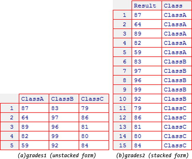
Figure 10-1. The same dataset in stacked and unstacked forms
To perform a two-sample t-test with data in stacked form, use the command:
> t.test(values~groups,dataset)
where values is the name of the variable containing the data values and groups is the variable containing the sample names. If the grouping variable has more than two levels, then you must specify which two groups you want to compare:
> t.test(values~groups,dataset,groups%in% c("Group1", "Group2"))
If your data is in unstacked form, use the command:
> t.test(dataset$sample1,dataset$sample2)
By default, R uses separate variance estimates when performing two-sample and paired t-tests. If you believe the variances for the two groups are equal, you can use the pooled variance estimate. An F-test or Bartlett’s test (see “Hypothesis Tests for Variance” later in this chapter) can help to determine whether this is the case. To use the pooled variance estimate, set the var.equal argument to T:
> t.test(values~groups,dataset, var.equal=T)
To perform a one-tailed test, set the alternative argument to "greater" or "less":
> t.test(values~groups,dataset, alternative="greater")
When the alternative argument is set to "greater", the alternative hypothesis for the test is that the mean for the first group is greater than the mean for the second group. If you are using stacked data, you may need to use the levels function to check which are the first and second groups (see “Working with Factor Variables” in Chapter 3). Similarly, setting it to "less" gives an alternative hypothesis that the mean for the first group is less than the mean for the second group.
A 95% confidence interval for the difference in means is included with the output. You can adjust the size of this interval with the conf.level argument:
> t.test(values~groups,dataset, conf.level=0.99)
EXAMPLE 10-2.
TWO-SAMPLE T-TEST USING THE IRIS DATA
Suppose that you wish to use a two-sample t-test to determine whether there is any real difference in mean sepal width for the Versicolor and Virginica species of iris. You can assume that sepal width is normally distributed, and that the variance for the two groups is equal. The null hypothesis for the test is that there is no real difference in mean sepal width for the two species, and the alternative hypothesis is that there is a difference.
The data is in stacked form, so perform the test with the command:
> t.test(Sepal.Width~Species, iris, Species %in% c("versicolor", "virginica"), var.equal=T)
The output is shown here.
Two Sample t-test
data: Sepal.Width by Species
t = -3.2058, df = 98, p-value = 0.001819
alternative hypothesis: true difference in means is not equal to 0
95 percent confidence interval:
-0.33028246 -0.07771754
sample estimates:
mean in group versicolor mean in group virginica
2.770 2.974
The 95% confidence interval for the difference is –0.33 to –0.08, meaning that the mean sepal width for the Versicolor species is estimated to be between 0.08 and 0.33 cm less than for the Virginica species.
The p-value of 0.001819 is less than the significance level of 0.05, so we can reject the null hypothesis that the mean sepal width is the same for the Versicolor and Virginica species in favor of the alternative hypothesis that the mean sepal width is different for the two species.
This example is continued in Example 10-9, where an F-test is used to check the assumption of equal variance (see “F-Test”).
You can perform a paired t-test by setting the paired argument to T. If your data is in stacked form, use the command:
> t.test(values~groups,dataset, paired=T)
Your data must have the same numbers of observations in each group, so that there is a one-to-one correspondence between the samples. R matches the first value from the first sample with the first value from the second sample.
For data in unstacked form, use the command:
> t.test(dataset$sample1,dataset$sample2, paired=T)
As for the two-sample test, you can adjust the test using the alternative, conf.level and var.equal arguments. So to perform a test with the alternative hypothesis that the mean for the first group is less than the mean for the second group, and that uses a pooled variance estimate, use the command:
> t.test(values~groups,dataset, paired=T, alternative="less", var.equal=T)
EXAMPLE 10-3.
PAIRED T-TEST USING THE BRAINS DATA
Consider the brains dataset shown in Figure 10-2, which gives brain volumes (in cubic centimetres) of the first and second-born twins for ten sets of monozygotic twins.
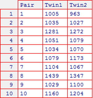
Figure 10-2. The brains dataset, giving brain volume data from the article “Brain Size, Head Size, and IQ in Monozygotic Twins,” by Tramo et al. (see Appendix C for more details)
Suppose that you wish to use a t-test to determine whether brain volume is related to birth order. Brain volume is assumed to follow a normal distribution. The data is naturally paired because the first twin from a birth corresponds to the second twin in the same birth, so a paired t-test is suitable. Because differences in either direction are of interest, a two-tailed test is used. The null hypothesis for the test is that there is no difference in mean brain volume for first- and second-born twins, and the alternative hypothesis is that the mean brain volume for first-born twins is different to that of second-born twins.
To perform the test, use the command:
> t.test(brains$Twin1, brains$Twin2, paired=T)
The output is shown here.
Paired t-test
data: brains$Twin1 and brains$Twin2
t = -0.4742, df = 9, p-value = 0.6466
alternative hypothesis: true difference in means is not equal to 0
95 percent confidence interval:
-49.04566 32.04566
sample estimates:
mean of the differences
-8.5
The mean difference in brain size is estimated at –8.5, meaning that the brain size of the first born twins was an average of 8.5 cubic centimeters less than that of their second born sibling. The confidence interval for the difference is –49 to 32 cubic centimeters.
The p-value of 0.6466 tells us that if the mean brain size for first- and second-born twins is the same, the probability of observing a difference equal or greater in magnitude to that in our sample is 65%. As the p-value is not less than the significance level of 0.05, the null hypothesis cannot be rejected. This means there is no evidence that brain size is related to birth order in twins.
The Wilcoxon rank-sum test (also known as the Mann-Whitney U test) allows you to test hypotheses about one or two sample means. It is a nonparametric alternative to the Student’s t-test, which is suitable even when the distribution of the data is unknown and the samples are small. In parallel with the t-test there are one-sample, two-sample and paired forms. The alternative hypothesis can be either two-sided or one-sided.
You can perform a Wilcoxon rank-sum test with the wilcox.test function. The commands are similar to those used to perform a t-test.
To perform a one-sample test, use the command:
> wilcox.test(dataset$sample1, mu=mu0)
To perform a two-sample test with data in stacked form, use the command:
> wilcox.test(values~groups, dataset)
If the grouping variable has more than two levels then you must specify which two you want to compare:
> wilcox.test(values~groups, dataset, groups%in% c(" Group1", " Group2"))
If your data is in unstacked form (with the values for each sample held in separate variables), use the command:
> wilcox.test(dataset$sample1, dataset$sample2)
For a paired test, set the paired argument to T:
> wilcox.test(values~groups, dataset, paired=T)
To perform a one-tailed test, set the alternative argument to "greater" or "less":
> wilcox.test(values~groups, dataset, alternative="greater")
By default, there is no confidence interval included with the output. To calculate a confidence interval for the population mean (for one-sample tests) or difference between means (for paired and two-sample tests), set the conf.int argument to T. The default size for the confidence intervals is 95%, but you can adjust this with the conf.level argument:
> wilcox.test(values~groups, dataset, conf.int=T, conf.level=0.99)
EXAMPLE 10-4.
PAIRED WILCOXON RANK-SUM TEST USING THE SLEEP DATA
Consider the sleep dataset, which is included with R. The data gives the results of an experiment in which 10 patients each took two different treatments and recorded the amount of additional sleep (compared to usual) that they experienced while receiving each of the treatments. The extra variable gives the increase in sleep (in hours per night), the group variable gives the treatment number (1 or 2), and the ID variable gives the patient number (1 to 10).
Suppose that you want to determine whether there is any real difference in the mean increase in sleep offered by the two treatments. A Wilcoxon rank-sum test is suitable because the distribution of additional sleep time is unknown, and the samples are small. A paired test is used because the additional sleep experienced by patient number x while taking drug 1 corresponds to the additional sleep experienced by patient number x while taking drug 2. The null hypothesis for the test is that there is no difference in mean additional sleep for the two treatments. The alternative hypothesis is that the mean additional sleep is different for the two treatments. A significance level of 0.05 will be used.
As the data is in stacked form, you can perform the test with the command:
> wilcox.test(extra~group, sleep, paired=T)
This gives the results:
Wilcoxon signed rank test with continuity correction
data: extra by group
V = 0, p-value = 0.009091
alternative hypothesis: true location shift is not equal to 0
Warning messages:
1: In wilcox.test.default(x = c(0.7, -1.6, -0.2, -1.2, -0.1, 3.4, 3.7, :
cannot compute exact p-value with ties
2: In wilcox.test.default(x = c(0.7, -1.6, -0.2, -1.2, -0.1, 3.4, 3.7, :
cannot compute exact p-value with zeroes
The p value of 0.009091 tells us that if the effect of both drugs were the same, there would be less than 1% chance of observing a difference in mean sleep increase as large as the one seen in this data. Because this is less than our significance level of 0.05, we can reject the null hypothesis that the additional sleep is the same for the two treatments. This means that there is evidence of a difference in effectiveness between the two treatments.
R has given a warning that there are ties in the data. This means that some observations have exactly the same value for the variable of interest, because the measurements have only been taken to one decimal place. For this reason, R is not able to calculate an exact p-value, and the results should be interpreted with caution. A more in-depth explanation of the effect of tied data on the Wilcoxon rank-sum test can be found on page 134 of Nonparametric Statistics for the Behavioural Sciences, Second Edition, by S. Siegel and N.J. Castellan (McGraw-Hill 1988).
An analysis of variance (or ANOVA) allows you to compare the means of three or more independent samples. It is suitable when the values are drawn from a normal distribution and when the variance is approximately the same in each group. You can check the assumption of equal variance with a Bartlett’s test (see “Hypothesis Tests for Variance” later in this chapter). The null hypothesis for the test is that the mean for all groups is the same, and the alternative hypothesis is that the mean is different for at least one pair of groups.
More complex models such as the two-way analysis of variance or the analysis of covariance are covered in Chapter 11.
You can perform an analysis of variance with aov function. Because the ANOVA is a type of general linear model, you could also use the lm or glm functions as explained in Chapter 11. However, the aov function presents the results more conveniently.
The command takes the form:
> aov(values~groups, dataset)
where values is the name of the variable that holds the data values and groups is the variable that identifies which sample each observation belongs to. If your data is in unstacked form (with the values for each sample held in separate variables) then you will need to stack the data beforehand, as explained in Chapter 4 under “Stacking Data.”
The results of the analysis consist of many components that R does not automatically display. If you save the results to an object as shown here, you can use further functions to extract the various elements of the output:
> aovobject<-aov(values~groups, dataset)
Once you have saved the results as an object, you can view the ANOVA table with the anova function:
> anova(aovobject)
To view the model coefficients, use the coef function:
> coef(aovobject)
To view confidence intervals for the coefficients, use the confint function:
> confint(aovobject)
EXAMPLE 10-5.
ANALYSIS OF VARIANCE USING THE PLANTGROWTH DATA
Consider the PlantGrowth dataset (included with R), which gives the dried weight of three groups of 10 batches of plants, where each group of 10 batches received a different treatment. The weight variable gives the weight of the batch and the groups variable gives the treatment received. Figure 10-3 shows a boxplot of the weight grouped by treatment group.
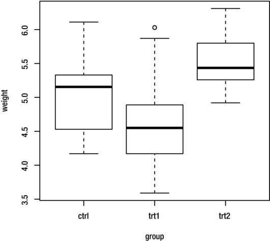
Figure 10-3. Boxplot of weight grouped by treatment group for the PlantGrowth dataset
You can see from the boxplot that there are some differences in plant growth (as measured by weight of batch) between the three groups. Suppose that you wish to perform an analysis of variance to determine whether these differences are statistically significant. You can assume that plant growth is normally distributed, and that the variance is the same for all three treatments. A significance level of 0.05 is used.
To perform the ANOVA and save the results to an object named plantanova, use the command:
> plantanova<-aov(weight~group, PlantGrowth)
To view the ANOVA table, use the command:
> anova(plantanova)
This gives the following output:
Analysis of Variance Table
Response: weight
Df Sum Sq Mean Sq F value Pr(>F)
group 2 3.7663 1.8832 4.8461 0.01591 *
Residuals 27 10.4921 0.3886
---
Signif. codes: 0 '***' 0.001 '**' 0.01 '*' 0.05 '.' 0.1 ' ' 1
We can see that the p-value for the group effect is 0.01591. This means that if the effect of all three treatments were the same, we would have less than 2% chance of seeing differences between groups as large or larger than this. As the p-value is less than the significance level of 0.05, we can reject the null hypothesis that the mean growth is the same for all treatments, in favor of the alternative hypothesis that the mean growth is different for at least one pair of treatments.
To see the size of the treatment effects, use the command:
> coef(plantanova)
(Intercept) grouptrt1 grouptrt2
5.032 -0.371 0.494
The output tells us that the control treatment gives an average weight of 5.032. The effect of treatment 1 (trt1) is to reduce weight by an average of –0.371 units compared to the control method, and the effect of treatment 2 (trt2) is to increase weight by an average of 0.494 units compared to the control method.
This example is continued in Example 10-7 (under “Tukey’s HSD Test”), where pairwise t-tests are used to further investigate the treatment differences, and in Example 10-10, where a Bartlett’s test is used to check the assumption of equal variance. Save the plantanova object, as it will be useful for these examples.
The Kruskal-Wallis test allows you to compare the mean values of three or more samples. It is a nonparametric alternative to the analysis of variance, which can be used when the distribution of the values is unknown.
You can perform a Kruskal-Wallis test with the kruskal.test function. To perform the test with stacked data, use the command:
> kruskal.test(values~groups, dataset)
where the values variable contains the data values and the groups variable indicates to which sample each observation belongs.
For unstacked data (with samples in separate variables), nest the variables inside the list function:
> kruskal.test(list(dataset$sample1, dataset$sample2, dataset$sample3))
EXAMPLE 10-6.
KRUSKAL-WALLIS TEST USING GRADES1 DATA
Consider the grades1 dataset, shown in Figure 10-4. It gives the test results (out of 100) of 15 students belonging to three different classes.
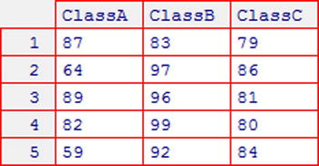
Figure 10-4. grades1 dataset (see Appendix C for more details)
Suppose that you want to use a Kruskal-Wallis test to determine whether there are any differences in the effectiveness of the teaching methods used by each of the three classes, as measured by the mean test results of the students. A significance level of 0.05 is used.
As the data is in unstacked form, you can perform the test with the command:
> kruskal.test(list(grades1$ClassA, grades1$ClassB, grades1$ClassC))
This gives the following output:
Kruskal-Wallis rank sum test
data: list(grades1$ClassA, grades1$ClassB, grades1$ClassC)
Kruskal-Wallis chi-squared = 6.6796, df = 2, p-value = 0.03544
From the output you can see that the p-value is 0.03544. As this is less than the significance level of 0.05, we can reject the null hypothesis that the mean score is equal for all classes. This means that there is evidence of a difference in effectiveness between the teaching methods used by the three classes.
This example is continued in Example 10-9, where pairwise Wilcoxon rank-sum tests are used to further investigate the differences between the three classes.
Multiple Comparison Methods
After performing an analysis of variance and finding that there are some differences between group means, you may want to perform a series of pairwise t-tests to identify differences between specific pairs of groups. However, when performing a large number of t-tests, the overall probability of incorrectly rejecting the null hypothesis for at least one of the tests (the type I error) is greater than the significance level used for the individual tests. Multiple comparison methods allow you to perform pairwise t-tests on three or more samples, while controlling the overall type I error.
There are a number of methods for performing multiple comparisons. Some of the most popular are the Tukey’s honestly significant difference (HSD) test and the Bonferroni test.
This following sections describe how to perform several prominent multiple comparison methods in R.
You can perform a Tukey’s HSD test with the TukeyHSD function. If you have previously performed an analysis of variance using the aov, lm, or glm functions and saved the results to an object (as explained previously in “Analysis of Variance”), use the function directly:
> TukeyHSD(aovobject)
If you don’t have an aov object and are using raw data, nest the aov function inside the TukeyHSD function:
> TukeyHSD(aov(values~groups, dataset))
The default overall confidence level is 0.95, but you can adjust it with the conf.level argument:
> TukeyHSD(aovobject, conf.level=0.99)
EXAMPLE 10-7.
TUKEY’S HSD TEST USING THE PLANTGROWTH DATA
In Example 10-5, an analysis of variance was used to help determine whether there are any differences in mean plant growth (measured by weight of batch) between the three treatment groups. The conclusion was that there is a difference in plant growth for at least one pair of treatments.
Suppose you wish to continue this analysis by using pairwise t-tests to determine which treatment groups have differences in plant growth. An overall significance level of 0.05 is used.
If you still have the plantanova aov object created in Example 10-5, you can perform the test with the command:
> TukeyHSD(plantanova)
If you no longer have the model object, you can perform the test from the raw data:
> TukeyHSD(aov(weight~group, PlantGrowth))
The output is shown here:
Tukey multiple comparisons of means
95% family-wise confidence level
Fit: aov(formula = weight ~ group, data = PlantGrowth)
$group
diff lwr upr p adj
trt1-ctrl -0.371 -1.0622161 0.3202161 0.3908711
trt2-ctrl 0.494 -0.1972161 1.1852161 0.1979960
trt2-trt1 0.865 0.1737839 1.5562161 0.0120064
The diff column shows the difference in sample means for the two groups, and the lwr and upr columns give a 95% confidence interval for the difference. The p adj column gives the p-value for a t-test between the two groups, adjusting for multiple t-tests.
Comparing the p-values to our significance level of 0.05, we can see that the comparison trt2-trt1 is statistically significant. This means that the plant growth for treatment 1 is significantly different from the growth for treatment 2. Treatment 1 and treatment 2 are not significantly different from the control.
Treatment 2 is estimated to give 0.865 units more growth than treatment 1. The 95% confidence interval for the difference in growth is 0.174 to 1.556.
The pairwise.t.test function allows you to perform pairwise t-tests using a number of other multiple comparison methods. To perform pairwise t-tests using the Bonferroni adjustment, use the command:
> pairwise.t.test( dataset$values, dataset$groups, p.adj="bonferroni")
Other possible options for the p.adj argument include holm (the default method), hochberg, and hommel. Enter help(p.adjust) to view a complete list.
EXAMPLE 10-8.
PAIRWISE COMPARISONS WITH BONFERRONI ADJUSTMENT USING THE PLANTGROWTH DATA
Continuing the PlantGrowth example, suppose that you wish to try performing pairwise t-tests using the Bonferroni adjustment for comparison:
> pairwise.t.test(PlantGrowth$weight, PlantGrowth$group, p.adj="bonferroni")
The results are shown here:
Pairwise comparisons using t tests with pooled SD
data: PlantGrowth$weight and PlantGrowth$group
ctrl trt1
trt1 0.583 -
trt2 0.263 0.013
P value adjustment method: bonferroni
The output shows p-values for each of the comparisons. From the output, we can see that the comparison of treatment 1 (trt1) and treatment 2 (trt2) has a p-value of 0.013, which is statistically significant at the 0.05 level. The comparison between the control and treatment 1, and between the control and treatment 2 were not statistically significant. This is consistent with the results of the Tukey’s HSD test in the previous example.
Pairwise Wilcoxon Rank-Sum Tests
There is also a function called pairwise.wilcox.test, which allows you to perform pairwise Wilcoxon rank-sum tests. This is useful for identifying differences between individual pairs of groups after performing a Kruskal-Wallis test (described earlier in this chapter).
To perform the test, use the command:
> pairwise.wilcox.test( dataset$values, dataset$groups)
As when performing pairwise t-tests, you can adjust the multiple comparison method with the p.adj argument.
Hypothesis Tests for Variance
A hypothesis test for variance allows you to compare the variance of two or more samples to determine whether they are drawn from populations with equal variance. The tests have the null hypothesis that the variances are equal and the alternative hypothesis that they are not. These tests are useful for checking the assumptions of a t-test or analysis of variance.
Two types of test for variance are covered in this section:
- F-test allows you to compare the variance of two samples. It is suitable for normally distributed data.
- Bartlett’s test allows you to compare the variance of two or more samples. It is suitable for normally distributed data.
The following sections explain how to perform both the F-test and Bartlett’s tests in R.
You can perform an F-test with the var.test function. If your data is in stacked form, use the command:
> var.test(values~groups, dataset)
If the groups variable has more than two levels, then you must specify which two you want to compare:
> var.test(values~groups, dataset,groups%in% c(" Group1", " Group2"))
For data in unstacked form (with the samples in separate variables), use the command:
> var.test( dataset$sample1, dataset$sample2)
EXAMPLE 10-10.
F-TEST USING THE IRIS DATASET
In Example 10-2, we used a t-test to compare the mean sepal width for the Versicolor and Virginica species of iris, using a pooled variance estimate. One of the assumptions made for this test was that the variance in sepal width is the same for both species.
Suppose that you want to use an F-test to help determine whether the variance in sepal width is the same for the two species. A significance level of 0.05 will be used.
To perform the test, use the command:
> var.test(Sepal.Width~Species, iris, Species %in% c("versicolor", "virginica"))
The output is shown here.
F test to compare two variances
data: Sepal.Width by Species
F = 0.9468, num df = 49, denom df = 49, p-value = 0.849
alternative hypothesis: true ratio of variances is not equal to 1
95 percent confidence interval:
0.5372773 1.6684117
sample estimates:
ratio of variances
0.9467839
The p-value of 0.849 is not less than the significance level of 0.05, so we cannot reject the null hypothesis that the variance for the two groups is equal. There is no evidence to suggest that the variance in sepal width is different for the Versicolor and Virginica species.
You can perform the Bartlett’s test with the bartlett.test function. If your data is in stacked form, use the command:
> bartlett.test(values~groups, dataset)
Unlike the F-test, the Bartlett’s test allows you to compare the variance of more than two groups. However, if required, you can still select a subset of groups to compare:
> bartlett.test(values~groups, dataset, groups%in% c("Group1", "Group2"))
If you have data in unstacked form (with the samples in separate variables), nest the variables inside the list function:
> bartlett.test(list( dataset$sample1, dataset$sample2, dataset$sample3))
EXAMPLE 10-11.
BARTLETT'S TEST USING THE PLANTGROWTH DATA
In Example 10-5, we used an analysis of variance to compare the mean weight of plant batches for the three treatment groups. One of the assumptions made for this test was that the variance in weight is the same for all treatment groups.
Suppose that you want to use Bartlett’s test to determine whether the variance in weight is the same for all treatment groups. A significance level of 0.05 will be used.
To perform the test, use the command:
> bartlett.test(weight~group, PlantGrowth)
This gives the output:
Bartlett test of homogeneity of variances
data: weight by group
Bartlett's K-squared = 2.8786, df = 2, p-value = 0.2371
From the output, we can see that the p-value of 0.2371 is not less than the significance level of 0.05. This means that we cannot reject the null hypothesis that the variance is the same for all treatment groups. This means that there is no evidence to suggest that the variance in plant growth is different for the three treatment groups.
Summary
You should now be able to compare the means of two samples using the t-test or Wilcoxon rank-sum test, and use an analysis of variance or Kruskal-Wallis test to compare the means of three or more samples. You should be able to perform pairwise comparisons of three or more groups using an appropriate method. Finally, you should be able to use an F-test or Bartlett’s test to compare the variances of two groups.
This table summarizes the most important commands covered.
Test Type |
Command |
|---|---|
One-sample t-test |
t.test(dataset$sample1, mu=mu0) |
Two-sample t-test |
t.test(values~groups, dataset) |
t.test(dataset$sample1, dataset$sample2) | |
Paired t-test |
t.test(values~groups, dataset, paired=T) |
t.test( dataset$sample1, dataset$sample2, paired=T) | |
One-sample Wilcoxon rank-sum test |
wilcox.test( dataset$sample1, mu=mu0) |
Two-sample Wilcoxon rank-sum test |
wilcox.test(values~groups, dataset) |
wilcox.test( dataset$sample1, dataset$sample2) | |
Paired Wilcoxon rank-sum test |
wilcox.test(values~groups, dataset, paired=T) |
wilcox.test( dataset$sample1, dataset$sample2, paired=T) | |
Analysis of variance |
aov(values~groups, dataset) |
Kruskal-Wallis test |
kruskal.test(values~groups, dataset) |
kruskal.test(list( dataset$sample1, dataset$sample2, dataset$sample3)) | |
Tukey’s HSD test |
tukeyHSD(aovobject) |
tukeyHSD(aov(values~groups, dataset)) | |
Pairwise t-tests |
paired.t.test( dataset$values, dataset$groups, method="bonferroni") |
Pairwise Wilcoxon rank-sum tests |
paired.wilcox.test( dataset$values, dataset$groups) |
F-test |
var.test(values~groups, dataset) |
var.test( dataset$sample1, dataset$sample2) | |
Bartlett’s test |
bartlett.test(values~groups, dataset) |
bartlett.test(list( dataset$sample1, dataset$sample2)) |
In the next chapter, we will look at how to build regression models and other types of general linear model.