Chapter 6
Storage
The storage component of any design of a vSphere environment is commonly regarded as one of the most crucial to overall success. It's fundamental to the capabilities of virtualization. Many of the benefits provided by VMware's vSphere wouldn't be possible without the technologies and features offered by today's storage equipment.
Storage technologies are advancing at a tremendous pace, particularly notable for such a traditionally staunch market. This innovation is being fueled by new hardware capabilities, particularly with widespread adoption of flash-based devices. Pioneering software advancements are being made possible via the commoditization of many storage array technologies that were previously only available to top-tier enterprise storage companies. When VMware launched vSphere 5, it was colloquially referred to as the storage release, due to the sheer number of new storage features and the significant storage improvements it brought.
The storage design topics discussed in this chapter are as follows:
- Primary storage design factors to consider
- What makes for an efficient storage solution
- How to design your storage with sufficient capacity
- How to design your storage to perform appropriately
- Whether local storage is still a viable option
- Which storage protocol you should use
- Using multipathing with your storage choice
- How to implement vSphere 5 storage features in your design
Dimensions of Storage Design
In the past, those who designed, built, configured, and most importantly, paid for server storage were predominantly interested in how much space they could get for their dollar. Servers used local direct attached storage (DAS), with the occasional foray into two node clusters, where performance was limited to the local bus, the speed of the disks, and the RAID configuration chosen. These configurations could be tweaked to suit all but the most demanding of server-room requirements. If greater performance was required, companies scaled out with multiple servers; or if they had the need (and the cash!), they invested in expensive dedicated Fibre Channel storage area network devices (SANs) with powerful array technologies. Times were relatively simple. CIOs cared about getting the most bang for their buck, and $/GB (cost per gigabyte) was what was on the storage planning table.
With the advent of virtualization, storage is now much more than just capacity. Arguably, the number of terabytes (TBs) that your new whizzy storage array can provide is one of the lesser interests when you're investigating requirements. Most shared storage units, even the more basic ones, can scale to hundreds of TBs.
Some of the intrinsic vSphere capabilities mean that storage is significantly more mobile than it was previously. Features such as Storage vMotion help abstract not just the server hardware but also the storage. Upgrading or replacing storage arrays isn't the thing of nightmares anymore; and the flexibility to switch in newer arrays makes the situation far more dynamic. Recent vSphere additions, such as Storage Distributed Resource Scheduler (Storage DRS) and Profile-Driven Storage, allow you to eke out even more value from your capital expenditure. Some of the innovative solutions around flash storage that are now available provide many options to quench virtualization's thirst for more input/output operations per second (IOPS).
Rather than intimidating or constraining the vSphere architect in you, this should open your mind to a world of new possibilities. Yes, there are more things to understand and digest, but they're all definable. Like any good design, storage requirements can still be planned and decisions made using justifiable, measurable analysis. Just be aware that counting the estimated number and size of all your projected VMs won't cut the mustard for a virtualized storage design anymore.
Storage Design Factors
Storage design comes down to three principle factors:
- Availability
- Performance
- Capacity
These must all be finely balanced with an ever-present fourth factor:
- Cost
Availability
Availability of your vSphere storage is crucial. Performance and capacity issues aren't usually disruptive and can be dealt with without downtime if properly planned and monitored. However, nothing is more noticeable than a complete outage. You can (and absolutely should) build redundancy in to every aspect of a vSphere design, and storage is cardinal in this equation. In a highly available environment, you wouldn't have servers with one power supply unit (PSU), standalone switches, or single Ethernet connections. Shared storage in its very nature is centralized and often solitary in the datacenter. Your entire cluster of servers will connect to this one piece of hardware. Wherever possible, this means every component and connection must have sufficient levels of redundancy to ensure that there are no single points of failure.
Different types of storage are discussed in this chapter, and as greater levels of availability are factored in, the cost obviously rises. However, the importance of availability should be overriding in almost any storage design.
Performance
Performance is generally less well understood than capacity or availability, but in a virtualized environment where there is significant scope for consolidation, it has a much greater impact. You can use several metrics, such as IOPS, throughput (measured in MBps), and latency, to accurately measure performance. These will be explained in greater depth later in the chapter.
This doesn't have to be the black art that many think it is—when you understand how to measure performance, you can use it effectively to underpin a successful storage design.
Capacity
Traditionally, capacity is what everyone thinks of as the focus for a storage array's principal specification. It's a tangible (as much as ones and zeros on a rusty-colored spinning disk can be), easily describable, quantitative figure that salesmen and management teams love. Don't misunderstand: it's a relevant design factor. You need space to stick stuff. No space, no more VMs. Capacity needs to be managed on an ongoing basis, and predicted and provisioned as required. However, unlike availability and performance, it can normally be augmented as requirements grow.
It's a relatively straightforward procedure to add disks and enclosures to most storage arrays without incurring downtime. As long as you initially scoped the fundamental parts of the storage design properly, you can normally solve capacity issues relatively easily.
Cost
Costs can be easy or difficult to factor in, depending on the situation. You may be faced with a set amount of money that you can spend. This is a hard number, and you can think of it as one of your constraints in the design.
Alternatively, the design may need such careful attention to availability, performance, and/or capacity that money isn't an issue to the business. You must design the best solution you can, regardless of the expense.
Although you may feel that you're in one camp or the other, cost is normally somewhat flexible. Businesses don't have a bottomless pit of cash to indulge infrastructure architects (unfortunately); nor are there many managers who won't listen to reasoned, articulate explanations as to why they need to adjust either their budget or their expectations of what can be delivered.
Generally, the task of a good design is to take in the requirements and provide the best solution for the lowest possible cost. Even if you aren't responsible for the financial aspects of the design, it's important to have an idea of how much money is available.
Storage Efficiency
Storage efficiency is a term used to compare cost against each of the primary design factors. Because everything relates to how much it costs and what a business can afford, you should juxtapose solutions on that basis.
Availability Efficiency
You can analyze availability in a number of ways. Most common service-level agreements (SLAs) use the term 9s. The 9s refers to the amount of availability as a percentage of uptime in a year, as shown in Table 6.1.
Table 6.1 The 9s
| Availability % | Downtime per year |
| 90% | 36.5 days |
| 99% | 3.65 days |
| 99.5% | 1.83 days |
| 99.9% | 8.76 hours |
| 99.99% | 52.6 minutes |
| 99.999% (“5 nines”) | 5.26 minutes |
Using a measurement such as the 9s can give you a quantitative level of desired availability; however, the 9s can be open to interpretation. Often used as marketing terminology, you can use the 9s to understand what makes a highly available system. The concept is fairly simple.
If you have a single item for which you can estimate how frequently it will fail (mean time between failures [MTBF]) and how quickly it can be brought back online after a failure (mean time to recover [MTTR]), then you can calculate the applicable 9s value:
Availability = ((minutes in a year – average annual downtime in minutes) / minutes in a year) × 100
For example, a router that on average fails once every 3 years (MTBF) and that takes 4 hours to replace (MTTR) can be said to have on average an annual downtime of 75 minutes. This equates to
Availability = ((525600 − 75) / 525600) × 100 = 99.986%
As soon as you introduce a second item into the mix, the risk of failure is multiplied by the two percentages. Unless you're adding a 100 percent rock-solid, non-fallible piece of equipment (very unlikely, especially because faults are frequently caused by the operator), the percentage drops, and your solution can be considered less available.
As an example, if you have a firewall in front of the router, with the same chance of failure, then a failure in either will create an outage. The availability of that solution is halved: it's 99.972 percent, which means an average downtime of 150 minutes every year.
However, if you can add additional failover items in the design, then you can reverse the trend and increase the percentage for that piece. If you have two, then the risk may be halved. Add three, and the risk drops to one-third. In the example, adding a second failover router (ignoring the firewall) reduces the annual downtime to 37.5 minutes; a third reduces it to 25 minutes.
As you add more levels of redundancy to each area, the law of diminishing returns sets in, and it becomes less economical to add more. The greatest benefit is adding a second item, which is why most designs require at least one failover item at each level. If each router costs $5,000, the second one reduces downtime from a 1-router solution by 37.5 minutes (75 – 37.5). The third will only reduce it by a further 12.5 minutes (37.5 – 25), even though it costs as much as the second. As you can see, highly available solutions can be very expensive. Less reliable parts tend to need even more redundancy.
During the design, you should be aware of any items that increase the possibility of failure. If you need multiple items to handle load, but any one of them failing creates an outage, then you increase the potential for failure as you add more nodes. Inversely, if the load is spread across multiple items, then this spreads the risk; therefore, any failures have a direct impact on performance.
Paradoxically, massively increasing the redundancy to increase availability to the magic “five 9s” often introduces so much complexity that things take a turn south. No one said design was easy!
You can also use other techniques to calculate high availability, such as MTBF by itself.
Also worthy of note is the ability to take scheduled outages for maintenance. Does this solution really need a 24/7 answer? Although a scheduled outage is likely to affect the SLAs, are there provisions for accepted regular maintenance, or are all outages unacceptable? Ordinarily, scheduled maintenance isn't considered against availability figures; but when absolute availability is needed, things tend to get very costly.
This is where availability efficiency is crucial to a good design. Often, there is a requirement to propose different solutions based on prices. Availability efficiency usually revolves around showing how much the required solution will cost at different levels. The 9s can easily demonstrate how much availability costs, when a customer needs defined levels of performance and capacity.
Performance Efficiency
You can measure performance in several ways. These will be explained further in this chapter; but the most common are IOPS, MBps, and latency in milliseconds (ms).
Performance efficiency is the cost per IOPS, per MBps, or per ms latency. IOPS is generally the most useful of the three; most architects and storage companies refer to it as $/IOPS. The problem is, despite IOPS being a measureable test of a disk, many factors in today's advanced storage solutions—such as RAID type, read and write cache, and tiering—skew the figures so much that it can be difficult to predict and attribute a value to a whole storage device.
This is where lab testing is essential for a good design. To understand how suitable a design is, you can use appropriate testing to determine the performance efficiency of different storage solutions. Measuring the performance of each option with I/O loads comparable to the business's requirements, and comparing that to cost, gives the performance efficiency.
Capacity Efficiency
Capacity efficiency is the easiest to design for. $/GB is a relatively simple calculation, given the sales listings for different vendors and units. Or so you may think.
The “Designing for Capacity” section of this chapter will discuss some of the many factors that affect the actual usable space available. Just because you have fifteen 1 TB disks doesn't mean you can store exactly 15 TB of data. As you'll see, several factors eat into that total significantly; but perhaps more surprising is that several technologies now allow you to get more for less.
Despite the somewhat nebulous answer, you can still design capacity efficiency. Although it may not necessarily be a linear calculation, if you can estimate your storage usage, you can predict your capacity efficiency. Based on the cost of purchasing disks, if you know how much usable space you have per disk, then it's relatively straightforward to determine $/GB.
Other Efficiencies
Before moving on, it's worth quickly explaining that other factors are involved in storage efficiencies. Availability, performance, and capacity features can all be regarded as capital expenditure (CAPEX) costs; but as the price of storage continues to drop, it's increasingly important to understand the operational expenditure (OPEX) costs. For example, in your design, you may wish to consider these points:
vSphere Storage Features
As vSphere has evolved, VMware has continued to introduce features in the platform to make the most of its available storage. Advancements in redundancy, management, performance control, and capacity usage all make vSphere an altogether more powerful virtualization stage. These technologies, explained later in the chapter, allow you to take your design beyond the capabilities of your storage array. They can complement and work with some available array features, making it easier to manage, augment some array features to increase that performance or capacity further, or simply replace the need to pay the storage vendor's premium for an array-based feature.
Despite the stunning new possibilities introduced with flash storage hardware, the most dramatic changes in storage are software based. Not only are storage vendors introducing great new options with every new piece of equipment, but VMware reinvents the storage landscape for your VMs with every release.
Designing for Capacity
An important aspect of any storage design involves ensuring that it has sufficient capacity not just for the initial deployment but also to scale up for future requirements. Before discussing what you should consider in capacity planning, let's review the basics behind the current storage options. What decisions are made when combining raw storage into usable space?
RAID Options
Modern servers and storage arrays use Redundant Array of Independent/Inexpensive Disks (RAID) technologies to combine disks into logical unit numbers (LUNs) on which you can store data. Regardless of whether we're discussing local storage; a cheap, dumb network-attached storage (NAS) or SAN device; or a high-end enterprise array, the principles of RAID and their usage still apply. Even arrays that abstract their storage presentation in pools, groups, and volumes use some type of hidden RAID technique.
The choice of which RAID type to use, like most storage decisions, comes down to availability, performance, capacity, and cost. In this section, the primary concerns are both availability and capacity. Later in the chapter, in the “Designing for Performance” section, we discuss RAID to evaluate its impact on storage performance.
Many different types of RAID (and non-RAID) solutions are available, but these examples cover the majority of cases that are used in VMware solutions. Figure 6.1 compares how different RAID types mix the data-to-redundancy ratio.
Figure 6.1 Capacity versus redundancy

RAID 0
RAID 0 stripes all the disks together without any parity or mirroring. Because no disks are lost to redundancy, this approach maximizes the capacity and performance of the RAID set. However, with no redundancy, just one failed disk will destroy all of your data. For this reason, RAID 0 isn't suitable for a VMware (or almost any other) production setting.
RAID 10
RAID 10 describes a pair of disks, or multiples thereof, that mirror each other. From an availability perspective, this approach gives an excellent level of redundancy, because every block of data is written to a second disk. Multiple disks can fail as long as one copy of each pair remains available. Rebuild times are also short in comparison to other RAID types. However, capacity is effectively halved; in every pair of disks, exactly one is a parity disk. So, RAID 10 is the most expensive solution.
Without considering performance, RAID 10 is useful in a couple of vSphere circumstances. It's often used in situations where high availability is crucial. If the physical environment is particularly volatile—for example, remote sites with extremes of temperature or humidity, ground tremors, or poor electrical supply—or if more redundancy is a requirement due to the importance of the data, then RAID 10 always provides a more robust solution. RAID 1 (two mirrored disks) is often used on local disks for ESXi's OS, because local disks are relatively cheap and capacity isn't normally a requirement when shared storage is available.
RAID 5
RAID 5 is a set of disks that stripes parity across the entire group using the equivalent of one disk (as opposed to RAID 4, which assigns a single specific disk for parity). Aside from performance differences, RAID 5 is a very good option to maximize capacity. Only one disk is lost for parity, so you can use n – 1 for data.
However, this has an impact on availability, because the loss of more than one disk at a time will cause a complete loss of data. It's important to consider the importance of your data and the reliability of the disks before selecting RAID 5. The MTBFs, rebuild times, and availability of spares/replacements are significant factors.
RAID 5 is a very popular choice for SCSI/SAS disks that are viewed as fairly reliable options. After a disk failure, RAID 5 must be rebuilt onto a replacement before a second failure. SCSI/SAS disks tend to be smaller in capacity and faster, so they rebuild much more quickly. Because SCSI/SAS disks also tend to be more expensive than their SATA counterparts, it's important to get a good level of capacity return from them.
With SAN arrays, it's common practice to allocate one or more spare disks. These spare disks are used in the event of a failure and are immediately moved in as replacements when needed. An advantage from a capacity perspective is that one spare can provide additional redundancy to multiple RAID sets.
If you consider your disks reliable, and you feel that two simultaneous failures are unlikely, then RAID 5 is often the best choice. After all, RAID redundancy should never be your last line of defense against data loss. RAID 5 provides the best capacity, with acceptable availability given the right disks and hot spares.
RAID 6
An increasingly popular choice among modern storage designs is RAID 6. It's similar in nature to RAID 5, in that the parity data is distributed across all member disks, but it uses the equivalent of two disks. This means it loses some capacity compared to RAID 5 but can withstand two disks failing in quick succession. This is particularly useful when you're creating larger RAID groups.
RAID 6 is becoming more popular as drive sizes increase (therefore increasing rebuild times), because MTBF drops as physical tolerances on disks become tighter, and as SATA drives become more pervasive in enterprise storage.
Other Vendor-Specific RAID Options
The basic RAID types mentioned cover most scenarios for vSphere deployments, but you'll encounter many other options when talking to different storage vendors. Many of these are technically very similar to the basic types, such as RAID-DP from NetApp. RAID-DP is similar to a RAID 6 group, but rather than the parity being distributed across all disks, RAID-DP uses two specific disks for parity (like RAID 4). The ZFS file system designed by Sun Microsystems (now Oracle), which includes many innovative storage technologies on top, uses a self-allocating disk mechanism not dissimilar to RAID 5, called RAID-Z. Although it differs in the way it writes data to disks, it uses the premise of a disk's worth of parity across the group like RAID 5. ZFS is used in many Solaris and BSD-based storage systems. Linux has a great deal of RAID, logical volume manager (LVM), and file system options, but due to licensing incompatibilities it has never adopted ZFS. Linux has a new file system called BTRFS that is set to compete directly with ZFS and is likely to be the basis of many new storage solutions in the near future as it stabilizes and features are quickly added.
Some storage arrays effectively make the RAID choices for you, by hiding the details and describing disks in terms of pools, volumes, aggregates, and so on. They abstract the physical layer and present the storage in a different way. This allows you to select disks on more user-friendly terms, while hiding the technical details. This approach may reduce the level of granularity that storage administrators are used to, but it also reduces complexity and arguably makes default decisions that are optimized for their purpose.
Basic RAID Storage Rules
The following are some additional basic rules you should follow in vSphere environments:
- Ensure that spares are configured to automatically replace failed disks.
- Consider the physical location of the hardware and the warranty agreement on replacements, because they will affect your RAID choices and spares policy.
- Follow the vendor's advice regarding RAID group sizes and spares.
- Consider the importance of the data, because the RAID type is the first defense against disk failures (but definitely shouldn't be the only defense). Remember that availability is always of paramount importance when you're designing any aspect of storage solutions.
- Replace failed disks immediately, and configure any phone-home options to alert you (or the vendor directly) as soon as possible.
- Use predictive failure detection if available, to proactively replace disks before they fail.
Estimating Capacity Requirements
Making initial estimates for your storage requirements can be one of the easier design decisions. Calculating how much space you really need depends on the tasks ahead of you. If you're looking at a full virtualization implementation, converting physical servers to VMs, there are various capacity planners available to analyze the existing environment. If the storage design is to replace an existing solution that you've outgrown, then the capacity needs will be even more apparent. If you're starting anew, then you need to estimate the average VM, with the flexibility to account for unusually large servers (file servers, mailbox servers, databases, and so on).
In addition to the VMDK disk files, several additional pieces need space on the datastores:
VMFS Capacity Limits
VMFS isn't the only storage option available for VMs, but it's by far the most popular. You can make different assumptions when using Network File System (NFS) datastores, and they will be discussed later in the chapter in “Choosing a Protocol.” Using raw device mapping disks (RDMs) to store VM data is another option, but this is out of the scope of this chapter. Chapter 7 will look at RDMs in more detail; for the purposes of capacity planning for a storage array, consider their use frugally and note the requirement for separate LUNs for each RDM disk where needed.
VMFS itself is described in a little more detail in the “vSphere Storage Features” section later in this chapter, but it's worth detailing the impact that it can have on the LUN sizing at this point. VMFS-5 volumes can be up to 64 TB in size (as opposed to their predecessor, which was ≈ 2 TB), which allows for very high consolidation ratios. Whereas previously, anyone who wanted very large datastores looked to NFS options (although concatenating VMFS extents was technically possible), now block storage can have massive datastores, removing another potential constraint from your design. In reality, other performance factors will likely mean that most datastores should be created much smaller than this.
With VMFS-3, extents could be used to effectively grow the smaller datastores up to 64 TB. Extents are a concatenation of additional partitions to the first VMFS partition. This is no longer required for this purpose, but extents still exist as a useful tool. With VMFS-5, 32 extents are possible. The primary use case for extents today is to nondisruptively grow a volume. This can be a lifesaver if your storage array doesn't support growing LUNs online, so you can expand the VMFS volume. Instead, you can create additional LUNs, present them to the same hosts that can see the first VMFS partition, and add them as extents.
There are technical arguments why extents can be part of a design. The stigma regarding extents arose partially because they were used in cases where planning didn't happen properly, and somewhat from the belief that they would cause performance issues. In reality, extents can improve performance when each extent is created on a new physical LUN, thereby reducing LUN queues, aiding multipathing, and increasing throughput. Any additional LUNs should have the same RAIDing and use similar disk types (same speed and IOPS capability).
However, despite any potential performance benefits, there are still pitfalls involving extents that make them difficult to recommend. You must take care when managing the LUNs on the array, because taking just one of the extent LUNs offline is likely to affect many (if not all) of the VMs on the datastore. When you add LUNs to the VMFS volume, data from VMs can be written across all the extents. Taking one LUN offline can crash all the VMs stored on the volume—and pray that you don't delete the LUN as well. Most midrange SANs can group LUNs into logical sets to prevent this situation, but it still remains a risk that a single corrupt LUN can affect more VMs than normal. The head LUN (the first LUN) contains the metadata for all the extents. This one is particularly important, because a loss of the head LUN corrupts the entire datastore. This LUN attracts all the SCSI reservation locks on a non-VAAI-backed LUN.
Datastore clusters are almost the evolution of the extent, without the associated risks. If you have the licensing for datastore clusters and Storage DRS, you shouldn't even consider using extents. You still get the large single storage management point (with individual datastores up to 64 TB) and multiple LUN queues, paths, and throughput.
The most tangible limit on datastores currently is the size of the VMDK disks, which can only be up to 2 TB (2 TB minus 512 KB, to be exact). VMDKs on NFS datastore are limited in the same way. If you absolutely must have individual disks larger than 2 TB, some workarounds are as follows:
- Use the VM's guest OS volume management, such as Linux LVM or Windows dynamic disks, to combine multiple VMDK disks to make larger guest volumes.
- Use physical RDMs, which can be up to 64 TB (virtual RDMs are still limited to 2 TB).
- Use in-guest mounting of remote IP storage, such as an iSCSI LUN via a guest initiator or a mounted NFS export. This technique isn't recommended because the storage I/O is considered regular network traffic by the hypervisor and so isn't protected and managed in the same way.
Large or Small Datastores?
Just how big should you make your datastores? There are no hard-and-fast rules, but your decision relies on several key points. Let's see why you would choose one or the other:
- You have fewer datastores and array LUNs to manage.
- You can create more VMs without having to make frequent visits to the array to provision new LUNs.
- Large VMDK disk files can be created.
- It allows more space for snapshots and future expansion.
- Having fewer VMs in each datastore means you have more granularity when it comes to RAID type.
- Disk shares can be apportioned more appropriately.
- ESXi hosts can use the additional LUNs to make better use of multipathing.
- Storage DRS can more efficiently balance the disk usage and performance across more datastores.
In reality, like most design decisions, the final solution is likely to be a sensible compromise of both extremes. Having one massive datastore would likely cause performance issues, whereas having a single datastore per VM would be too large an administrative overhead for most, and you'd soon reach the upper limit of 256 LUNs on a host.
The introduction of datastore clusters and Storage DRS helps to solve some of the conundrum regarding big or small datastores. These features can give many of the performance benefits of the smaller datastores while still having the reduced management overheads associated with larger datastores. We delve into datastore clusters and Storage DRS later in the chapter.
The size of your datastores will ultimately be impacted primarily by two elements:
vSphere 5 limits your datastores to a voluminous 2,048 VMs, but consider that more a theoretical upper limit and not the number of VMs around which to create an initial design. Look at your VMs, taking into account the previous two factors, and estimate a number of VMs per datastore that you're comfortable with. Then, multiply that number by your average estimated VM size. Finally, add a fudge factor of 25 percent to account for short-term growth, snapshots, and VM swap files, and you should have an average datastore size that will be appropriate for the majority of your VMs. Remember, you may need to create additional datastores that are specially provisioned for VMs that are larger, are more I/O intensive, need different RAID requirements, or need increased levels of protection.
Fortunately, with the advent of Storage vMotion, moving your VMs to different-sized datastores no longer requires an outage.
Thin Provisioning
The ability to thin-provision new VM disks from the vSphere client GUI was introduced in vSphere 4. You can convert existing VMs to thinly provisioned ones during Storage vMotions. Chapter 7 explains in more depth the practicalities of thin-provisioning VMs, but you need to make a couple of important design decisions when considering your storage as a whole.
Thin provisioning has been available on some storage arrays for years. It's one of the ways to do more for less, and it increases the amount of usable space from disks. Since the support of NFS volumes, thin provisioning has been available to ESXi servers. Basically, despite the guest operating system (OS) seeing its full allocation of space, the space is actually doled out only as required. This allows all the spare (wasted) space within VMs to be grouped together and used for other things (such as more VMs).
The biggest problem with any form of storage thin-provisioning is the potential for overcommitment. It's possible—and desirable, as long as it's controlled properly—to allocate more storage than is physically available (otherwise, what's the point?). Banks have operated on this premise for years. They loan out far more money than they have in their vaults. As long as everyone doesn't turn up at the same time wanting their savings back, everything is okay. If all the VMs in a datastore want the space owed to them at once, then you run into overcommitment problems. You've effectively promised more than is available.
To help mitigate the risk of overcommiting the datastores, you can use both the Datastore Disk Usage % and Datastore Disk Overallocation % alarm triggers in vSphere. Doing so helps proactively monitor the remaining space and ensures that you're aware of potential issues before they become a crisis. In the vSphere Client, you can at a glance compare the amounts provisioned against the amounts utilized and get an idea of how thinly provisioned your VMs are.
Many common storage arrays now support VMware's vStorage APIs for Array Integration (VAAI). This VAAI support provides several enhancements and additional capabilities, which are explained later in the chapter. But pertinent to the thin-provisioning discussion is the ability of VAAI-capable arrays to allow vSphere to handle thin provisioning more elegantly.
With VAAI arrays, vSphere 5 can also:
- Tell the array to reclaim dead space created when files are deleted from a datastore. Ordinarily, the array wouldn't be aware of VMs you deleted or migrated off a datastore via Storage vMotion (including Storage DRS). VAAI informs the array that those blocks are no longer needed and can be safely reclaimed. This feature must be manually invoked from the command line and is discussed later in the VAAI section.
- Provide better reporting and deal with situations where thin provisioning causes a datastore to run out of space. Additional advanced warnings are available by default (when they hit 75 percent full), and VMs are automatically paused when space is no longer available due to overcommitment.
The take-home message is, when planning to use thin provisioning on the SAN, look to see if your storage arrays are VAAI capable. Older arrays may be compatible but require a firmware upgrade to the controllers to make this available. When you're in the market for a new array, you should check to see if this VAAI primitive is available (some arrays offer compatibility with only a subset of the VAAI primitives).
Why do this? At any one time, much of the space allocated to VMs is sitting empty. You can save space, and therefore money, on expensive disks by not providing all the space at once. It's perfectly reasonable to expect disk capacity and performance to increase in the future and become less expensive, so thin provisioning is a good way to hold off purchases as long as possible. As VMs need more capacity, you can add it as required. But doing so needs careful monitoring to prevent problems.
Should You Thin-Provision Your VMs?
Sure, there are very few reasons not to do this, and one big, fat, money-saving reason to do it. As we said earlier, thin provisioning requires careful monitoring to prevent out-of-space issues on the datastores. vCenter has built-in alarms that you can easily configure to alert you of impending problems. The trick is to make sure you'll have enough warning to create more datastores or move VMs around to avert anything untoward. If that means purchasing and fitting more disks, then you'd better set the threshold suitably low.
As we've stated, there are a few reasons not to use vSphere thin provisioning:
- It can cause overcommitment.
- It prevents the use of eager-zeroed thick VMDK disks, which can increase write performance (Chapter 7 explains the types of VM disks in more depth).
- It creates higher levels of consolidation on the array, increasing the I/O demands on the SPs, LUNs, paths, and so on.
- Converting existing VMs to thin-provisioned ones can be time-consuming.
- You prefer to use your storage array's thin provisioning instead.
There are also some situations where it isn't possible to use thin-provisioned VMDK files:
- Fault-tolerant (FT) VMs
- Microsoft clustering shared disks
Does Thin Provisioning Affect the VM's Performance?
vSphere's thin provisioning of VM disks has been shown to make no appreciable difference to their performance, over default VMDK files (zeroed thick). It's also known that thin provisioning has little impact on file fragmentation of either the VMDK files or their contents. The concern primarily focused around the frequent SCSI locking required as the thin disk expanded; but this has been negated through the use of the new Atomic Test & Set (ATS) VAAI primitive, which dramatically reduces the occasions that LUN is locked.
If Your Storage Array Can Thin-Provision, Should You Do It on the Array, in vSphere, or Both?
Both array and vSphere thin provisioning should have similar results, but doing so on the array can be more efficient. Thin provisioning on both is likely to garner little additional saving (a few percent, probably), but you double the management costs by having to babysit two sets of storage pools. By thin-provisioning on both, you expedite the rate at which you can become oversubscribed.
The final decision on where to thin-provision disks often comes down to who manages your vSphere and storage environment. If both are operationally supported by the same team, the choice is normally swayed by the familiarity of the team with both tools. Array thin-provisioning is more mature, and arguably a better place to start; but if your team is predominantly vSphere focused and the majority of your shared storage is used by VMs, then perhaps this is where you should manage it. Who do you trust the most with operational capacity management issues—the management tools and processes of your storage team, or those of your vSphere team?
Data Deduplication
Some midrange and enterprise storage arrays offer what is known as data deduplication, often shortened to dedupe. This feature looks for common elements that are identical and records one set of them. The duplicates can be safely removed and thus save space. This is roughly analogous to the way VMware removes identical memory blocks in its transparent page sharing (TPS) technique.
The most common types of deduplication are as follows:
Deduplication can be done inline or post-process. Inline means the data is checked for duplicates as it's being written (synchronously). This creates the best levels of space reduction; but because it has a significant impact in I/O performance, it's normally used only in backup and archiving tools. Storage arrays tend to use post-process deduplication, which runs as a scheduled task against the data (asynchronously). Windows Server 2012's built-in deduplication is run as a scheduled task. Even post-process deduplication can tax the arrays' CPUs and affect performance, so you should take care to schedule these jobs only during times of lighter I/O.
It's also worth noting that thin provisioning can negate some of the benefits you see with block-level deduplication, because one of the big wins normally is deduplicating all the empty zeros in a file system. It isn't that you don't see additional benefits from using both together; just don't expect the same savings as you do on a thickly provisioned LUN or VMDK file.
Array Compression
Another technique to get more capacity for less on storage arrays is compression. This involves algorithms that take objects (normally files) and compress them to squash out the repeating patterns. Anyone who has used WinZip or uncompressed a tarball will be familiar with the concept of compression.
Compression can be efficient in capacity reduction, but it does have an impact on an array's CPU usage during compression, and it can affect the disk-read performance depending on the efficiency of the on-the-fly decompression. Traditionally the process doesn't affect the disk writes, because compression is normally done as a post process. Due to the performance cost, the best candidates for compression are usually low I/O sources such as home folders and archives of older files.
With the ever-increasing capabilities of array's CPUs, more efficient compression algorithms, and larger write caches, some new innovative vendors can now compress their data inline. Interestingly, this can improve write performance, because only compressed data is written to the slower tiers of storage. The performance bottleneck on disk writes is usually the point when the data has to be written to disk. By reducing the amount of writes to the spinning disks, the effective efficiency can be increased, as long as the CPUs can keep up with processing the ingress of data.
Downside of Saving Space
There is a downside to saving space and increasing your usable capacity? You may think this is crazy talk; but as with most design decisions, you must always consider the practical impacts. Using these newfangled technological advances will save you precious GB of space, but remember that what you're really doing is consolidating the same data but using fewer spindles to do it. Although that will stave off the need for more capacity, you must realize the potential performance repercussions. Squeezing more and more VMs onto a SAN puts further demands on limited I/O.
Designing for Performance
Often, in a heavily virtualized environment, particularly one that uses some of the space-reduction techniques just discussed, a SAN will hit performance bottlenecks long before it runs out of space. If capacity becomes a problem, then you can attach extra disks and shelves. However, not designing a SAN for the correct performance requirements can be much more difficult to rectify. Upgrades are usually prohibitively expensive, often come with outages, and always create an element of risk. And that is assuming the SAN can be upgraded.
Just as with capacity, performance needs are a critical part of any well-crafted storage design.
Measuring Storage Performance
All the physical components in a storage system plus data characteristics combine to provide the resulting performance. You can use many different metrics to judge the performance levels of a disk and the storage array, but the three most relevant and commonly used are as follows:
How to Calculate a Disk's IOPS
To calculate the potential IOPS from a single disk, use the following equation:
IOPS = 1 / (rotational latency + average read/write seek time)
For example, suppose a disk has the following characteristics:
If you expect the usage to be around 75 percent reads and 25 percent writes, then you can expect the disk to provide an IOPS value of
1 / (0.002 + 0.00425) = 160 IOPS
What Can Affect a Storage Array's IOPS?
Looking at single-disk IOPS is relatively straightforward. However, in a vSphere environment, single disks don't normally provide the performance (or capacity or redundancy) required. So, whether the disks are local DAS storage or part of a NAS/SAN device, they will undoubtedly be aggregated together. Storage performance involves many variables. Understanding all the elements and how they affect the resulting IOPS available should clarify how an entire system will perform.
Disks
The biggest single effect on an array's IOPS performance comes from the disks themselves. They're the slowest component in the mix, with most disks still made from mechanical moving parts. Each disk has its own physical properties, based on the number of platters, the rotational speed (RPMs), the interface, and so on; but disks are predicable, and you can estimate any disk's IOPS.
The sort of IOPS you can expect from a single disk is shown in Table 6.2.
Table 6.2 Average IOPS per disk type
| RPM | IOPS |
| SSD (SLC) | 6,000–50,000 |
| SSD (MLC) | 1,000+ (modern MLC disks vary widely; check the disk specifications and test yourself) |
| 15 K (normally FC/SAS) | 180 |
| 10 K (normally FC/SAS) | 130 |
| 7.2 K (normally SATA) | 80 |
| 5.4 K (normally SATA) | 50 |
Solid-state drive (SSD) disks, sometimes referred to as flash drives, are viable options in storage arrays. Prices have dropped rapidly, and most vendors provide hybrid solutions that include them in modern arrays. The IOPS value can vary dramatically based on the generation and underlying technology such as multi-level cell (MLC) or the faster, more reliable single-level cell (SLC). If you're including them in a design, check carefully what sort of IOPS you'll get. The numbers in Table 6.2 highlight the massive differential available.
Despite the fact that flash drives are approximately 10 times the price of regular hard disk drives, they can be around 50 times faster. So, for the correct usage, flash disks can provide increased efficiency with more IOPS/$. Later in this section, we'll explore some innovative solutions using flash drives and these efficiencies.
RAID Configuration
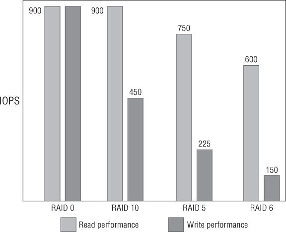
Creating RAID sets not only aggregates the disks' capacity and provides redundancy, but also fundamentally changes their performance characteristics (see Figure 6.2):
Figure 6.2 Performance examples
Interfaces
The interface is the physical connection from the disks. The disks may be connected to a RAID controller in a server, a storage controller, or an enclosure's backplane. Several different types are in use, such as IDE, SATA, SCSI, SAS, and FC, and each has its own standards with different recognized speeds. For example, SATA throughput is 1.5 Gbps, SATA II is backward compatible but qualified for 3 Gbps, and SATA III ups this to 6 Gbps.
Controllers
Controllers sit between the disks and servers, connected via the disk (and enclosure) interfaces on one side and the connectors to the server on the other. Manufacturers may refer to them as controllers, but the terms SPs and heads are often used in SAN hardware. Redundancy is often provided by having two or more controllers in an array.
Controllers are really mini-computers in themselves, running a customized OS. They're responsible for most of the special features available today, such as deduplication, failover, multipathing, snapshots, replication, and so on. Onboard server controllers and SAN controllers present their storage as block storage (raw LUNs), whereas NAS devices present their storage as a usable file system such as NFS. However, the waters become a little murky as vendors build NAS facilities into their SANs and vice versa.
Controllers almost always use an amount of non-volatile memory to cache the data before destaging it to disk. This memory is orders of magnitude faster than disks and can significantly improve IOPS. The cache can be used for writes and reads, although write cache normally has the most significance. Write cache allows the incoming data to be absorbed very quickly and then written to the slower disks in the background. However, the size of the cache limits its usefulness, because it can quickly fill up. At that point, the IOPS are again brought down to the speed of the disks, and the cache needs to wait to write the data out before it can empty itself and be ready for new data.
Controller cache helps to alleviate some of the effect of RAID write penalties mentioned earlier. It can collect large blocks of contiguous data and write them to disk in single operation. The earlier RAID calculations are often changed substantially by controllers; they can have a significant effect on overall performance.
Transport
The term transport in this instance describes how data gets from the servers to the arrays. If you're using a DAS solution, this isn't applicable, because the RAID controller is normally mounted directly to the motherboard. For shared storage, however, a wide variety of technologies (and therefore design decisions) are available. Transport includes the protocol, the topology, and the physical cables/connectors and any switching equipment used. The protocol you select determines the physical aspects, and you can use a dizzying array of methods to get ones and zeros from one rack to another.
Later in the chapter in “Choosing a Protocol,” we'll examine the types of protocols in more depth, because it's an important factor to consider when you're designing a storage architecture. Each protocol has an impact on how to provide the required redundancy, multipathing options, throughput, latency, and so on. But suffice it to say, the potential storage protocols that are used in a vSphere deployment are Fibre Channel (FC), FCoE, iSCSI, and NFS.
Other Performance Factors to Consider
In addition to the standard storage components we've mentioned, you can customize other aspects to improve performance.
Queuing
Although block storage, array controllers, LUNs, and host bus adapters (HBAs) can queue data, there can still be a bottleneck from outstanding I/O. If the array can't handle the level of IOPS, the queue fills faster than it can drain. This queuing causes latency, and excessive amounts can be very detrimental to overall performance. When the queue is full, the array sends I/O-throttling commands back to the host's HBAs to slow down the traffic. The amount of queuing, or queue depth, is usually configurable on devices and can be optimized for your requirements. The QUED column in esxtop shows the queuing levels in real time.
Each LUN gets its own queue, so changes to HBA queue depths can affect multiple LUN queues. If multiple VMs are active on a LUN, you also need to update the Disk.SchedNumReqOutstanding value. This is the level of active disk requests being sent to the LUN by the VMs. Normally, that value should equal the queue-depth number. (VMware's Knowledge Base article 1267 explains how to change these values: http://kb.vmware.com/kb/1267.)
The default queue-depth settings are sufficient for most use cases. However, if you have a small number of very I/O-intensive VMs, you may benefit from increasing the queue depth. Take care before you decide to change these values; it's a complex area where good intentions can lead to bigger performance issues. Increasing queue depth on the hosts unnecessarily can create more latency than needed. Often, a more balanced design, where VM loads are spread evenly across HBAs, SPs, and LUNs, is a better approach than adjusting queue-depth values. You should check the array and the HBA manufacturer's documentation for their recommendations.
Partition Alignment
Aligning disk partitions can make a substantial difference—up to 30 percent in the performance of some operations. When partitions are aligned properly, it increases the likelihood that the SAN controller can write a full stripe. This reduces the RAID write penalty that costs so much in terms of IOPS.
You need to address partition alignment on vSphere in two areas: the VMFS volume and the guest OS file system. When you create VMFS datastores from within the vSphere client, it aligns them automatically for you. In most cases, local VMFS isn't used for performance-sensitive VMs; but if you're planning to use this storage for such tasks, you should create the partition in the client.
The most likely place where partitions aren't aligned properly is in the guest OSes of the VMs. Chapter 7 will have a more in-depth examination of this topic and how to align or realign a VM's partitions.
Workload
Every environment is different, and planning the storage depends on what workloads are being generated. You can optimize storage for different types of storage needs: the ratio of reads to writes, the size of the I/O, and how sequential or random the I/O is.
Writes always take longer than reads. Individual disks are slower to write data than to read them. But more important, the RAID configurations that have some sort of redundancy always penalize writes. As you've seen, some RAID types suffer from write penalties significantly more than others. If you determine that you have a lot of writes in your workloads, you may attempt to offset this with a larger controller cache. If, however, you have a negligible number of writes, you may choose to place more importance on faster disks or allocate more cache to reads.
The size of I/O requests varies. Generally speaking, larger requests are dealt with more quickly than small ones. You may be able to optimize certain RAID settings on the array or use different file-system properties.
Sequential data can be transferred to disk more quickly than random data because the disk heads don't need to move around as much. If you know certain workloads are very random, you can place them on the faster disks. Alternatively, most controller software attempts to derandomize the data before it's destaged from cache, so your results may vary depending on the vendor's ability to perform this efficiently.
VMs
Another extremely important aspect of your design that impacts your storage performance is the VMs. Not only are they the customers for the storage performance, but they also have a role to play in overall speed.
Naturally, this will be discussed in more depth in Chapter 7, but it's worth noting the effect it can have on your storage design. How you configure a VM affects its storage performance but can also affect the other VMs around it. Particularly I/O-intensive VMs can affect other VMs on the same host, datastore (LUN), path, RAID set, or controller. If you need to avoid IOPS contention for a particular VM, you can isolate it, thus guaranteeing it IOPS. Alternatively, if you wish to reduce the impact of I/O from VMs on others, you can spread the heavy hitters around, balancing the load. Chapter 8, “Datacenter Design,” also looks at how disk shares can spread I/O availability.
We've already mentioned guest OS alignment, but you can often tune the guest OS to the environment for your storage array. The VM's hardware and drivers also have an impact on how it utilizes the available storage. How the data is split across VMDKs, whether its swapfile is segregated to a separate VMDK, and how the balance of different SAN drive types and RAIDing are used for different VM disks all affect the overall storage design.
vSphere Storage Performance Enhancements
Later in the chapter, we look at the result of several vSphere technologies that can have an impact on the performance of your VMs. Features such as Storage I/O Control (SIOC), VAAI, and Storage DRS can all improve the VMs' storage performance. Although these don't directly affect the array's performance per se, by optimizing the VMs' use of the array, they provide a more efficient and overall performant system.
Newer Technologies to Increase Effective IOPS
Recently, many SAN vendors have been looking at ways to improve the performance of their arrays. This is becoming important as the density of IOPS required per disk has risen sharply. This jump in the need for IOPS is partly because of the consolidation that vSphere lends itself to, and partly due to advancements in capacity optimizations, such as deduplication.
Write Coalescing
Coalescing is a function of most SPs to improve the effective IOPS. It attempts to take randomized I/O in the write cache and reorganize it quickly into more sequential data. This allows it to be more efficiently striped across the disks and cuts down on write latency. By its very nature, coalescing doesn't help optimize disk reads, so it can only help with certain types of I/O.
Large Cache
Today's controller cache can vary from around 256 MB on a server's RAID controller to hundreds of gigabytes on larger enterprise SANs.
Some SAN vendors have started to sell add-on cards packed with terabytes of nonvolatile memory. These massive cache cards are particularly helpful in situations where the data is being compressed heavily and IOPS/TB are very high. A good example is virtual desktop infrastructure (VDI) workloads such as VMware View deployments.
Another approach is to augment the existing controller cache with one or more flash drives. These aren't as responsive as the onboard memory cache, but they're much less expensive and can still provide speeds that are exponentially (at least 50 times) more than the SAS/SATA disks they're cache for. This relatively economical option means you can add terabytes of cache to SANs.
These very large caches are making massive improvements to storage arrays' IOPS. But these improvements can only be realized in certain circumstances, and it's important that you consider your own workload requirements.
The one criticism of this technique is that it can't preemptively deal with large I/O requests. Large cache needs a period of time to warm up when it's empty, because although you don't want to run out of cache, it isn't very useful if it doesn't hold the data you're requesting. After being emptied, it takes time to fill with suitable requested data. So, for example, even though SP failover shouldn't affect availability of your storage, you may find that performance is heavily degraded for several hours afterward as the cache refills.
Cache Prefetch
Some controllers can attempt to prefetch data in their read caches. They look at the blocks that are being requested and try to anticipate what the next set of blocks might be, so they're ready if a host subsequently requests it. Vendors use various algorithms, and cache prefetch relies on the sort of workloads presented to it. Some read the next set of blocks; others do it based on previous reads. This helps to deliver the data directly from the cache instead of having to wait for slower disks, thus potentially improving response time.
Cache Deduplication
Cache deduplication does something very similar to disk deduplication, in that it takes the contents of the cache's data and removes identical blocks. It effectively increases the cache size and allows more things to be held in cache. Because cache is such a critical performance enhancement, this extra cache undoubtedly helps improve the array's performance. Cache deduplication can be particularly effective when very similar requests for data are being made, such as VDI boot storms or desktop recomposes.
Tiering
Another relatively new innovation on midrange and enterprise SANs is the tiering of disks. Until recently, SANs came with 10 K or 15 K drives. This was the only choice, along with whatever RAIDing you wanted to create, to divide the workload and create different levels of performance. However, SATA disks are used increasingly, because they have large capacity and are much less expensive. Add to that the dramatic drop in prices for flash drives, which although smaller provide insane levels of performance, and you have a real spread of options. All of these can be mixed in different quantities to provide both the capacity and the performance required.
Initially, only manual tiering was available: SAN administrators created disk sets for different workloads. This was similar to what they did with drive speeds and different types of RAID. But now you have a much more flexible set of options with diverse characteristics.
Some storage arrays have the ability to automate this tiering, either at the LUN level or down to the block level. They can monitor the different requests and automatically move the more frequently requested data to the faster flash disks and the less requested to the slower but cheaper SATA disks. You can create rules to ensure that certain VMs are always kept on a certain type of disk, or you can create schedules to be sure VMs that need greater performance at set times are moved into fast areas in advance.
Automatic tiering can be very effective at providing extra IOPS to the VMs that really need it, and only when they need it. Flash disks help to absorb the increase in I/O density caused by capacity-reduction techniques. Flash disks reduce the cost of IOPS, and the SATA disks help bring down the cost of the capacity.
Host-Based Flash Cache
An increasingly popular performance option is host-based caching cards. These are PCIe-based flash storage, which due to the greater throughput available on the PCIe bus are many times faster than SATA- or SAS-based SSD flash drives. At the time of writing, the cards offer hundreds of GBs of storage but are largely read cache. Current market examples of this technology are the Fusion-io cards and EMC's VFCache line.
Host-based flash cache is similar to the large read cache options that are available on many of the mainstream storage arrays, but being host-based the latency is extremely low (measured in microseconds instead of milliseconds). The latency is minimal because once the cache is filled, the requests don't need to traverse the storage network back to the SAN. However, instead of centralizing your large read cache in front of your array, you're dispersing it across multiple servers. This clearly has scalability concerns, so you need to identify the top-tier workloads to run on a high performance cluster of servers. Currently the majority of the PCIe cards sold are only for rack servers; blade-server mezzanine cards aren't generally available, so if an organization is standardizing on blades, it needs to make exceptions to introduce this technology or wait until appropriate cards become available.
Most PCIe flash-based options are focused as read-cache devices. Many offer write-through caching; but because most use nonpersistent storage, it's advisable to only use this write cache for ephemeral data such as OS swap space or temporary files. Even if you trust this for write caching, or the device has nonvolatile storage, it can only ever act as a write buffer to your back-end storage array. This is useful in reducing latency and absorbing peaks but won't help with sustained throughput. Buffered writes eventually need to be drained into the SAN; and if you saturate the write cache, your performance becomes limited by the underlying ingest rate of the storage array.
PCIe flash-based cache is another option in the growing storage tier mix. It has the potential to be very influential if the forthcoming solutions can remain array agnostic. If it's deeply tied to a vendor's own back-end SAN, then it will merely be another tiered option. But if it can be used as a read cache for any array, then this could be a boon for customers who want to add performance at levels normally available only in the biggest, most expensive enterprise arrays. Eventually, PCIe flash read caches are likely to be overtaken by the faster commodity RAM-based software options, but it will be several years before those are large enough to be beneficial for wide-scale uptake. In the meantime, as prices drop, PCIe cards and their driver and integration software will mature, and the write-buffering options will allow them to develop into new market segments.
RAM-Based Storage Cache
A new option for very high I/O requirements is appliances that use server RAM to create a very fast read cache. This is particularly suitable for VDI workloads where the desktop images are relatively small in size, are good candidates for in-cache deduplication, but generate a lot of I/O. The entire desktop image can be cached in RAM (perhaps only 15 GB worth for a Windows 7 image), and all the read requests can be served directly from this tier. This can be a dedicated server for caching or a virtual appliance that grabs a chunk of the ESXi server's RAM. RAM is orders of magnitude faster than local SAS/SATA SSD or even PCIe flash, so performance is extremely impressive and helps to reduce the high IOPS required of the shared storage. Atlantis's ILIO software is an example of such a product.
With vSphere 5.0, VMware introduced a host capability called content based read cache (CBRC) but opted to keep it disabled by default. When VMware View 5.1 was released about six months later, View had a feature called View Storage Accelerator that enabled and utilized the CBRC. CBRC is VMware's answer to RAM-based storage cache. It keeps a deduplicated read cache in the host server's RAM, helping to deliver a faster storage response and absorbing the peaks associated with VDI workloads.
Server memory cache will only ever provide a read-cache option due to the volatile nature of RAM. Read caches for VDI are useful in reducing peaks, particular in boot-storm type scenarios, but VDI is an inherently write-intensive workload. The argument goes that if you're offloading huge chunks of reads, the back-end storage arrays can concentrate on write workloads. VDI is becoming the poster child of read-cache options, because of the relatively small capacity requirements but high IOPS required. Anyone who has tried to recompose hundreds of desktop VMs on an underscaled array knows how painful a lack of horsepower can be.
Although RAM continues to drop in price and grow in capacity, it will always be an expensive GB/$ proposition compared to other local flash-based storage. It will be interesting to see how valuable RAM cache becomes for more generalized server workloads as it becomes feasible to allocate more sizable amounts of RAM as a read-cache option. The ability of centralized storage arrays to deal more efficiently with heavy write loads will become increasingly crucial.
Measuring Your Existing IOPS Usage
When you know what affects the performance of your storage and how you can improve the design to suit your environment, you should be able to measure your current servers and estimate your requirements.
Various tools exist to measure performance:
- Iometer (www.iometer.org/) is an open source tool that can generate different workloads on your storage device. It lets you test your existing storage or generate suitable workloads to test new potential solutions.
- To monitor existing VMs, start with the statistics available in the vSphere client. You can also use esxtop to look at the following statistics:
- DAVG—Disk latency at the array
- KAVG and QUED—Queue-depth statistics showing latency at the VMkernel
- For very in-depth VM monitoring, the vscsiStats tool provides a comprehensive toolset for storage analysis.
- Windows VMs and physical servers can monitor IOPS with the perfmon tool. Just add the counters Disk Reads/sec and Disk Writes/sec from the Physical Disk performance objects to view the IOPS in real time. These can then be captured to a CSV file so you can analyze typical loads over time.
- Linux/Unix VMs and physical servers can use a combination of top and iostat to perform similar recordings of storage usage.
When you're testing VMs, it's worth noting that the hypervisor can create some inaccuracies in guest-based performance tools such as perfmon due to timing issues, especially when the CPU is under strain. Remember to take into account the requirements of nonvirtual servers that may use the same storage, because they may affect the performance of the VMs.
vSphere has added new host and VM performance metrics in both the vSphere Client and in esxtop/resxtop. These additional statistics cover both real-time and trending in vCenter and bring the NFS data on par with the existing block-based support. To make the most of the tools, use the latest host software available.
Local Storage vs. Shared Storage
Shared storage, aka SANs or NAS devices, have become so commonplace in vSphere deployments that local storage is often disregarded as an option. It's certainly true that each new release of VMware's datacenter hypervisor layers on more great functionality that takes advantage of shared storage. But local storage has its place and can offer tangible advantages. Each design is different and needs to be approached with an open mind. Don't dismiss local storage before you identify the real needs of your company.
Local Storage
Local storage, or DAS, can come in several forms. Predominantly, we mean the disks from which you intend to run the VMs, mounted as VMFS datastores. These disks can be physically inside or attached to the host's disk bays. The disks can also be in a separate enclosure connected via a SCSI cable to an external-facing SCSI card's connector. Even if externally mounted, it's logically still local host storage. With local storage, you can mount a reasonable amount of capacity via local SCSI.
You can install vSphere 5 locally on SCSI, SAS, and SATA disks or USB flash drives (including SD cards), although your mileage may vary if the disk controller isn't listed on VMware's approved HCL. Theoretically you can use any of them for local storage for VMs, but clearly USB/SD flash storage was only meant to load the ESXi OS and not to run VMs.
First, let's identify more clearly when you don't want to deploy VMs on local storage. Certain features need storage that multiple hosts can access; if these will be part of your solution, you'll need at least some shared storage. Make no mistake, there are definite advantages to using shared storage (hence its overwhelming popularity):
- Local storage can't take advantage of DRS. Although enhancements in vSphere 5.1 mean that shared storage is no longer a requirement for vMotion, DRS still won't move VMs on local storage.
- High availability (HA) hosts need to be able to see the same VMs to recover them when a protected host fails.
- FT hosts need a second host to access the same VM, so it can step in if the first host fails.
- You can manage storage capacity and performance as a pool of resources across hosts, the same way host clusters can pool compute resources. SIOC, Storage DRS, and Policy-Driven Storage features discussed later in the chapter demonstrate many of the ways that storage can be pooled this way.
- RDM disks can't use local storage. In turn, this excludes the use of Microsoft clustering across multiple hosts.
- When you use shared storage, you can recover from host failures far more easily. If you're using local storage and a server fails for whatever reason, the VMs will be offline until the server can be repaired. This often means time-consuming backup restores. With shared storage, even without the use of HA, you can manually restart the VMs on another cluster host.
- Local storage capacity is limited by several factors, including the size of the SCSI enclosures, the number of SCSI connectors, and the number of datastores. Generally, only so many VMs can be run on a single host. As the number of hosts grows, the administrative overhead soon outweighs the cost savings.
- Performance may also be limited by the number of spindles available in constrained local storage. If performance is an issue, then SSD can be adopted locally, but it's expensive to use in more than a handful of servers and capacity becomes a problem again.
- With shared storage, it's possible to have a common store for templates and ISOs. With local storage, each host needs to have a copy of each template.
- It's possible with shared storage to run ESXi from diskless servers and have them boot from SAN. This effectively makes the hosts stateless, further reducing deployment and administrative overheads.
With all that said, local storage has some advantages of its own. If you have situations where these features or benefits aren't a necessity, then you may find that these positives create an interesting new solution:
- Far and away the greatest advantage of local storage is the potential cost savings. Not only are local disks often cheaper, but an entire shared-storage infrastructure is expensive to purchase and maintain. When a business is considering shared storage for a vSphere setup, this may be the first time it has ventured into the area. The company will have the initial outlay for all the pieces that make up a SAN or NAS solution, will probably have training expenses for staff, and may even need additional staff to maintain the equipment. This incipient cost can be prohibitive for many smaller companies.
- Local storage is usually already in place for the ESXi installable OS. This means there is often local space available for VMFS datastores, or it's relatively trivial to add extra disks to the purchase order for new servers.
- The technical bar for implementing local storage is very low in comparison to the challenges of configuring a new SAN fabric or a NAS device/server.
- Local storage can provide good levels of performance for certain applications. Although the controller cache is likely to be very limited in comparison to modern SANs, latency will be extremely low for obvious reasons.
- You can use local storage to provide VMFS space for templates and ISO files. Using local storage does have an impact. Localized templates and ISOs are available only to that host, which means all VMs need to be built on the designated host and then cold-migrated to the intended host.
- You can also use local storage for VM's swap files. This can save space on the more expensive shared storage for VMs. However, this approach can have an effect on DRS and HA if there isn't enough space on the destination hosts to receive migrated VMs.
- Many of the advanced features that make shared storage such an advantage, such as DRS and HA, aren't available on the more basic licensing terms. In a smaller environment, these licenses and hence the features may not be available anyway.
- Local storage can be ideal in test lab situations, or for running development and staging VMs, where redundancy isn't a key requirement. Many companies aren't willing to pay the additional costs for these VMs if they're considered nonessential or don't have SLAs around their availability.
vSphere 5.1's vMotion enhancements, which allow VMs on local disks to be hot migrated, reaffirm that local VMFS storage can be a valid choice in certain circumstances. Now hosts with only local storage can be patched and have scheduled hardware outages with no downtime using vMotion techniques. Local storage still has significant limitations such as no HA or DRS support, but if the budget is small or the requirements are low then this may still be a potential design option.
What about Local Shared Storage?
Another storage possibility is becoming increasing popular in some environments. There are several different incarnations, but they're often referred to as virtual SANs, virtual NAS, or virtual storage devices. They use storage (normally local) and present it as a logical FC, iSCSI, or NFS storage device. Current marketplace solutions include VMware's own VSA (see sidebar), HP's LeftHand, StarWind Software, and NexentaVSA.
VSA Appliances
VSA Requirements
- Minimum 6 GB of RAM (24 GB is recommended)
- At least four network adapters (no jumbo frames)
VSA Performance
- Speed of the disks
- Number of disks
- RAID type
VSA Appliances
VSA Requirements
- Minimum 6 GB of RAM (24 GB is recommended)
- At least four network adapters (no jumbo frames)
VSA Performance
- Speed of the disks
- Number of disks
- RAID type
- Local RAID controller (the size of the onboard write cache is particularly relevant)
- Speed/quality of the replication network (VSA's internode host-mirrored disk replication is synchronous, which means VM disk writes aren't acknowledged until they're written to both copies)
VSA Design Considerations
- Eight 3 TB disks in RAID 6 with no hot spare. This provides 18 TB of usable space on a two host cluster or 27 TB across three hosts (each datastore must have room to be mirrored once).
- Twenty-eight 2 TB disks in RAID 6 (sixteen of them in an external enclosure in their own RAID 6 group) with no hot spare. This provides 24 TB of usable space on a two host cluster or 36 TB across three hosts.
Virtual arrays allow you to take advantage of many of the benefits of shared-storage devices with increased VMware functionality but without the cost overheads of a full shared-storage environment. Multiple hosts can mount the same LUNs or NFS exports, so the VMs appear on shared storage and can be vMotioned and shared among the hosts. Templates can be seen by all the hosts, even if they're stored locally.
But remember that these solutions normally still suffer from the same single-point-of-failure downsides of local storage. There are products with increasing levels of sophistication that allow you to pool several local-storage sources together and even cluster local LUNs into replica failover copies across multiple locations.
Several storage vendors also produce cut-down versions of their SAN array software installed within virtual appliances, which allow you to use any storage to mimic their paid-for storage devices. These often have restrictions and are principally created so that customers can test and become familiar with a vendor's products. However, they can be very useful for small lab environments, allowing you to save on shared storage but still letting you manage it the same way as your primary storage.
Additionally, it's feasible to use any server storage as shared resources. Most popular OSes can create NFS exports, which can be used for vSphere VMs. In fact, several OSes are designed specifically for this purpose, such as the popular Openfiler project (www.openfiler.com) and the FreeNAS project (http://freenas.org). These sorts of home-grown shared-storage solutions certainly can't be classed as enterprise-grade solutions, but they may give you an extra option for adding shared features when you have no budget. If your plan includes regular local storage, then some virtualized shared storage can enhance your capabilities, often for little or no extra cost.
Shared Storage
Shared storage provides the cornerstone of most vSphere deployments. Local storage is often still found in small setups, where companies are new to the technologies or lack the budget. To take full advantage of vSphere and all it has to offer, a shared-storage solution is the obvious first choice. Shared storage underlines the primary goals:
Choosing a Protocol
An increasingly discussed and debated storage topic is which protocol to use. VMware supports several protocols, and with that choice come decisions. With the advent of 10GbE, network-based iSCSI and NFS have become far more competitive against FC-based SANs. Many of the midrange arrays available today come with multiple protocol support included or easily added, so things are much less clear cut than before.
As you'll see, each protocol has its own ups and downs, but each is capable and should be considered carefully. Old assumptions about the protocols can and should be questioned, and preconceptions are often being proven no longer true. It really is time to go back to the requirements and ask why.
As each new release of vSphere becomes available, the support matrix for protocols changes; and the maximum configuration limits regularly increase. In past VMware days, many advanced features or products only worked with certain types of storage. For the most part, this is no longer true: most products work with all supported protocols.
You need to compare the following protocols: FC, iSCSI (using both hardware and software initiators), and NFS exports. A newer addition to the list is Fibre Channel over Ethernet (FCoE); and you should also consider the increasing availability of 10GbE, which is making a big impact on the storage landscape with regard to protocol selection. A few other options are available on the vSphere protocol list, but they're excluded from the rest of this discussion because they aren't considered sufficiently mainstream to be relevant to most readers. These additional options are either vendor specific or used in very specific use cases:
For the rest of this chapter, we'll concentrate on the four most common protocols. These are the protocols for which you can expect hardware vendors to provide solutions and that you'll encounter in vSphere environments. Table 6.3 and Table 6.4 summarize the characteristics of each protocol.
Table 6.3 Protocol hardware characteristics
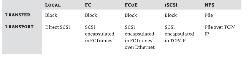
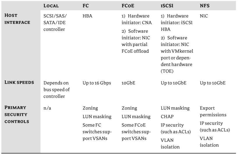
Table 6.4 vSphere feature comparison for each protocol
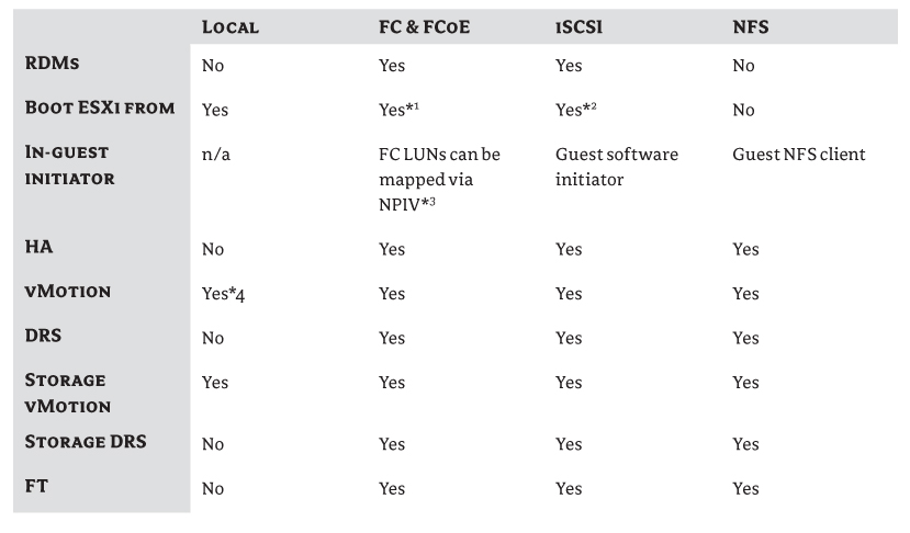
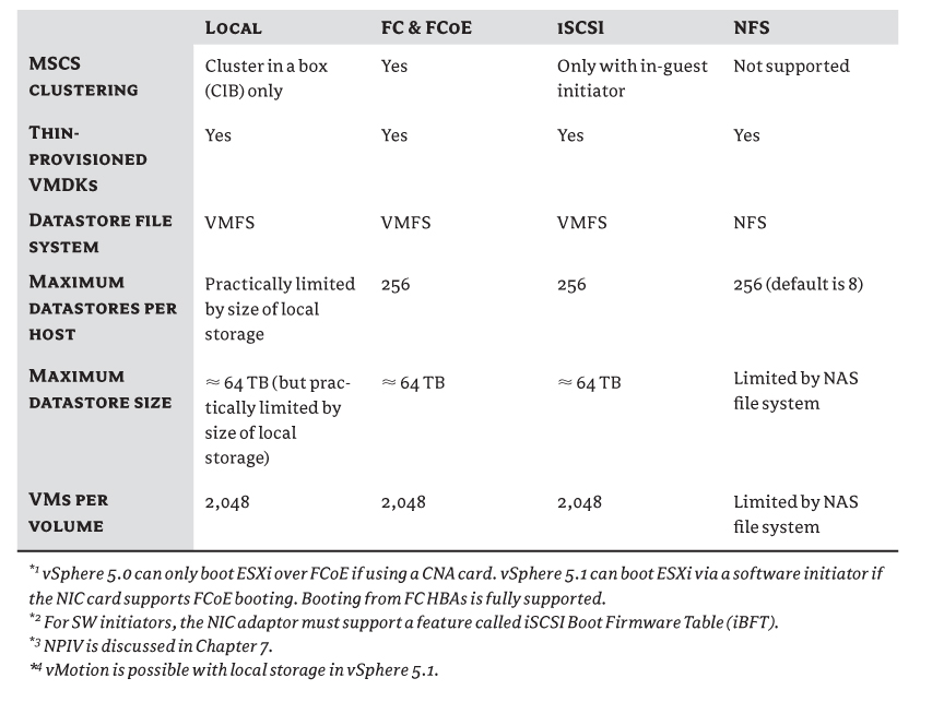
Fibre Channel
FC is the veritable stalwart shared-storage protocol and has been ever since it was first supported by ESX in version 2.0. It's a mature and well-trusted solution in datacenters, and traditionally it's the default solution of many Enterprise SANs. The FC protocol encapsulates all the SCSI commands into FC frames, a lossless transport.
FC fabrics are specialized storage networks made up of server HBAs, FC switches, and SAN SPs. Each connector has a globally unique identifier known as a World Wide Name (WWN). A WWN is further split into a World Wide Port Name (WWPN), which is an individual port, and a World Wide Node Name (WWNN), which is an endpoint device. Ergo, a dual-port HBA will have two WWPNs but only one WWNN.
Hosts can be attached directly to the SAN without the use of a fabric switch, but this restricts the number of hosts to the number of FC SP ports available. FC switches also allow for redundant links from each host to cross-connect to multiple SP controllers.
The FC protocol is a high-bandwidth transport layer with a very low latency. This low latency still sets it apart from other common storage protocols. The FC protocol technically has three different modes, but switched (FC-SW) is the only one you're likely to use in a vSphere environment (point-to-point and arbitrated loop are the two legacy modes). The interconnect speeds are set at 1, 2, 4, 8, or the latest, 16 Gbps. vSphere 5.0 requires that 16 Gbps HBAs be throttled back to 8 Gbps, but vSphere 5.1 supports 16Gbps to the FC switch. To get full 16Gbps to the array, multiple 8Gbps connections from the FC switch to the array need added to the zone. FC fabrics ordinarily use OM2 cables with LC connectors (orange fiber optic cables) these days, although light-blue OM3 cables are becoming more popular with an increase in 8 and 16 Gbps use.
FC storage security is predominantly handled via zoning. Zoning is an access-control mechanism set at the FC switch level, restricting which endpoints can communicate. Anything outside the zone isn't visible to the endpoint. Zoning protects devices from other traffic such as registered state-change notification (RSCN) broadcasts and is roughly analogous to VLANing in the Ethernet world. Zoning ensures that hosts that need to see the storage can do so, while those that don't need visibility don't interfere. You can set zones based on specific switch ports (port zoning or hard zoning) or define them via WWNs (soft zoning), which has the advantage of allowing recabling without needing to reconfigure the zoning information. Due to security concerns, some FC switch manufacturers only support hard zoning on their newer switches.
Several zoning topologies are available. The simplest method is to have one large zone with all devices in it. But for vSphere (and most other applications), the recommendation is to use what is called single initiator zoning. This means each HBA is in its own zone with the target device. This approach is considerably more secure and prevents initiators from trying to communicate with each other (which they shouldn't be doing in a vSphere setting). An even tighter convention, known as single initiator/single target zoning, is to create zones so each single HBA is mapped to a single SP. This takes longer to configure than the other two zoning topology designs; but if you use a sensible naming convention for the zones (for example, HOSTNAME_HBA1_SPA), they can be logical to follow and you can add to them when required.
You can use LUN masking to grant permissions, allowing LUNs to be available to hosts. The LUN masks are set on the hosts themselves or on the SPs. LUN masking is also sometimes referred to as iGroups, access control, storage presentation, or partitioning. It effectively gives hosts the ability to disregard LUNs or lets SPs ignore hosts that shouldn't be accessing LUNs.
FC has many advantages when compared to other options:
But there are certain potential drawbacks to the FC protocol:
Fibre Channel over Ethernet
FCoE is a relatively new addition to the protocol list available to vSphere architects. FCoE maps the frame-based FC protocol over Ethernet alongside its IP traffic. Because Ethernet has no built-in flow control, FC needs special enhancements to prevent congestion and packet loss. These enhancements help to deal with the loss and retransmissions in IP-based transport, which is what makes FCoE special. FCoE is designed to run over 10GbE cables.
FCoE can utilize converged network adapters (CNAs), which combine FC HBAs and Ethernet NIC adapters. ESXi often need extra drivers installed for these CNA cards to be recognized. The drivers usually come in two parts: one for the FCoE piece and another for the Ethernet adapter. After the card is installed, it logically appears in the vSphere Client as both an HBA under the storage adapter configuration and as a NIC under the network adapter configuration.
Since vSphere 5.0, the hypervisor offers a software initiator that works with 10GbE NIC cards that include a partial FCoE offload capability. This allows you to access LUNs over FCoE without needing a CNA card or installing third-party CNA drivers. To create the FCoE software adapter on the ESXi host, enable the feature on the NIC adapter. The NIC must be an uplink on a vSwitch that already contains a VMkernel connection. It uses the VMkernel to negotiate the FCoE connection with the physical switch. This connection isn't used for FCoE storage traffic. vSphere 5.0 can boot from a SAN LUN on FCoE if you have a FCoE hardware initiator HBA card, but 5.1 added the ability to boot from FCoE software initiator if the NIC card supports FCoE booting.
FCoE has a great deal of overlap with FC, so if you have an existing FC infrastructure, you should be able to introduce FCoE while avoiding a rip-and-replace style of migration. FCoE is partially important in converged 10GbE infrastructures, such as Cisco's UCS blades, where there is no FC connection to the servers. All traffic, including storage, leave the servers and traverse an Ethernet network initially. In such converged solutions, the physical transport may be fiber or copper based to the northbound switch but is always Ethernet not FC based. To provide connectivity to FC storage arrays, the FC fabric switches cross-connect to the network switches. The FCoE-capable network switches can then relay the FCoE traffic into the FC fabric. If newer SANs have 10GbE connections and can natively use the FCoE protocol, then they can connect directly to the FCoE-capable network switches, which act solely as the fabric with no need for FC switches in the design.
FCoE uses the same zoning techniques as the FC world to regulate access between FCIDs (equivalent of FC WWPNs). FCoE requires Jumbo Frames because the payloads are larger than 1,500 bytes and can't be fragmented.
FCoE shares many of the advantages attributed to FC, along with the following:
But be mindful of these potential FCoE disadvantages:
iSCSI
iSCSI uses TCP to encapsulate SCSI traffic, allowing block-level storage LUN access across Ethernet cables. Commonly used over 1GbE links, iSCSI has been able to take advantage of 10GbE advances, letting it compete with the traditionally more performant FC protocol.
iSCSI became popular in datacenters predominantly through use by Microsoft servers (as opposed to FC, which was traditionally the focus of Unix servers).
vSphere supports two types of iSCSI initiator:
The hardware initiators have the advantage that they offload some of the CPU processing; but with recent advances in the vSphere software initiator, this has become less of an issue. The current software initiator uses very little CPU (around half a core); and with the increasing processing power of servers, it's generally thought that the additional cost of the hardware cards is no longer worth the expense. Software initiators have become a much more popular method of connecting to iSCSI targets. Few choose to buy hardware cards for new deployments. Hardware initiators are relatively rare and are used less and less these days.
Although it's possible to run an in-guest iSCSI software initiator to access raw block storage for a VM, it bypasses the ESXi host's storage stack and so is treated like any other VM network traffic. It's unusual for VM traffic to be a bottleneck, but this is the sort of configuration that can saturate VMNICs. This isn't a recommended way to present storage to VMs: it doesn't have the flexibility of regular iSCSI storage, because it can't use Storage vMotion or vSphere snapshots.
vSphere has two methods to discover iSCSI targets:
iSCSI has no FC fabric zoning, although because it's still block-level storage it can use LUN masking to ignore LUNs. Instead of zoning, iSCSI uses Challenge-Handshake Authentication Protocol (CHAP) as a way to provide rudimentary access control for the initiators and targets. CHAP is a three-way handshake algorithm based on a predefined private value, which verifies identity using a hashed transmission. Hardware initiators only allow for the use of one-way CHAP, as opposed to software initiators, which can do mutual CHAP (bidirectional).
Most arrays also let you configure access control based on IP address or initiator name. Make sure your iSCSI traffic is only allowed onto an internal part of your trusted network, because the traffic isn't encrypted in any way. A nonroutable VLAN on a dedicated pair of redundant switches is ideal to segregate and secure iSCSI traffic.
Jumbo frames can be enabled on vSphere hosts and are supported by most iSCSI SANs. They help to increase performance, because the larger packet sizes reduce the overhead of processing the Ethernet packets. Typically, the frames are set to 9,000 maximum transmission units (MTUs). It's important that if you enable jumbo frames, all devices, endpoints (servers and storage), and network devices in between must support and be enabled for this. Enabling jumbo frames on some Cisco switches requires them to be reloaded (which causes a short network outage).
The Ethernet switch ports used for the storage network should have Rapid Spanning Tree Protocol (RSTP) or portfast enabled. This allows an immediate transition if an active link fails.
Chapter 5, “Designing Your Network,” discussed various methods to provide suitable network redundancy for Ethernet-based storage. Later in this chapter, the “Multipathing” section will discuss different multipathing techniques, including those covering the iSCSI protocol. But it's worth pointing out at this juncture that your iSCSI design should carefully consider redundancy. The fundamentals involve ensuring that at least two NICs (or HBAs) are configured on each host for iSCSI traffic. These two NICs should be connected to two separate switches, which in turn are connected to two iSCSI controllers on the SAN.
Dedicated storage switches, which don't handle regular network traffic, make your storage transport more secure. They also help to prevent contention with other IP traffic, improving storage performance. If you don't have access to separate hardware, then you can use layer 2 VLANs to isolate the storage. You should avoid 100 Mbps equipment anywhere in the chain, because it doesn't provide the throughput required to run VMs effectively. Use 1GbE capable switches, NICs, and cables throughout as a minimum.
Ethernet isn't designed for storage, so it can suffer from congestion issues when numerous hosts are attached to a much smaller number of array controllers. This causes oversubscription, which means that packets get dropped and performance degrades. This can be the start of a vicious circle where TCP/IP needs time to see what was dropped and then more time to retransmit. A bad situation gets progressively worse. Using logical separation techniques such as VLANing doesn't help in these cases. If this becomes an issue, you should use dedicated storage switches and, if required, more capable switches with better backplane I/O capacity, which will alleviate the oversubscription.
iSCSI has a number of advantages over the FC and FCoE protocols:
However, you must also remember a number of disadvantages when considering iSCSI:
NFS
NFS is a very mature file-sharing protocol that allows several clients to connect at the same time. NFS file shares are known as exports. vSphere requires that NFS exports use version 3 of the protocol, even though version 4 has been available and ratified for many years.
NFS is fundamentally different from FC, FCoE, and iSCSI in that it isn't block-level storage, but file-level. It's common to refer to the block-level arrays as SAN devices, but refer to NFS as NAS devices, even though many SANs can now provide NFS exports. Block devices provision their disks as LUNs, which can be used as VMFS volumes or RDMs in vSphere. But NFS exports are used as a remote file system, and VMs are placed directly on them.
Traditionally, block storage (particularly FC) had better support for all the latest features. But these days, almost all premier features are available for NFS. In fact, some newer VMware View options have been released for NFS before their block-based alternatives.
NFS has historically been criticized for its performance versus FC and iSCSI. This was due in large part to cheaper NAS devices not being able to stand up against enterprise-class SANs, rather than to a deficiency in the protocol itself. For the vast majority of workloads, NFS is more than capable; and coupled with 10GbE, performance can be comparable to FC 8 Gbps.
Bandwidth is closely related to the physical transport, and there isn't much difference between 8 Gbps FC and 10GbE NFS. IOPS tends to come down to cache and disk spindles/speed, so even 16 Gbps FC connections might not necessarily provide much better performance than 10GbE NFS (or iSCSI or FCoE, for that matter). The primary differences between FC and NFS are latency, failover times, and multipathing mechanisms.
NFS is easy to plan and configure, and it's normally far less costly than FC to set up and maintain. For this reason, it's very popular for small to medium companies and is often the default choice for VDI deployments.
By default, the number of NFS exports that any host can mount is only 8, but an advanced setting allows you to increase this to 256. Even if you think you'll never grow beyond the eight-datastore limit, it's a good idea to increase this number before provisioning the first storage, because an increase in the future requires host reboots.
NFS exports can be mounted on hosts via IP addresses or hostname, but IP address is the recommended choice. If local procedures require you to use hostnames, check to see whether the name servers are virtual. If so, it's advisable to either make an exception and use IP addresses when mounting them, or create entries in the /etc/hosts file of each host. Otherwise, it's possible to get stuck in a chicken-and-egg situation where the hosts can't resolve the NFS exports, because all the name servers are turned off (because they live on the NFS exports). Name resolution is so important to other services that you should plan carefully if all DNS (or WINS) servers are virtual.
As with iSCSI, the network traffic isn't encrypted. And NFS doesn't use CHAP to authenticate initiators and targets, so it's even more important to only span a trusted network. Most NAS devices can isolate their traffic to specific IP hosts, but this is easy to spoof if the network isn't suitably isolated. Unfortunately, the vSphere hosts must mount the exports with root access, which is a security concern in itself. For this reason, dedicated isolated storage switches are highly recommended if security is an especially important design consideration.
You can adjust a number of advanced NFS settings to fine-tune the hosts to the particular NAS unit you're using. You should consult the storage vendor's documentation to ensure that you implement its best practices.
Much of the advice given in the previous section for iSCSI network configurations is just as applicable to NFS. If possible, do the following:
- Separate network devices to isolate the storage traffic.
- Use nonroutable VLANs.
- Use redundant network links.
- Use jumbo frames.
- Enable RSTP or portfast on the switch ports.
- Use switches with sufficient port buffers.
NFS can offer the following advantages (again, many are common with iSCSI because they share the same physical transport layer):
And here are some NFS-specific advantages:
NFS has the following disadvantages in common with iSCSI:
And these are NFS-specific limitations:
- Can't aggregate bandwidth across multiple Ethernet cables (see the “Multipathing” section).
- Not ideally suited to very high I/O VMs that would normally get dedicated datastores/LUNs.
- Uses some additional CPU processing.
- No boot from SAN; you can't boot from an NFS export.
- NFS is particularly susceptible to oversubscription because of the very high VM density possible on each datastore.
Protocol Choice
After carefully looking at the protocols, their constraints, and their impacts, a number of key factors tend to decide which is best suited to a design.
Companies always favor sticking to an existing implementation, and for good reason. You're likely to already have several pieces, and you probably want to avoid a complete rip-and-replace strategy. The ability to carefully transition to a new protocol, especially regarding something as critical as primary storage, is an important consideration. If this is a trusted proven solution that you're merely hoping to upgrade, then existing skills and experience are tangible assets.
Performance is a factor that may influence your decision. In most general situations, FC or 10GbE with iSCSI or NFS is likely to be more than sufficient for 99 percent of your bandwidth needs. The VMs' IOPS come down to several things, but ultimately it's the SP cache, any SP “secret sauce” such as efficient write coalescing, and the number and speed of the underlying disks. The protocol has very little impact in a properly designed environment. However, one key area where performance may influence the protocol choice is latency. If the design requires the potential for very-low-latency VMs (perhaps a real-time database), then FC is your friend (unless you can deal with the limitations of DAS).
NFS grew to be a popular Ethernet alternative to iSCSI during the vSphere 3 and 4 releases because of the larger datastores possible (iSCSI datastores were limited to 2 TB) and SCSI locking issues that could restrict the number of VMs on its datastores. NFS proved to be far more flexible, allowing for large commodity datastores. With vSphere's VMFS-5 datastores up to a maximum of 64 TB, its new ATS locking allowing greater density on iSCSI LUNS, and simplified iSCSI port binding, we think iSCSI is likely to see a resurgence in popularity. iSCSI's significantly better multipathing support provides a serious advantage over NFSv3 in larger environments. Additionally, monitoring and troubleshooting iSCSI as a block-based protocol is arguably better supported on vSphere than NFS. The ease of administering a file-based array will always appeal to the SMB market, whereas larger organizations are better suited to the moderately more complex iSCSI.
Costs can influence the protocol used. Often, NAS devices are cheaper than SANs, and iSCSI SANs are cheaper than FC ones. But many of the latest midrange storage offerings give you the flexibility to pick and mix several of the protocols (if not all of them). FC has always been regarded as the more expensive option, because it uses its own dedicated switches and cables; but if you're trying to compare FC to protocols using 10GbE, and you need new hardware, then both are comparatively priced.
10GbE has the added advantage of potential cable consolidation with your host's networking needs. A 10GbE NIC with partial FCoE offloading is arguably the best of all worlds, because it gives you the greatest flexibility. They can connect to a FC fabric, can provide access to iSCSI or NFS, and act as the host's networking NICs. FCoE CNA hardware is still in a state of flux; and as we've seen with the demise of iSCSI HBAs, now that FCoE software initiators are available in vSphere, the CNA cards are likely to be used less and less. Cisco is pushing forward with its Twinax cables with SPF+ connectors, which have so far become the de facto standard; and Intel is pushing 10GbE-capable adapters onto server motherboards.
An interesting design that's becoming increasingly popular is to not plump for a single protocol, but use several. Most arrays can handle FC and Ethernet connections; so some companies are using NFS for general VM usage with their large datastores, for more flexibility for growth and array-based utilities; and then presenting LUNs on the same storage via FC or iSCSI for the VMs more sensitive to I/O demands. It's the ultimate multipathing option.
Finally, remember that DAS can be a viable option in certain, albeit limited circumstances. If you're deploying a single host in a site, such as a branch office, then introducing an additional storage device only introduces another single point of failure. In that situation, shared storage would be more expensive, would probably be less performant, and would offer no extra redundancy.
Multipathing
vSphere hosts use their HBAs/NICs, potentially through fabric switches, to connect to the storage array's SP ports. By using multiple devices for redundancy, more than one path is created to the LUNs. The hosts use a technique called multipathing to make the path-selection decisions.
Multipathing can use redundant paths to provide several features such as load balancing, path management (failover), and aggregated bandwidth. Unfortunately, natively vSphere only allows a single datastore to use a single path for active I/O at any one time, so you can't aggregate bandwidth across links.
SAN Multipathing
VMware categorize SANs into two groups:
vSphere hosts by default can use only one path per I/O, regardless of available active paths. With active/active arrays, you pick the active path to use on a LUN-by-LUN basis (fixed). For active/passive arrays, the hosts discover the active path themselves (MRU).
Native Multipathing Plugin
vSphere 4 introduced a redesigned storage layer. VMware called this its Pluggable Storage Architecture (PSA); and along with a preponderance of Three Letter Acronyms, gave vSphere hosts the ability to use third-party multipathing software—Multipathing Plugins (MPPs).
Without any third-party solutions, hosts use what is called the Native Multipathing Plugin (NMP). The terminology isn't that important, but the NMP's capabilities are, because they dictate the multipathing functionality for the vSphere hosts. To further categorize what native multipathing can do, VMware split it into two separate modules:
SATP
The host identifies the type of array and associates the SATP based on its make and model. The array's details are checked against the host's /etc/vmware/esx.conf file, which lists all the HCL-certified storage arrays. This dictates whether the array is classified as active/active or active/passive. It uses this information for each array and sets the pathing policy for each LUN.
PSP
The native PSP has three types of pathing policies. The policy is automatically selected on a per-LUN basis based on the SATP. However, as you can see in Figure 6.3, you can override this setting manually:
Figure 6.3 Path Selection drop-down
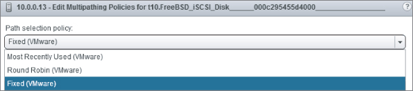
Multipathing Plugin
Array manufacturers can provide extra software plug-ins to install on ESXi hosts to augment the NMP algorithms provided by VMware. This software can then optimize load-balancing and failover for that particular device. This should allow for greater performance because the paths are used more effectively, and potentially enable quicker failover times. EMC and Dell are examples of storage vendors that have a MPP available.
ALUA
Asymmetric arrays can process I/O requests via both controllers at the same time, but each individual LUN is owned/managed by a particular controller. If I/O is received for a LUN via a controller other than its managing controller, the traffic is proxied to it. This proxying adds additional load on the controllers and can increase latency.
Asymmetric logical unit access (ALUA), part of the SPC-3 standard from 2005, is the technology that enables an array to use the controllers' interconnects to service I/O. When the link is used, performance is degraded (asymmetric), and therefore without the use of the appropriate ALUA SATP plugin, vSphere treats it as an active/passive array. When a host is connected to an ALUA-capable array, the array can take advantage of the host knowing it has multiple SPs and which paths are direct. This allows the hosts to make better failover and load-balancing decisions. ALUA also helps to prevent the classic path-thrashing problem that is possible with active/passive arrays.
Both RR and MRU policies are ALUA aware and will attempt to schedule I/O via the LUN's Active-Optimized path. RR is considered a better choice for most Active/Passive arrays, although not all arrays support or recommend this pathing policy so check with your vendor. There are two ALUA transition modes that an array can advertise:
An ALUA array can use either or both modes. vSphere supports all combinations of modes. The controllers' ports are treated collectively via a target portal group (TPG). The TPG advertises the following possible active states to the hosts:
- Active Optimized
- Active Non-Optimized
- Standby
- Unavailable
- In Transition
Paths can be given a ranking via an esxcli command that give administrators some control over the pathing decisions. However, active optimized paths are always picked over active nonoptimized paths, even if their set rank is lower.
VMware licenses the ability to use both third-party MPPs and ALUA. To use either of these functions, you need to purchase vSphere Enterprise licenses.
Additional iSCSI Considerations
iSCSI has some additional SAN multipathing requirements that differ depending on the type of initiator used.
Hardware iSCSI Initiators
When you're using hardware initiators for iSCSI arrays, vSphere multipathing works effectively the same as it does for FC connections. The hosts recognize the HBAs as storage adapters and use the NMP with SATP selection and PSP pathing.
Some iSCSI arrays use only one target, which switches to an alternate portal during failover. Hosts detect only one path in these instances.
Software iSCSI Initiators
Software iSCSI initiators require additional configuration steps to use vSphere's storage MPIO stack. By default, software iSCSI uses the multipathing capabilities of the IP network. The host can use NIC teaming to provide failover, but the initiator presents a single endpoint so no load-balancing is available.
To use the vSphere storage NMP and enable load-balancing across NICs, you must use a technique known as port binding. Don't use network link aggregation, because you want to define separate end-to-end paths. Follow these steps to enable port-binding for two NICs for iSCSI:
Figure 6.4 iSCSI multipathing vSwitch
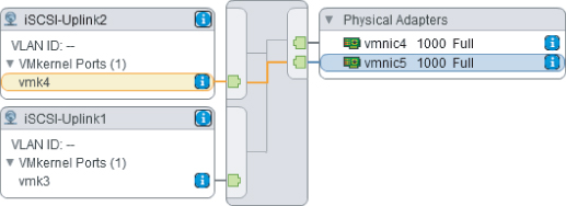
Figure 6.5 iSCSI multipathing port binding
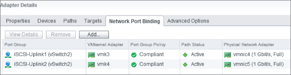
NAS Multipathing
NAS multipathing is fundamentally different than SAN multipathing in vSphere because it relies entirely on the networking stack. MPIO storage tools such as SATPs and PSP aren't available, so IP-based redundancy and routing is used.
For each NFS export mounted by the host, only one physical NIC is used for traffic, despite any link-aggregation techniques used to connect multiple NICs together. NIC teaming provides failover redundancy but can't load-balance an export. But by creating multiple exports along with multiple connections on different subnets, you can statically load-spread datastore traffic.
Chapter 5 looked at designs to provide network redundancy. As an outline, you can use two different methods to create NIC failover for an NFS mount:
- Create two (or more) vSwitches, each with a VMkernel interface, or a single vSwitch with multiple VMkernel uplinks. Each uplink connects to a separate redundant physical switch. The VMkernel interfaces and NFS interfaces are split across different subnets.
- With physical switches that can cross-stack, you need only one VMkernel interface (and so only one IP address). The NAS device still needs multiple IP address targets. The vSwitch needs at least two NICs, which are split across the two cross-stacked switches. The VMkernel's vSwitch has its load-balancing NIC teaming policy set to “Route based on IP hash.” You need to aggregate the physical switch ports into an 802.3ad EtherChannel in static mode, or if you are using a v5.1 vDS you can use its dynamic Link Aggregation Control Protocol [LACP] support to configure the EtherChannel. The vDS 5.1 dynamic LACP support is only for the link aggregation setup, it doesn't change the way the actual network load balancing is done — this is still the IP hash algorithm. vSphere 5.0 introduced a very basic method to load spread. By mounting multiple NFS exports on multiple hosts via FQDNs instead of IP addresses, you can use round-robin DNS to mount the targets under different IP addresses.
The load-based teaming (LBT) algorithm available with the Enterprise Plus license is one technology that can load-balance saturated links if there are multiple VMkernel connections to each uplink, split across multiple subnets pointing to multiple target IPs.
NFS can densely pack VMs onto a single connection point with its large datastores, native thin-provisioning, and NAS-based file locking. Sharing the load across several NICs is particularly important when you're using 1GbE NICs as opposed to 10GbE connections.
It's difficult to achieve good load balancing with NFS datastores, and in practice NFS multipathing tends to be limited to failover. As an environment scales up, load-balancing becomes a more important consideration, and often iSCSI may prove to be more suitable if your array supports it.
Finally, give special consideration to the longer timeouts associated with NFS. FC and even iSCSI fail over much more quickly, but NFS can take long enough that you should adjust the VM's guest OSes to prepare them for the possibility that their disk may be unresponsive for a longer time.
vSphere Storage Features
vSphere version 5 was known as the storage release for good reason. The number of enhancements, performance improvements, and added functionality meant that storage became a first-class citizen in vSphere resource management. Many of the things that administrators have become accustomed to for host management, such as shares, limits, DRS, vMotion, and affinity rules, have storage equivalents now.
Closer communications between vCenter and storage arrays allow much of the heavy lifting to be accomplished by the storage, reducing host involvement. The storage arrays are highly efficient at moving data between disks, so offloading storage tasks helps to improve overall operational efficacy.
More information is being accepted back into vCenter from the arrays. vCenter collates and presents the information in terms of datastores and VMs, allowing administrators to make more informed decisions about VM placement and create policy-based rules to manage the storage.
vSphere Storage APIs
As vSphere has matured as a product, VMware has deliberately focused on creating a great set of partner accessible application programming interfaces (APIs). These APIs provide a consistent experience to write supporting applications and tools against vSphere. APIs are the common methods to interact with vSphere, and they expose features to external developers. They help to ensure that between version upgrades of vSphere, minimal changes are necessary to keep associated applications compatible.
As new features are added to vSphere, APIs are introduced or existing ones augmented to reveal the new functions and create a common way of executing against them. Therefore, software and hardware vendors often have to update their applications and firmware to take advantage of the new features.
Several sets of important storage-related APIs are available. You should check with your vendors to see whether their products support the latest vSphere 5 APIs and if you need to update anything to take advantage of improved compatibility or functionality:
VAAI
vSphere API for Array Integration (VAAI) is a set of storage APIs that VMware initially introduced in vSphere 4.1. These VAAI capabilities are classified into what VMware terms primitives. To use the primitives, the storage array must include appropriate support, and each array may only provide a subset of support with some of the primitives. NFS support wasn't available with the 4.1 release, but 5.0 included some equivalent matching features.
VAAI integration with an array means you can offload storage tasks that are normally performed by the host directly to the array. Doing so reduces host CPU, memory, network, and fabric loads and performs operations more efficiently and quickly. VAAI support is divided between block storage and file storage. Because the underlying storage is different, the implementation of these optimizations differs. Many of the primitives are comparable, but they're treated separately because in practice they're executed differently.
VAAI for Block-Based Datastores
VAAI has the following primitives for block-based datastores:
vmkfstools -y
VAAI for File-Based Datastores (NFS)
vSphere 5.0 added the NFS VAAI equivalents. Vendor-specific vCenter plugins are required for the NFS VAAI primitives:
Use of VAAI is license dependent, so the hosts must have a minimum of an Enterprise-level license to take advantage of the hardware acceleration. The primitives help to remove bottlenecks and offload storage tasks that are expensive for the hosts to perform. This not only improves host efficiency, but also increases scalability and performance.
Check the VMware storage HCL for compatibility with different arrays: some arrays may require a firmware upgrade to support the VAAI primitives, and only a subset of primitives may be available.
VASA
VASA is the set of standardized API connections that provide vCenter with insight into the capabilities of a storage array. If the array supports the API, then it can advertise three primary information sets:
For vCenter to support the array, two things are normally required. First, the array must support the API. Often this means a firmware upgrade to the SPs to add support. VMware's HCL has details on which arrays support VASA and their required array software level. Second, the array vendor will provide a plugin for vCenter or additional software that needs to be installed. This allows vCenter to correctly interpret the data being provided by the array. The information provided may differ between storage vendors.
VASA helps in the planning, configuration, and troubleshooting of vSphere storage. It should reduce the burden normally associated with managing SANs and lessen the number of spreadsheets needed to keep track of LUNs. As you'll see later in this chapter, the administration of several vSphere tools such as profile-driven storage and datastore clusters can benefit from the additional visibility that VASA information can provide. Storage tasks can become more automated, and users have an increased situational awareness with on-hand insight to the array.
Performance and Capacity
Several vSphere storage features are centered around maximizing the performance and capacity of vSphere's storage. Many of the technologies layer on top of each other, resulting in Storage DRS. Others push the limits of the file system or bring some of the innovation found in the storage arrays to use in vCenter operations.
VMFS-5
As of vSphere 5.0, the default VMFS volumes created are VMFS-5. VMFS-3 datastores created by legacy hosts are still supported and fully functional under vSphere 5. A number of enhancements in VMFS-5 provides additional opportunities from a design perspective:
- VMFS-5 datastores can be up to 64 TB in size without having to combine multiple 2 TB LUNs. This reduces the management overhead previously associated with such large datastores. (The extents feature is still available to concatenate additional LUNs, if you need to grow existing volumes with extra space.)
- Very large volumes and file sizes are now possible with 64 TB physical RDMs. VMDKs and virtual RDMs are still limited to 2 TB minus 512 KB.
- A single 1 MB block size is used for all newly created VMFS-5 volumes. These 1 MB block volumes no longer restrict the file size.
- Numerous performance and scalability improvements have been made, such as ATS file locking, an improved subblock mechanism, and small file support. These are perhaps not immediately relevant to design per se, but the functionality they provide, such as expanding the number of VMs per datastore, is important.
- The old variable block sizes are carried over. This can affect the performance of subsequent Storage vMotions.
- An upgraded VMFS-5 volume doesn't have all the scalability enhancements found in native VMFS-5 datastores.
- There may be inconsistencies across your datastores. In addition to the potentially different block sizes, the starting sectors will be different, and datastores under 2 TB will have MBR partitioning (as opposed to GUID partitioning on native VMFS-5).
Storage I/O Control
Storage I/O Control (SIOC) is a feature that was introduced in vSphere 4.1 to improve the spread of I/O from VMs across a datastore. It provides a degree of quality of service by enforcing I/O shares and limits regardless of which host is accessing them. SIOC works by monitoring latency statistics for a datastore; when a predetermined level is reached, SIOC scales back I/O via allotted shares. This prevents any one VM from saturating the I/O channel and allows other VMs on the datastore their fair share of throughput.
Just as CPU and memory shares only apply during contention, SIOC will only balance the I/O spread when the latency figures rise above the predefined levels. SIOC can enforce I/O with set IOPS limits for each VM disk and distributes load depending on the datastore's total shares. Each host with VMs on the datastore uses an I/O queue slot relative to the VM's shares, which ensures that high-priority VMs receive greater throughput than lower-priority ones.
In vSphere 5.0, this feature has been extended to NFS datastores (previously only VMFS volumes were supported). RDM disks still aren't supported.
To configure SIOC, do the following:
By just enabling SIOC on the datastore, you're automatically protecting all the VMs from a VM that is trying to hog the I/O to a datastore. Without any adjustment in the second step, all the disks will be treated equally; so unless you need to prioritize particular VMs, enabling it on each datastore is all that's required. If you're worried about a specific VM being a bully and stealing excessive I/O, then a limit on that one VM is all that's required. However, just as with CPU and memory limits, be careful when applying limits here because they artificially block the performance of the VM's disks and apply even when there is no contention on that datastore's I/O. Shares are the fairest method to use and the least likely to cause unexpected side effects.
SIOC only works if it knows about all the workloads on a particular datastore. If the underlying disk spindles are also assigned to other LUNs, then SIOC will have problems protecting and balancing I/O for the VMs, and a vCenter alarm will trigger. You should set the same share values across any datastores that use the same underlying storage resources. SIOC requires an Enterprise Plus license for every host that has the datastore mounted.
It's possible to adjust the threshold value set on each datastore. By default in vSphere 5.0, it's set to 30 ms, but you can use any value from 10 ms up to 100 ms. The default value is appropriate in most circumstances; but if you want to fine-tune it to a specific disk type, then SSD datastores can be set lower at around 10–15 ms, FC and SAS disks at 20–30 ms, and SATA disks at 30–50 ms. Setting the value too high reduces the likelihood that SIOC will kick in to adjust the I/O queues. Setting it too low means shares are enforced more frequently, which can unnecessarily create a negative impact on the VMs with lower shares. vSphere 5.1 automatically determines the best latency threshold value to use for each datastore. It tests the datastore's maximum throughput and sets the threshold to 90% of the peak.
Whereas SIOC prevents bottlenecks in I/O on the datastore, NIOC prevents bottlenecks on individual network links. On converged networks where IP-based storage traffic is less likely to have dedicated NICs, then NIOC can complement SIOC and further protect the storage traffic.
Datastore Clusters
A datastore cluster is a new vCenter object that aggregates datastores into a single entity of storage resources. It's analogous to the way ESXi hosts have their CPU and memory resources grouped into a host cluster. A datastore cluster can contain a maximum of 32 datastores and you're limited to 256 datastore clusters per vCenter instance.
You can keep datastores of different capacities and with different levels of performance in the same clusters. But datastore clusters are the basis for Storage DRS, and as will become apparent in the following sections, you should try to group datastores with similar characteristics in the same datastore cluster. In the same vein, datastores located on different arrays, unless identical and identically configured, aren't good candidates to cohabit a cluster. Consider the number of disks in the RAID sets, type of RAID, type of disks, and manufacturers or models with different controller capabilities and performance. For example, imagine you try to mix some small, fast SSD-based datastores with some larger, slow SATA-based datastores in the same datastore cluster. The I/O and space balancing will inherently work against each other because the Storage DRS will favor the SSD datastores for speed, but the SATA datastores for their capacity. Having similar disk performance provides a stable and predictable environment in which Storage DRS can work well. If you have datastores with very different characteristics, then you should consider splitting the datastore cluster into smaller but more balanced clusters.
Datastore clusters can contain VMFS or NFS datastores; but as a hard rule, you can't have NFS and VMFS together in the same datastore cluster. Additionally, you shouldn't have replicated and nonreplicated datastores together in the same datastore cluster. You can put VMFS-3, upgraded VMFS-5, and natively built VMFS-5 volumes in the same datastore cluster; but given an understanding of the differences between them and the impact that this can have on Storage vMotion, capacity limits, and locking mechanisms, it isn't something we recommend. If you have a mixture of VMFS volumes, you should ideally rebuild them all to VMFS-5. If you can't rebuild them to VMFS-5, then you should consider splitting them into multiple clusters until they can be rebuilt. If there are enough VMFS-3 or upgraded VMFS-5 datastores with disparate block sizes, it would be advantageous to group them by their type.
Storage DRS
Just as datastore clusters are comparable to host clusters, Storage DRS is commensurate to host DRS. Storage DRS attempts to fairly balance VMs across datastores in the same datastore cluster. It looks at capacity and performance metrics to store VMs in the most appropriate location. It takes a datastore cluster as its boundary object and uses Storage vMotion to relocate VMs when required.
In addition to using datacenter cluster constructs and the Storage vMotion process, Storage DRS also uses SIOC to gather I/O metrics and information about capabilities of each datastore. When you enable Storage DRS, SIOC is automatically turned on as long as all the hosts connected to the datastores are at least ESXi 5.0.
It's worth noting that SIOC and Storage DRS are largely independent technologies, which can complement each other in a final design solution. SIOC provides immediate protection on the I/O path for VM performance: it's a reactive, short-term mechanism. In comparison, Storage DRS is measured over several hours, attempting to preemptively prevent issues and solving not only performance bottlenecks but also capacity ones.
Storage DRS will work with both VMFS- and NFS-based storage (although as we've said, you shouldn't mix them in the same datastore cluster).
Performance and Capacity Thresholds
When a datastore cluster is created, the wizard allows you to adjust the capacity and I/O thresholds that trigger or recommend migrations. Figure 6.6 shows the basic and advanced settings available:
Figure 6.6 Storage DRS threshold settings
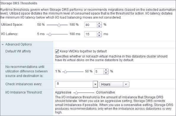
Initial Placement and Regular Balancing
Storage DRS is invoked during the initial placement of disks and on a regular basis at frequent intervals. Whenever a VM is created, cloned, cold-migrated, or Storage vMotioned, Storage DRS attempts to best-place the disks to balance the space and the I/O across the datastore cluster. This mean VMs are balanced across datastores from the outset, and it can simplify and expedite the provisioning process because you know vCenter has already calculated the best-fit for the VM without the need for manual calculations. Instead of specifying a datastore, you select the appropriate datastore cluster, and Storage DRS intelligently decides the best home for the VM. Even if I/O balancing has been disabled for regular balancing, the I/O levels are still considered during the initial placement to ensure that a new VM isn't placed on a heavily loaded datastore.
The frequent and ongoing balancing of the datastores after the initial placements ensures that as disks grow and new I/O loads are added, any imbalances that result are dealt with. The I/O latency is evaluated every eight hours with recommendations made every day, and the space usage is checked every two hours. Even if there isn't enough space or I/O capacity in a destination datastore, Storage DRS can move smaller VMs around to create suitable space. Ongoing balancing also helps when additional datastores are added to the datastore cluster, so that the additional capacity and potential I/O use are absorbed by the cluster and VMs can quickly start to take advantage of it.
Storage DRS's initial placement is arguably the most immediate and beneficial feature, even if doesn't sound as compelling as automated load-balancing. It makes the work of configuring datastore clusters instantly apparent, without the onerous testing that most organizations will run before being comfortable with automated load-balancing. Initial placement helps prevent most storage bottlenecks from the outset. It provides a more scalable, manageable design.
Automation level
There are two automation levels for Storage DRS in a datastore cluster:
- No Automation (Manual Mode)
- Fully Automated
Unlike host DRS clusters, there is no halfway Partially Automated setting, because a datastore cluster's automation level doesn't affect the initial placement. The initial placement is always a manual decision, although it's simplified with the aggregated datastore cluster object and best-fit recommendation.
Fully Automated means all ongoing recommendations are automatically actioned. Manual Mode is safe to use in all cases, and this is where most organizations should start. It allows you to see what would happen if you enabled Fully Automated mode, without any of the changes actually occurring. It's advisable to run under Manual Mode until you understand the impacts and are happy with the recommendations Storage DRS is making. After checking and applying the recommendations, you can turn on Fully Automated mode if it's deemed suitable.
If there are concerns regarding a Fully Automated mode implementation impacting the performance of the hosts or storage arrays during business hours, it's possible to create scheduled tasks to change the automation level and aggressiveness. This allows you to enable the Fully Automated mode out-of-hours and on weekends, to increase the likelihood that migrations happen during those times and to reduce the risk of clashing with performance-sensitive user workloads.
Individual VMs can also be set to override the cluster-wide automation mode. This gives two possibilities: set the cluster to Manual Mode and automate a selection of VMs (and potentially disable some); or, alternatively, set the cluster to Fully Automated but exclude some VMs by setting them to Manual or Disabled. When you disable a VM, its capacity and I/O load are still considered by the cluster when making calculations, but the VM is never a candidate to be moved. This allows a granular enough design for applications that should only be moved under guidance or never at all.
Manual Mode lets an organization become comfortable with the sort of moves that Storage DRS might make should it be set to the Fully Automated setting, and it also lets you test the different threshold levels. Before you move from Manual to Fully Automated, take the time to adjust the threshold levels and monitor how the recommendations change. You should be able to draw the levels down so Storage DRS makes useful recommendations without being so aggressive as to affect performance with overly frequent moves.
Maintenance Mode
Storage DRS has a Maintenance Mode, again mirroring the host DRS functionality. Maintenance Mode evacuates all VMs from a datastore by Storage vMotioning them to other datastores in the cluster while following Storage DRS recommendations. Storage DRS ensures that the additional load is suitably spread across the remaining datastores. Just as Storage DRS assisted with load-balancing capacity and performance when a new datastore was being added, Maintenance Mode helps with load-balancing when a datastore is being removed.
Maintenance Mode is useful when entire LUNs need to be removed for storage array maintenance, and it's of particular assistance during a planned rebuild of VMFS datastores to version 5. You can create an initial datastore cluster of VMFS-3 volumes; then, datastore by datastore, you can clear them of VMs with Maintenance Mode, reformat them fresh with VMFS-5, and join them to a VMFS-5–only datastore cluster. As space on the new cluster is created, VMs can be migrated across. This is also an excellent time to upgrade the VMs to the latest VMware tools and VM hardware, replace network and SCSI hardware with VMXNET3 and PVSCSI, and perform any appropriate additional vSphere 5 upgrades to the VMs. This cut-over provides a clear delineation of upgraded VMs residing on the new datastore cluster.
Affinity Rules
Affinity rules in datastore clusters are similar to the rules that can be created in host clusters, except they're used to keep together or separate a VM's disks. Datastore cluster affinity rules allow control of a VM's disks or individual disks. Affinity rules are enforced by Storage DRS during initial placement and subsequent migrations, but they can be broken if a user initiates a Storage vMotion.
By default, an inherent storage affinity rule is in place for all VMs registered in a cluster, which means a VM's disks and associated files will stay together in the same datastore unless you manually split them or create an anti-affinity rule. This makes troubleshooting easier and is in keeping with what vSphere administrators expect to happen. However, three sets of affinity rules are available in datastore clusters, should your design require them:
Although the cluster default is to keep all of a VM's disks together, this restricts Storage DRS's options when it tries to balance the disks as much as possible. If you want the best possible balance of performance and capacity, you can remove the cluster's inherent VMDK affinity or enable it on a per-VM basis. Just be aware that you may increase your risk by spreading a VM across multiple datastores, with a single failure of a datastore likely to affect far more VMs.
If you set the host cluster option to keep all of a VM's swap files on a host's local disk or a specified datastore, then Storage DRS is automatically disabled on those disks.
Storage DRS Impacts
There are certainly circumstances in which you should be wary of enabling all the Storage DRS features. However, as a general rule, you should attempt to aggregate your storage into datastore clusters and set Storage DRS to Manual Mode. This can safely be enabled for workloads, and you immediately take advantage of reduced points of management through the grouping of datastores, the initial placement recommendations, the ability to create affinity rules, and the ongoing recommendations for capacity management.
Although Storage DRS is aware of thinly provisioned disks created by vSphere, it can't recognize array-based thin-provisioned LUNs by default. This doesn't create a problem for vSphere, but could cause over-provisioning issues for the array if it migrated VMs onto disks that weren't appropriately backed by enough storage. One of the VAAI primitives, if it's available with your array, can warn you about the issue and create a vCenter alarm when the array's LUN is 75 percent full.
When a datastore's underlying disk is deduplicated or compressed on the array, Storage DRS is unaware and won't factor this into the migration calculations. When a VM is moved via Storage DRS, it's effectively inflated on the array, even though the space balancing will appear to have been successful to vCenter. The amount of space recovered by a move may not be as much as expected, but Storage DRS will continue to recommend further moves until the required balance is found. This shouldn't cause any issues, but the space won't be truly balanced on the back end until the dedupe or compression job is run again. To lessen the effect, you can plan to apply the Storage DRS recommendations shortly before the array's space-recovery job is next due to commence.
You should be aware of the array's scheduled tasks if you run regular snapshot jobs. After VMs have been moved between LUNs, you should rerun any snapshot jobs to make sure the new layout is incorporated. If you use VMware-aware backup software, check with the vendor to be sure it's Storage vMotion and Storage DRS aware.
In a couple of cases, you should consider turning off some of Storage DRS's features. With the release of vSphere 5.0 and SRM 5.0, VMware doesn't support the combination of SRM-protected VMs being automatically migrated around with Storage DRS. It can leave some VMs unprotected before SRM realizes the disk files have moved. Additionally, Storage vMotion, and by extension Storage DRS, isn't supported by SRM's vSphere Replication (VR) feature.
Use caution when combining Storage DRS's I/O load-balancing with any underlying storage array that uses automatic disk tiering, because the I/O balancing may not work as you expect. Storage DRS finds it hard to categorize the underlying disks' performance because it may be hitting one or more tiers of very different disks. Also, some tiering software works as a scheduled task on the array, which is unlikely to be aligned perfectly with Storage DRS's runs. This again will tend to cause spurious results, which could create non-optimal I/O recommendations.
As a general rule, you should enable Storage DRS for out-of-space avoidance and initial placement whenever possible. However, you should seek advice from your storage vendor with regard to any capacity-reduction or performance-enhancing features and their compatibility with Storage DRS.
Storage Management
In addition to all the performance and capacity enhancements, vSphere's ability to manage storage has grown enormously. These storage-management features have become possible largely due to the adoption by many of the storage vendors of the new storage APIs discussed earlier. The information and efficiencies provided by VAAI and VASA allow for greatly enriched storage-management capabilities.
Datastore Clusters
We've already explained the functionality associated with datastore clusters under the guise of the improved capacity and performance possible with Storage DRS. However, it's worth remembering that datastore clusters also provide a substantial improvement in storage management in vSphere. The ability to reference one cluster object backed by multiple datastores is a significant step in scalable management.
vSphere administrators have grown accustomed to dealing with host resources as a cluster of compute power instead of lots of individual servers. Now datastore clusters provide a similar analogy to vSphere storage.
Profile-Driven Storage
Profile-driven storage, or Storage Profiles as it's commonly called, is a feature that defines tiers of storage grouped by their underlying capabilities. This grouping of storage lets you apply policies and run ongoing compliance checks throughout the VM's lifecycle, allowing for greater levels of automation, scalability, and discoverability. During VM provisioning, datastores or datastore clusters can be chosen more appropriately when you have a better understanding of the capabilities of each.
Datastore Capabilities
The profile-driven storage tiers can be designated in one of two ways:
If VASA information is available to vSphere, then the process of tagging datastores is automatically provided for you. However, at the time of writing, there is little out-of-the-box support for this, and each vendor implements the capabilities in its own way. If all your storage is provided by one vendor and one model series, then the VASA information can be an invaluable timesaver. VASA not only provides the information but also associates it with the appropriate datastores. You still have to create the Storage Profiles to assign the tagged datastores to the VMs.
If you're dealing with a very mixed environment, or a VASA plugin is unavailable or doesn't provide the required detail, then you can define your own classifications to suit your individual needs. You'll need to create the profiles and then manually associate them with each applicable datastore. The ability to define your own storage tiers means you can use VASA-capable arrays to support this feature, and any array on VMware's HCL can be defined manually.
VASA information describes capabilities such as RAID types, replication, thin provisioning, compression, and deduplication. User-defined capabilities provide the capacity to include datastore tagging based on non-array-specific datastore implementations in an organization, such as backup levels or DR protection and replication levels.
It's common to label such tiers with monikers like Gold, Silver, and Bronze. You should be cautious with naming your datastore-capable tiers generically, because they often have subtly different connotations between teams and between functional use cases. If you can drive a disciplined strategy across the business, where the same VMs will be Silver for DR replication, VM performance, backup RPO/RTO, disk capacity, array LUNs, network QoS, and support SLAs, then basing your vSphere storage tiers on this structure makes obvious sense. However, if you're commonly faced with application exceptions here, there, and everywhere, we recommend that each objective have different naming conventions. The meaning of Gold, Silver, or Bronze is often different for everyone.
VM Storage Profiles
The VM Storage Profiles depend on how you intend to group your VMs and what you intend to use profile-driven storage for. There are countless ways to classify your VMs. Again, and definitely confusingly, a common approach is to group and label them as Gold, Silver, and Bronze. For the same reasons expressed in the previous section, this is rarely a useful naming strategy. Defining the Storage Profiles with clear descriptions is more practical and user-friendly. How you group the VMs is a more interesting design choice.
Some typical VM Storage Profile groupings you can create are based on the following:
- Application
- Business criticality
- Department
- Performance demands
- VMDK-specific categorizations
Once the VM Storage Profiles are created, they can be mapped to datastore capabilities. You can map Storage Profiles one-to-one with a datastore capability, with one-to-many meaning a single capability that can stretch multiple profile use cases (for example, all RAID 1/0 datastores can be used by four different application groups); or, less likely, you can use a many-to-one case (for example, both RAID 5 or RAID 6 storage can be used for a particular department's VMs).
When the VM Storage Profiles have been created and the datastores have been classified, the profiles are automatically attached during a new VM's deployment. The profiles are only a guide; the destination is still a user's choice, and as such incompatible datastores or datastore clusters can be selected. VM Storage Profiles aren't automatically and retrospectively fitted to existing VMs. Those VMs that already exist must be classified manually, to ensure that they're on the correct type of storage and their future compliance can be checked.
Compliance
Storage Profiles are useful in easing the provisioning of new VM, and they allow compliance checking at any stage in the future. The compliance reports identify any VMs and any VMDK disks that aren't stored on an appropriate datastore.
Storage Profile Benefits
Storage Profiles bring a profile-based system to the storage decisions at the time of VM creation. This minimizes the per-VM planning required and increases the likelihood that the VM will be placed on the right type of storage from the outset. Whereas datastore clusters ensure that in a collection of similar datastores, the best datastore is chosen for I/O and capacity reasons, Storage Profiles help you pick the right type of datastore across differently backed options. As a simple example, when you deploy a VM, the Storage Profile helps you choose between the datastores (or datastore clusters) that are replicated and those that aren't; but datastore clusters let you choose the best replicated datastore.
Profile-driven storage can assist when datastore clusters are created. Datastore clusters work most efficiently as vCenter objects when they group similar datastores together. Profile-driven storage tiers help to identify those datastores that are backed by the most similar LUNs. When a VM is matched to a Storage Profile, a datastore cluster can be presented instead of individual datastores.
Storing different VMDK disk types on differently backed datastores is made much less complex with Storage Profiles. It's possible to split each VM's disk into categories; you can do this by applying profiles down to the VMDK level. It allows for subsequent checking and remediation to ensure ongoing compliance. It's now feasible to split guest OS disks onto different datastores in a way that is manageable at scale. Be aware that Storage DRS balancing is disabled for VMs split across multiple datastore clusters. As an example, consider these datastore clusters:
Clearly, applying this level of definition would be time-consuming; but if your storage needs to be managed in such a granular fashion, then profile-driven storage is an invaluable toolset.
Datastore and Host Cluster Designs
Prior to the emergence of datastore clusters in vSphere 5, the single aspect of host cluster sizing was relatively straightforward. Chapter 8 looks at the classic discussion of cluster sizing, i.e. one large cluster of many hosts, or several smaller clusters with fewer hosts in each. There are advantages and disadvantages of each approach, and different circumstances (the functional requirements and constraints) call for different designs. Before vSphere 5, each host cluster would normally be connected to multiple datastores, and the recommended practice of ensuring every host in the cluster was connected to every datastore meant DRS was as efficient as it could be.
As we've just seen, datastore clusters have a similar premise. You can have one datastore cluster of many datastores, or several datastores clusters each containing fewer datastores. Taken in isolation, host clusters and datastore clusters each present a complex set of design decisions. But the two-dimensional aspect of matching datastore clusters to host clusters can make the design exponentially more convoluted. For example, it is entirely feasible to have one host cluster connected to multiple datastore clusters. Alternatively, many host clusters could be attached to only one datastore cluster.
Add in the complexity of multiple arrays: potentially one datastore cluster backed by multiple storage arrays, or conversely a single array supporting multiple datastore clusters. Also, consider the conundrum that datastore clusters aggregate datastores, so looking another layer down, for each datastore cluster do you have a few large datastores or many more datastores that are smaller in size? Where do vDS boundaries align to each of these? Clearly, there are so many factors to consider such as the size of the VMs (storage capacity, storage performance, vCPU, vRAM, vNIC connectivity), the storage arrays (performance, capacity, protocols, functionality such as VAAI primitives, connectivity), and hosts (CPUs, cores, RAM, storage and network connectivity) that each design will need very careful analysis; there is never one design that will fit all situations.
So how do we align datastore and host clusters? There are two crucial aspects to consider which help clarify these choices. There are multiple layers spanning out from the VMs. Each VM needs host resources (vCPUs and vRAM) and storage resources (VMDKs). From the VM, they must run on a host which in turn runs in a host cluster which is contained in a datastore object. That VM's VMDK disks are stored in a datastore, which can be part of a datastore cluster which is contained within the same datastore object. So to understand the datastore and host cluster requirements it is critical to look carefully at the VMs in the context of the datacenter object. Those are the two foundational elements that will have the strongest influence. A holistic overview of all the VMs in a datacenter will drive the architecture of the interim layers. From this point the datastore clusters and host clusters can be designed on their own merit. But remember that the most efficient solution is likely to be one that aligns both cluster types, whether that is one host cluster and one datastore cluster in the datacenter, or aligned multiple clusters thereof, if cluster scaling become an issue.
There are hard limits on these logical constructs that will shape and potentially restrict the optimal configuration. For example, in vSphere 5.1 there is a maximum of 32 datastores in each datastore cluster, a maximum of 32 hosts per host cluster, and no more than 64 hosts to each datastore. There are also numerous limits to the VMs and their components against host and storage resources.
If there are overriding reasons to segregate VMs into one or both cluster types, then maximal cross-connectivity will lessen any design restrictions. For example, if you decide you need two host clusters (one full of scaled up hosts, the other scaled out), and three datastore clusters (one from your legacy SAN, one from fast SSD datastores, and one from the SATA pool), then try to have all hosts from both host clusters connected to all datastores in all datastore clusters. This provides the most technically efficient scenario for DRS, Storage DRS, HA, DPM, etc; considering the cluster divisions you mandated.
vSphere Replication
VMware's Site Recovery Manager (SRM) version 5.0 that was released in 2011 introduced in-built replication to asynchronously copy VMs to a recovery site. This removed the dependence on storage array replication that had been a prerequisite and allowed the hosts to handle the disk copying.
vSphere 5.1 includes this replication as a native feature without the need for SRM. This allows the hosts to provide basic failover protection for VMs without any inherent features in the storage arrays. This provides a basic but cost effective method to copy VMs offsite for DR purposes without involving complex matching of arrays across sites (or intra-site). vSphere replication is included with Essentials Plus and above licenses, and so provides a limited solution that even SMB customers can utilize. vSphere replication doesn't include SRM capabilities like automation, orchestration, multi-VM recovery, reporting, and so on.
The vSphere replication is configured on a per VM basis, and includes Windows guest OS and application quiescing via the VM's VMware tools support for Microsoft VSS. The replication can take place between any type of vSphere supported storage; VMFS, NFS, local storage, except Physical RDMs. Unlike most array based storage replication, there are no requirements to change the storage layout or configuration. Enabling this on each VM is non-disruptive and only delta disk changes are transferred. Because it uses a special vSCSI filter agent it doesn't prevent replicating VMs with snapshots or interfere with VADP CBT backup-type applications. Any snapshotted disks are committed on the destination so no rollback is possible. Only powered-on VMs get replicated and FT and linked clone VMs can't be protected. VMs must be at least hardware version 7.
Although this feature was made available with vCenter 5.1, the replication agent required has been included since ESXi 5.0, so any vSphere 5 hosts are ready. The minimum RPO time possible for each VM is 15 minutes depending on the bandwidth available and the rate of data change. Although multiple sites can be protected, each vCenter can only have one vSphere replication appliance which limits you to one recovery site per vCenter instance. A maximum of 500 VMs can be protected in this way. vSphere replication is compatible with vMotion, HA, DRS, and DPM, but not with Storage vMotion or Storage DRS.
Summary
Now that you understand the elements that make up the storage landscape, your design should consider all four primary factors (availability, performance, capacity, and cost) and reflect the importance of each.
Availability is likely to be very important to the solution unless you're designing storage for a noncritical element such as a test lab. Even what may be considered secondary nodes, such as DR sites, need appropriate redundancy for high availability.
Performance is probably the key to any good storage design these days (high availability is almost taken as a given and doesn't need as much consideration—just do it). With advances in storage devices, it's easy to pack a lot of data onto a relatively small number of disks. You must decide how many IOPS your VMs need (and will need going forward) and use that number to design the solution. You can rely on spindles or consider some of the vendor's new technologies to ensure that performance will meet your requirements. Centralized company datacenters, headquarter buildings, and anywhere with large VDI implementations or intensive database servers will doubtlessly be avid consumers of these performance enhancements.
Capacity must always be considered, so the ability to assimilate your data requirements and understand future growth is very important. An appreciation of this will guide you; but unlike with performance, which can be difficult to upgrade, your design should include strategies to evolve capacity with the business's needs. Disks grow in size and drop in price constantly, so there is scope to take advantage of the improvements over time and not overestimate growth. Capacity can be very important—for example, smaller offices and remote branch offices may consider capacity a crucial element, even more important than performance, if they're only driving large file servers.
Cost will always dictate what you can do. Your budget may not be just for storage, in which case you have to balance it against the need for compute power, licensing, networking infrastructure, and so on. Most likely the funds are nonnegotiable, and you must equate the factors and decide what the best choices are. You may have no budget at all and be looking to optimize an existing solution or to design something from hand-me-downs. Remember in-place upgrades and buy-back deals. There is always a chance to do more for less.
In addition to the fundamentals, other design aspects are worth considering. For example, before you purchase your next SAN, you may ask yourself these questions:
- How easy is this solution to roll out to a site? How easy is it to configure remotely? Is any of it scriptable?
- Physically, how large is it? Do you have the space, the HVAC, the power, the UPS, and so on?
- How is it managed? What are the command-line and GUI tools like? Can multiple arrays be managed together, and managed with policies? How granular is the security?
- What are the reporting features like?
- How easy is it to troubleshoot, upgrade firmware/OS, and add extra disk enclosures?
- Is there any vCenter integration? Are there any special plug-ins?
Extra array functionality may be required, but that's out of scope of this chapter. For example, things like SAN replication and LUN snapshots can play a part in other designs such as backups, DR, application tiering, and so on. Every situation is different.
Planning for the future is normally part of an overall design: you must prepare for how storage will grow with the business. Think about how modular the components are (controllers, cache, and so on), what the warranty covers, how long it lasts, and what support levels are available.
Incorporate the new storage functionalities in vSphere 5 to take advantage of hardware offloading as much as possible. Use the enhanced manageability through datastore clusters with their Storage DRS automation, and make smarter administrative choices with profile-driven storage policies and compliance checking.
Finally, take as much time as possible to pilot gear from different vendors and try all their wares. Use the equipment for a proof of concept, and test each part of your design: protocols, disks, RAID groups, tiering, and so forth. You may be able to clone all or at least some of your production VMs and drop them onto the arrays. What better way to validate your design?