Negative Control

 

Introduction to Exposure

Measuring, controlling and correcting film exposure

Taking focus and adequate depth of field for granted, film exposure and development are the most significant controls of negative quality. In this chapter, we will cover the fundamentals of film exposure and its control. Film development and a closer look at the Zone System, which combines exposure and development, are covered in following chapters.

Photographic exposure is the product of the illumination and the time of exposure. In 1862, Bunsen and Roscoe formulated the reciprocity law, which states that the amount of photochemical reaction is determined simply by the total light energy absorbed and is independent of the two factors individually. This can be expressed as:

H = E · t

where ‘H’ is the exposure required by the emulsion depending on film sensitivity, ‘E’ is the illuminance, or the light falling on the emulsion, controlled by the lens aperture, and ‘t’ is the exposure time controlled by the shutter. The SI unit for illuminance is lux (lx), and exposure is typically measured in lux-seconds (lx·s). This law applies only to the photochemical reaction and the formation of photolytic silver in the emulsion during exposure. It does not apply to the final photographic effect, which is also controlled by the choice of developer and film processing and is measured in density.

Exposure is largely responsible for negative density. Ultimately, our goal is to provide adequate exposure to the shadows, allowing them to develop sufficient density to be rendered with appropriate detail in the print. In all but a few cases, we have full control over altering H, E or t to balance both sides of the equation. If, for example, a given lighting condition does not provide enough exposure, then a more sensitive film could be used, the aperture could be opened to increase the illumination, or the shutter speed could be changed to increase the exposure duration. Illumination and exposure time have a reciprocal relationship, as one is increased and the other decreased by the same factor, the exposure remains constant. Consequently, the law is called the reciprocity law and any deviation from it is referred to as reciprocity failure.

fig.1       Rounded-off values for film speed, aperture and exposure times are incremented in stops, so when one is increased and another is decreased by the same factor, the total exposure remains constant.

Fig.1 shows a table of standard values for film speed, lens aperture and exposure time. The table uses increments of 1 stop, which reflects a change in exposure by a factor of two. A change of one variable can be easily compensated for by an adjustment in one of the other variables. If, for example, the aperture is closed from f/16 to f/22, then this halving of exposure can be adjusted for by either changing the shutter speed from 1/4 s to 1/2 s or by choosing a film with a speed of ISO 400/27° instead of ISO 200/24°.

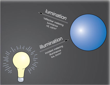
fig.2       Illumination is the light falling onto a surface. It is measured as illuminance ‘E’ (lux or lm/m2) by an ‘incident’ lightmeter. Lumination is the light emitted or reflected from a surface, and it is measured as luminance ‘L’ (nits or cd/m2) by a ‘reflected’ lightmeter.

Whenever finer increments are required, it is customary to move to 1/3-stop increments. These values are given in the table for film speeds from ISO 25/15° to 800/30°. Manual shutter speed dials are typically not marked in increments this fine, but most electronic shutters are capable of incremental adjustments. Manual 35mm-lens apertures rarely provide increments finer than 1 stop, but many medium-format cameras provide 1/2-stop increments and large-format lenses provide 1/3-stop increments as a standard. Some lightmeters offer readings as fine as 1/10 stop, but this increase in resolution is mostly useful for equipment and material testing and has little value for practical photography. You will find more detail on this subject in the chapters on equipment and ‘Quality Control’.

fig.3       Exposure values (EV) are shorthand for aperture/time combinations to simplify meter readings. The equations on the left show the mathematical relationship, where ‘N’ is the lens aperture in f/stops, and ‘t’ is the exposure time in seconds.

EVs

In 1955, the term exposure value (EV) was adopted into the ISO standard. The purpose of the EV system is to combine lens aperture and shutter speed into one variable. This can simplify lightmeter readings and exposure settings on cameras. EV0 is defined as an exposure equal to 1 second at f/1. Fig.3 provides a table covering typical settings, and with it, a light-meter EV reading can be translated into a variety of aperture and shutter speed combinations, while maintaining the same exposure. Each successive EV number supplies half the exposure of the previous one, following the standard increments for film speed, aperture and exposure time. This makes EV numbers an ideal candidate to communicate exposures in the Zone System, since zones are also 1 stop of exposure apart from each other.

Most lightmeters have an EV scale in one form or another. Usually, a subject reading is taken and an EV number is assigned to that reading. This EV number can be used for exposure records and an appropriate aperture/time combination can be chosen depending on the individual image requirements. Some camera brands allow for this EV number to be transferred directly to the lens. Aperture ring and shutter-speed settings can then be interlocked with a cross coupling button, and different combinations can be selected, while maintaining a given EV number and constant film exposure. All Hasselblad CF-series lenses feature this convenient EV ‘interlock button’.

EVs are shorthand for aperture/time combinations and, therefore, independent of film speed. However, a change in film speed may require a different aperture/time combination and, therefore, a change in EV. As an example, let’s assume that a spotmeter returned a reading of EV10 for a neutral gray card, and a moderate aperture of f/8 is chosen to optimize image quality. From fig.3, we see that a shutter speed of 1/15 s would satisfy these conditions. Let’s further assume that we would be much more comfortable with a faster shutter speed of 1/60 s, but we don’t want to change the aperture. The solution is a change in film speed from ISO 100/21° to 400/27°, where the faster film allows f/8 at 1/60 second. Again from fig.3, we see that this combination is equal to EV12. Changing the film speed setting on the meter from ISO 100/21° to 400/27° will result in a change of measured EV to maintain constant exposure.

Some meters make fixed film speed assumptions while measuring EVs. The Pentax Digital Spotmeter, for example, assumes ISO 100/21 at all times. This meter will not alter the EV reading after a film speed change, and due to its particular design, this does not cause a problem. However, it is important to note that some meters simply return a light value (LV) instead of an exposure value (EV). We can still use their exposure recommendations in form of aperture and shutter speed, but LVs are only numbers on an arbitrary scale, measuring subject brightness, and must not be confused with EVs.

Reciprocity Failure

Reciprocity law failure was first reported by the astronomer Scheiner in 1889. He found an inefficiency in the photographic effect at relatively long exposure times, common in astronomical photography. Captain W. Abney reported a similar effect in 1894 at extremely brief exposure times, and the astronomer Karl Schwarzschild (1873-1916) was the first to conduct a detailed study on film sensitivity at long exposure times in 1899. To his credit, the deviation from the reciprocity law, due to extreme exposure times, is often referred to as the ‘Schwarzschild Effect’.

fig.4       The reciprocity law only applies to a limited range of exposure times. Outside of this range, the reciprocity law fails significantly, and an exposure correction is necessary to produce a given negative density.

(graph based on Kodak TMax-400 reciprocity data)

Strictly speaking, the reciprocity law does not hold at all. Every aperture/time combination, theoretically providing the same exposure, creates a different photochemical reaction, and subsequently, a different negative density. Reciprocity failure can be represented graphically as shown in fig.4. If the reciprocity law held, this graph would give a straight horizontal line, but the actual curve is characterized by a minimum, which corresponds to an optimum illumination and most efficient exposure. At the minimum, the smallest amount of illumination is required to produce a given density. The curve rises at illuminance values above and below the optimum, which indicates that an exposure correction is necessary to achieve the required negative density.

The reciprocity law only applies, within reason, to a limited range of exposure times. Outside of this range, the reciprocity law fails significantly for different reasons. At very brief exposure times, the time is too short to initiate a stable latent image, and at very long exposure times, the fragile latent image partially oxidizes before it reaches a stable state. However, in both cases, total exposure must be increased to avoid underexposure. Schwarzschild amended the equation to calculate exposure to:

H = E·t^p

where ‘H’ is the exposure, ‘E’ is the illuminance, ‘t’ is the exposure time, and ‘p’ is a constant. It was later found that ‘p’ deviates greatly from one emulsion to the next and is constant only for narrow ranges of illumination. Consequently, it is more practical to determine the required reciprocity compensation for a specific emulsion through a series of tests.

In my type of photography, brief exposure times are rare, but reciprocity failure due to long exposure times are more the rule than the exception. Modern films, when exposed longer than 1/1,000 second or shorter than 1/2 second, satisfy the reciprocity law. Outside of this range, exposure compensation is required to avoid underexposure and loss of shadow detail. Due to their unique design, Kodak’s TMax films suffer far less from reciprocity failure than standard emulsions like Delta, FP4 or Tri-X, but they also require exposure increases to maintain optimum negative quality.

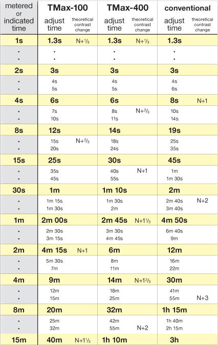
fig.5       This reciprocity compensation table provides exposure and development suggestions for several film types. The contrast changes are based on theoretical values and must be verified by individual tests. Make yourself a copy and keep it in the camera bag as a reference.

Fig.5 shows recommended exposure increases for a few film types. The table is a compilation of suggestions made by John Sexton and Howard Bond, combined with my own test results. The recommendations for conventional film were tested with Ilford’s FP4, and I would not hesitate to use them for other conventional grain films. I have used all values up to 4 minutes of metered time and never experienced any significant exposure deviations. They are offered as a starting point for your own tests, but they are likely to work well as is. Find the lightmeter indicated exposure time in the left column and increase the exposure time to the ‘adjusted time’ of the film type in question. Adjusted times above one hour must be reviewed with caution. Few lighting conditions are constant over such a long period of time.

Fig.5 is based on the preferred method of compensating for reciprocity failure with increased exposure time. Of course, using an increased lens aperture could be an option too. It might even be easier, when final exposure times are between 1 and 2 seconds, which are hard to time accurately. However, in general, it doesn’t solve the problem, it just changes it. Let’s say you are using a conventional film, and you need f/22 for the desired depth of field. The lightmeter suggests an exposure time of 30 seconds, and you see from fig.5 that this time has to be increased to 2 minutes in order to compensate for reciprocity failure. This is equivalent to a 2-stop increase, and you might be tempted to just increase the aperture to f/11. This will have two negative effects. First, you will have reduced the depth of field significantly, and that in itself may not be acceptable. Second, the lightmeter will now suggest an exposure time of 8 seconds, and according to fig.5, the reciprocity troubles are far from over. The new exposure still requires an increase in exposure time to 10 seconds, and we have not gained much.

How can this be? Didn’t we just compensate for that? No, we didn’t. Let’s not forget that we are dealing with very long exposure times here. The reciprocity law is no longer applicable. A 2-stop increase in time is not equal to a 2-stop increase in illumination beyond 1 second of exposure time. By increasing illumination, we shortened the exposure time and reduced reciprocity failure, but we did not eliminate it. Using aperture changes instead of exposure time alterations to compensate for reciprocity failure is possible, but it is usually not very practical and would require a different table.

fig.6       In this example, the reciprocity failure compensation has ‘saved’ the shadow densities, but increased highlight densities to the point that development contraction is required. Development compensations are explained in ‘Development and Film Processing’.

fig.7       In this example, the compensation for reciprocity failure had the welcome side effect of elevating the midtones, and a development expansion to achieve a similar effect is not required.

One unwelcome side effect of reciprocity failure and its compensation is a potential increase in negative contrast. This increase in contrast is due to the under-exposure of the shadows during reciprocity failure, or an unavoidable overexposure of the highlights when it is compensated for with additional exposure. In other words, when subject illumination is very low, exposure times are long, reciprocity failure is experienced, and shadow densities will suffer first. Fig.5 is designed to take this into account by increasing the exposure time so the appropriate shadow density can be maintained, but the highlight zones will receive this increased exposure too, although they may not need it at all.

As you will see in coming chapters, all of my exposure efforts aim for a constant film density in Zone I·5, and all of my film development is customized for Zone VIII·5. According to the Zone System, Zone VIII·5 receives 128 times the exposure of Zone I·5 under normal circumstances. This may be enough illumination for the highlights to experience no reciprocity failure at all, or at least, at a reduced rate. Therefore, the increased exposure time needed for the shadows will cause an overexposure of the highlights, and increased contrast is the result. If the highlights themselves are not affected by reciprocity failure, then every doubling of exposure time will elevate the highlights by one zone and increase the overall contrast by an equivalent of N+1.

All other tonalities are affected to a lesser extent. As a rule of thumb, Zones I to III will need the entire exposure increase to compensate for reciprocity failure and do not experience a contrast increase. Zones IV to VI will use half of the exposure towards compensation and the rest will elevate each zone by half a stop per exposure doubling. Finally, Zones VII to IX will receive one full zone shift for every exposure time doubling involved, because reciprocity correction is not needed for the highlights. These tonal shifts must be considered when overall zone placement is visualized during regular Zone System work.

Let’s use the previous example again, where reciprocity failure of a conventional film required an exposure time increase from 30 seconds to 2 minutes. In this case, the shadows needed the additional 2 stops of exposure to maintain adequate negative density, but as seen in fig.6, the highlights did not need the exposure and will develop unnaturally dense. This is reflected in the ‘contrast change’ column by the term ‘N+2’. The only remedy available to compensate for this increase in contrast is a decrease in development time in order to keep highlight densities down. Fig.5 provides information on how much contrast compensation is required, but the details of contrast control through development and its practical application will be discussed in the next chapter.

The next example, fig.7, will illustrate another situation. Let’s say we are inside a dark church on a dull day and the lighting is so poor that the meter indicates a 15-minute exposure at the selected aperture. The camera is loaded with FP4, and fig.5 suggests an exposure time increase to 3 hours. From the contrast column, we get the information that image highlights will receive about 3.5 doublings of exposure, but in this example, the scene does not have any highlights. The lightest part of the image is a light gray wall falling onto Zone VI, and therefore, only about half of the contrast increase will have an effect elevating the wall to a low Zone VIII. This situation may fit our visualization of the scene well and we decide that no contrast compensation is required.

Eastman Kodak claims that their TMax films do not require any contrast compensation due to reciprocity failure. Ilford’s tests with FP4 revealed a slight contrast increase, but far less than the theoretical values in fig.5. This can be explained with the fact that many film emulsions have fast (toe) and slow (shoulder) components, which are responsible for different parts of the characteristic curve. These components fail the reciprocity law to different degrees and the theoretical values in fig.5 are, therefore, most likely overstated. They should be verified through individual film/developer tests.

Contrast Control

Negative contrast is typically controlled with film development. However, for very long exposure times, there is a simple technique to reduce the subject brightness range and avoid excessive negative contrast by selectively manipulating the exposure itself.

When composing a low light level or nighttime scene, the light source itself can become part of the image. A street light, a light bulb or even the moon are part of the scene and are so bright, compared to the rest of the image zones, that they end up ruining the image with severe flare or are burned out beyond recognition. For this reason, I carry a simple black card as seen in fig.8 in my camera bag. It can be made from thick cardboard or thin plastic sheeting, but it should be made from matt black material. Use it to dodge the light source during a portion of the film exposure time. I practice the process, while either looking through the viewfinder or onto the ground glass, until I feel confident enough to cover the area in question with the card at arm’s length. During the actual exposure, the card is constantly in motion to avoid any telltale signs, much like when dodging a print in the darkroom. Covering the light source for half the exposure time will lower it by one zone. This is not an accurate procedure, and it is one instance where I bracket my exposures.

fig.8       A card can be used to dodge bright highlights during very long exposures.

Spectral Sensitivity

Electromagnetic radiation, ranging in wavelength from about 400-700 nm, to which the human eye is sensitive, is called light. One often overlooked source of unexpected results in monochrome photography is the fact that our eyes, lightmeters and films have unmatched sensitivities to these different wavelengths of the visible spectrum. Fig.9 combines a set of idealized curves showing the typical spectral sensitivities of the human eye, the silicon photo diode, as used in the Pentax Digital Spotmeter, and a typical panchromatic film.

fig.9       Eyes, equipment and materials, all with different spectral sensitivities, are involved in the photographic process. This can make realistic tonal rendering a hit-or-miss operation.

Our eyes have their peak sensitivity at around 550-560 nm, a medium green. This sensitivity diminishes towards ultraviolet and infrared at about the same rate, following a normal distribution and forming a bell curve. Lightmeters depend on light sensitive elements and are, as of this writing, mostly made of either silicon or selenium. Unfortunately, the sensitivities of their diodes and cells do not accurately simulate human vision, because they are more sensitive towards blue and red than the eye.

Film technology has come a long way since its early days. The first emulsions were only sensitive to ultraviolet (UV) and blue light. Improvements led to the introduction of orthochromatic materials, which are also sensitive to green light, but are still blind to red. Portraits as late as the 1930s show people with unnaturally dark lips and skin blemishes as a result. Eventually, the commercialization of panchromatic film in the 1920s offered an emulsion that is sensitive to all colors of light. These films have the ability to give gray tone renderings of subject colors closely approximating their visual brightness, but despite all efforts, panchromatic emulsions still have a high sensitivity to blue radiation. UV radiation, however, is less of a concern, because any glass in the optical path, as in lenses, filters out most of it.

fig.10     A Yellow (8) filter absorbs most of the blue light, enabling panchromatic film to closely match the spectral sensitivity of human vision to daylight.

Have you ever had a print in which the sky appears to be much lighter than you remember it? Fig.9 offers a potential explanation. The eye is far less sensitive towards blue than the film is. What we see as a dark blue sky, the film records as a much lighter shade of gray, minimizing contrast with clouds and often ruining the impact in scenic photography.

Again from fig.9, we see that lightmeters are more sensitive towards red than film is. Using a spotmeter, taking a reading of something predominately red and placing it on a particular zone may render it as much as one zone below anticipation.

I have tested the Pentax Digital Spotmeter and the Minolta Spotmeter F for spectral sensitivity on Ilford FP4. Both gave excellent results for white, gray and yellow material, matched green foliage within 1/3 stop, but rendered red objects as much as 1 stop underexposed. This test result is likely to change using different emulsions, and it becomes clear that matching the spectral sensitivity of lightmeters and films is a rather complex, if not impossible, task. Unless both can be manufactured to match the spectral responses of the human eye, realistic tonal rendering of colored objects will persist to be a bit hit-or-miss.

Filters

Filters provide useful control over individual tonal values at the time of exposure. They are used either to correct to the normal visual appearance or to intentionally alter the tonal relationship of different subject colors, providing localized contrast control. Filters are made from gelatin, plastic or quality optical glass and contain colored dyes to limit light transmission to specific wavelengths of light.

The total photographic effect obtained through filtration depends on the spectral quality of the light source, the color of the subject to be photographed, the spectral absorption characteristics of the filter and the spectral sensitivity of the emulsion. A filter lightens its own color and darkens complementary colors. A red filter appears red because it only transmits red light; most of the blue and green light is absorbed or filtered out. A blue object will record darker in the final print if exposed through a yellow filter, while a yellow object will record slightly lighter through this filter.

Filters are made for various purposes, but we will concentrate on a few color correction and contrast control filters, which are key to monochromatic photography. To specify filters accurately, we will refer to Kodak’s Wratten numbers in addition to the filter color. I consider the use of four filters to be essential, namely Yellow (8), Green (11), Orange (15) and Red (25).

Yellow (8) absorbs all UV radiation and is widely used to correct rendition of sky, clouds and foliage with panchromatic materials. Fig.10 shows how it closely matches the color brightness response of the eye to outdoor scenes, slightly overcorrecting blue sky. Green (11) corrects the color response to match visualization of objects exposed to tungsten illumination and to elevate tonal rendition of foliage in daylight, while darkening the sky slightly. Orange (15) darkens the sky and blue-rich foliage shadows in landscape photography more dramatically than (8) and is also useful for copying yellowed documents. Red (25) has a high-contrast effect in outdoor photography with very dark skies and foliage. It is also used to remove blue in infrared photography.

Since filters absorb part of the radiation, they require exposure increase to correct for the light loss. Fig.11 provides an approximate guide for popular monochromatic filters in daylight and tungsten illumination. You can perform your own tests by using this table as a starting point and a Kodak Gray Card. First, take a picture of the card without a filter. Then, with the filter in place, expose in 1/2 or 1/3-stop increments around the recommended value. A comparison of the negatives will guide you to which is the best exposure correction.

As a last suggestion, take all light readings without a filter in place, and then, apply the exposure correction during exposure. Filters will interfere with the lightmeter’s spectral sensitivity, and incorrect exposures may be the result.

Lens Extension

When a lens is focused at infinity, the distance between lens and film plane is equal to the focal length of the lens. As the lens is moved closer to the subject, it must be moved farther from the film plane to keep the subject in focus. While this increases subject magnification, it also causes the light entering the lens to be spread over a larger area, reducing the illumination. To compensate for the reduction in illumination, the exposure must be increased.

The f/stop markings on the lens are only accurate for infinity focus, but the light loss is negligible within the normal focusing range of the lens. Up to a subject magnification of about 1/10, the effect is smaller than 1/3 stop. However, for lens-to-subject distances of less than 10 times the focal length, exposure correction is advisable.

The subject magnification (m), the exposure correction factor (e) and the required f/stop exposure correction (n) can be calculated as:

where ‘v’ is the lens or bellows extension (the distance between film plane and the rear nodal plane of the lens), ‘u’ is the lens-to-subject distance (the distance between front nodal plane of the lens and the focal plane) and ‘f’ is the focal length of the lens.

fig.11     These are recommended exposure corrections in stops for key B&W filters in daylight and tungsten illumination.

The rear nodal plane is the location from which the focal length of a lens is measured. Depending on lens construction, the rear nodal plane may not be within the lens body. In true telephoto lenses, it can be in front of the lens. In SLR wide-angle lenses, which need to leave enough room for a moving mirror, it is behind the lens. To determine the location of the rear nodal plane with sufficient accuracy for any lens, follow this procedure:

1.   Either set the lens to infinity, or focus the camera carefully on a very distant object. Never point the camera towards the sun!

2.   Estimate the location of the film plane and measure a distance equal to the focal length towards the lens.

3.   The newly found position is the location of the rear nodal plane at infinity focus.

As the lens is moved further away from the film plane to keep the subject in focus, the rear nodal plane moves with it and can be used to accurately measure the lens extension.

The most convenient ways to correct the exposure for lens extension are to use the f/stop exposure correction (n) to open the lens aperture or to extend shutter exposure time. Fig.12 is used to estimate the exposure correction depending on lens extension for common focal lengths without requiring any calculations. Find the intersection of focal length and measured lens extension to determine subject magnification and exposure correction in f/stops. Then, open lens aperture or extend shutter exposure to compensate for the loss of illumination at the film plane.

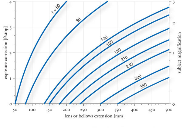
fig.12     Lens or bellows extensions enable subject magnification, but they require an exposure correction depending on focal length of the lens. Many common focal lengths are shown here, and others may be interpolated. Find the intersection of focal length and measured lens extension to determine subject magnification and exposure correction. Then, open lens aperture or extend shutter exposure to compensate for the loss of illumination at the film plane.

In some cases, it may be undesirable to open the lens aperture or impossible to increase the exposure through the shutter mechanism. The exposure correction factor (e) provides an alternative method. Modify the exposure time by multiplying it by the exposure correction factor, compensating for the loss of illumination at the film plane.

Bellows Extension

With view cameras, lens extension is referred to as bellows extension. The terminology change is due to a different camera construction, but the principle of exposure correction and the measurements required are still the same. Nevertheless, the relatively large negative format and the fact that the image on the ground glass and film are the same size enable the use of a simple tool. Fig.13 shows a full scale exposure target and its accompanying ruler. Copy the target (left) and the ruler (right) for your own use. Laminate each with clear tape to make them more durable tools.

The next time you create an image and the subject distance is less than 10 times the focal length, place the target into the scene to be photographed. Measure the diameter of the circle on the ground glass with the ruler, reading off subject magnification and the required f/stop correction. Adjust the exposure by either opening the lens aperture or extending the exposure time accordingly.

fig.13     View camera owners, copy the target and the ruler for your own use. Laminate each piece with clear tape to make a more durable tool. For close-up photography, place the target into the scene, and measure the diameter of the circle on the view screen with the ruler. Determine subject magnification and f/stop correction to adjust exposure by opening lens aperture or extend shutter exposure.

Technically speaking, perfect exposure ensures that the film receives the exact amount of image-forming light to make a perfect negative. Manual exposure control, using handheld lightmeters combined with visualization techniques like the Zone System, is a slow pursuit and not applicable for every area of photography. On the other hand, fully automatic exposure systems yield a high percentage of accurate exposures with average subjects but remove much individualism and creative control. It is the photographer’s decision when to use which system.

 

Development and Film Processing

Controlling negative contrast and other film processing steps

Film development is the final step to secure a high-quality negative. Unlike print processing, we rarely get the opportunity to repeat film exposure and development, if the results are below expectations. In order to prevent disappointment, we need to control film processing tightly. Otherwise, fleeting moments can be lost forever. Once film exposure and development is mastered, formerly pointless manipulation techniques become applicable and, in combination with the Zone System, offer the possibility to manage the most challenging lighting conditions. Many photographers value the negative far higher than a print for the fact that multiple copies, as well as multiple interpretations of the same scene, are possible from just one negative. The basic chemical process is nearly identical to the paper development process, which was covered in some detail in ‘Archival Print Processing’, but a comprehensive understanding is important enough to warrant an additional, brief overview.

Film Processing in General

The light reaching the film during exposure leaves a modified electrical charge in the light sensitive silver halides of the emulsion. This change cannot be perceived by the human eye and is, therefore, referred to as a ‘latent image’, but it prepares the emulsion to respond to chemical development. Chemical development converts the exposed silver halides to metallic silver; however, unexposed silver halides remain unchanged. Highlight areas with elevated exposure levels develop more metallic silver than shadow areas, where exposure was low. Consequently, highlight areas develop to a higher transmission density than shadows, and a negative image can be made visible on the film through the action of the developer. For this negative to be of practical use, the remaining and still light sensitive silver halides must be removed without affecting the metallic silver image. This is the essential function of the fixer, which is available either as sodium or ammonium thiosulfate. The fixer converts unexposed silver halide to soluble silver thiosulfate, ensuring that it is washed from the emulsion. The metallic silver, creating the negative image, remains. Fig.1 shows our recommendation for a complete film processing sequence, which is also a reflection of our current developing technique.

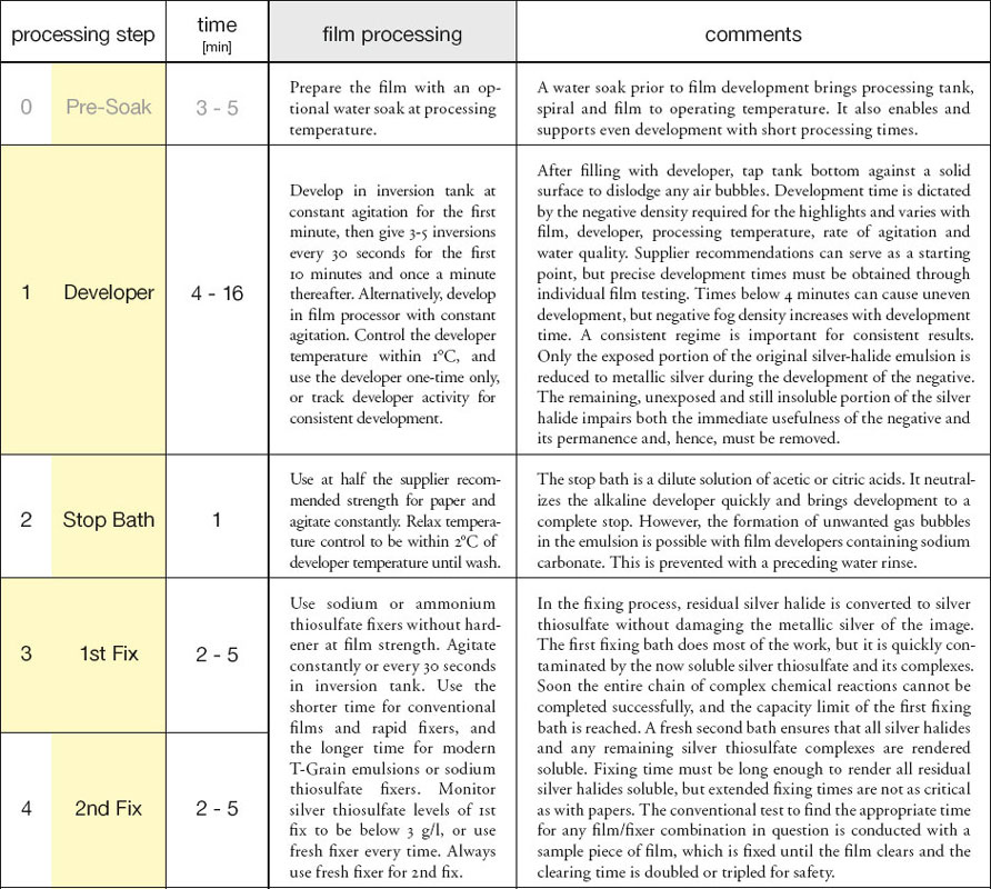
fig.1       Negatives are valuable, because they are unique and irreplaceable. Archival processing, careful handling and proper storage work hand in hand to ensure a maximum negative life expectancy.

Developers and Water

The variety of film developers available is bewildering, and writing about different developers with all their advantages or special applications has filled several books already. The Darkroom Cookbook by Steve Anchell is full of useful formulae, and is my personal favorite. The search for a miracle potion is probably nearly as old as photography itself, and listening to advertising claims or enthusiastic darkroom alche-mists, is not about to end soon. However, I would like to pass along a piece of advice, given to me by C. J. Elfont, a creative photographer and author himself, which has served me well over the years. ‘Pick one film, one developer, one paper and work them over and over again, until you have a true feeling for how they work individually and in combination with each other.’ This may sound a bit pragmatic, but it is good advice, and if it makes you feel too limited, try two each. The point is that an arsenal of too many material alternatives is often just an impatient response to disappointing initial attempts or immature and inconsistent technique. Unless you thrive on endless trial and error techniques, or enjoy experimentation with different materials in general, it is far better to improve craftsmanship and final results with repeated practice and meticulous record keeping for any given combination of proven materials, rather than blaming it possibly on the wrong material characteristics. There are no miracle potions!

Nevertheless, film developer is a most critical element in film processing. A recommendation, based on practical experience, is to begin with one of the prepackaged standard film developers like ID-11, D-76 or Xtol and stick to a supplier proposed dilution. This offers an appropriate compromise between sharpness, grain and film speed for standard pictorial photography. Unless you have reason to doubt your municipal water quality or consistency, you should be able to use it with any developer. However, distilled or deionized water is an alternative, providing additional consistency, especially if you develop film at different locations. Filters are available to clean tap water from physical contaminants for the remaining processing steps, but research by Gerald Levenson of Kodak as far back as 1967 and recently by Martin Reed of Silverprint suggests avoiding water softeners as they reduce washing efficiency in papers.

fig.2       Negative contrast is defined as negative density increase per unit of exposure. The same exposure range can differ in negative density increase according to the local shape of the characteristic curve. The local slope, or gradient, is a direct measure of local negative contrast.

Characteristic Curve, Contrast and Average Gradient

Film characteristic curves were briefly introduced in ‘Introduction to Sensitometry’. They are used to illustrate material and processing influences on tone reproduction throughout the book. They are a convenient way to illustrate the relationship between exposure and negative density, but it is also helpful to have a quantitative method to evaluate and compare characteristic curves. Over the years, many methods have been proposed, mainly for the purpose of defining and measuring film speed. Several have been found to be inadequate or not representative of modern materials and have since been abandoned. The slightly different methods used by Agfa, Ilford, Kodak, and the current ISO standard are all based on the same ‘average gradient’ method.

Negative contrast is defined as negative density increase per unit of exposure. Fig.2 shows how the same exposure range can differ in negative density increase according to the local shape of the characteristic curve. In this example, toe and shoulder of the curve have a relatively low increase in density signified by a gentle slope or gradient, and the gradient is steepest in the midsection of the curve. These local gradients are a direct measure of local negative contrast, but a set of multiple numbers would be required to characterize an entire curve.

The average gradient method on the other hand, identifies just two points on the characteristic curve to represent significant shadow and highlight detail, as seen in fig.3. Here a straight line, connecting these two points, is evaluated on behalf of the entire characteristic curve, while fulfilling its function of averaging all local gradients between shadows and highlights. The slope of this line is the average gradient and a direct indicator of the negative’s overall contrast. It can be calculated from the ratio a/b, which is the ratio of negative density range (a) over log exposure difference (b). The average gradient method is universally accepted, but as we will see in the following chapters, the consequences of selecting the endpoints are rather critical and different intentions have always been a source of heated discussion among manufacturers, standardization committees and practical photographers. At the end of the day, it all depends on the desired outcome and in ‘Creating a Standard’ we define these endpoints to our specifications in compliance with the rest of this book and a practical approach to the Zone System in mind.

fig.3       The average gradient method identifies two points on the characteristic curve representing significant shadow and highlight detail. A straight line connecting the points is evaluated on behalf of the entire characteristic curve.

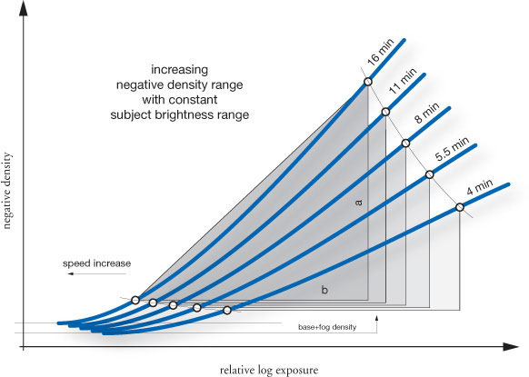
fig.4       Shadow densities change only marginally when development times are altered, but highlight densities change significantly. The average gradient and the negative density range (a) increase with development time, when the subject brightness range (b) is kept constant.

fig.5       The average gradient increases and the subject brightness range (b) decrease with development time, when the negative density range (a) is kept constant.

Time, Temperature and Agitation

Exposure is largely responsible for negative density, but film development controls the difference between shadow and highlight density, and therefore the negative contrast. The main variables are time, temperature and agitation, and controlling development precisely requires that these variables be controlled equally well. Data sheets provide starting points for developing times and film speeds, but complete control can only be achieved through individual film testing, as described in detail through following chapters.

Fig.4 shows how the development time affects the characteristic curve when all other variables are kept constant. With increased development time, all film areas, including the unexposed base, increase in density, but at considerably different rates. The shadow densities increase only marginally, even when development times are quadrupled, where simultaneously, highlight densities increase significantly. This effect is most useful to the Zone System practitioner and can be evaluated from the following two aspects.

First, in fig.4 the subject brightness range (b) is kept constant by fixing the relative log exposure difference between shadow and highlight points. We can see how the negative density range (a) and the average gradient increase with development time. Second, in fig.5 the negative density range (a) is kept constant by fixing the negative density difference between shadow and highlight points. This way, we can see how the average gradient increases, but the subject brightness range (b) decreases with development time.

The last observation is the key to the Zone System’s control of the subject brightness range by accordingly adjusted film development time. The negative density range is kept constant, allowing to print many lighting conditions on a single grade of paper with ease. Other paper grades are not used to compensate for difficult to print negative densities anymore, but are left for creative image interpretation.

One important side effect becomes apparent with both figures. The shadow points, having a constant density above base+fog density, require less exposure with increasing development time, or in other words, film speed increases slightly with development. Consequently, film exposure controls shadow density and development controls highlight density, but we must always remember that film speed varies with development time.

The standard developing temperature for film is 20°C. Photographers living in warmer climates often find it difficult to develop film at this temperature and may choose 24°C as a viable alternative. However, development temperature is a significant process variable, and film development time tests must be repeated for different temperatures and then tightly controlled within 1°C. The temperature compensation table in fig.6 gives reasonable development time substitutes for occasional changes in development temperature. Do not underestimate the cooling effect of ambient darkroom temperatures in the winter or the warming effect of your own hands on the inversion tank. The temperature is less critical for any processing step after development. The above tolerance can be doubled and even tripled for the final wash, but sudden temperature changes must be avoided, otherwise reticulation, a wrinkling of the gelatin emulsion, may occur.

Agitation affects the rate of development, as it distributes the developer to all areas of the film evenly, as soon as it makes contact. While reducing the silver halides to metallic silver, the developer in immediate contact with the emulsion becomes exhausted and must be replaced through agitation. Agitation also supports the removal of bromide, a development byproduct, which otherwise inhibits development locally and causes ‘bromide streaks’.

A consistent agitation technique is required for uniform film development. You can use the recommendations in fig.1 as a starting point, or you can test for proper agitation yourself. Expose an entire negative to a uniform surface placed on Zone VI and develop for the normal time, but using different agitation methods. Increased density along the edges indicates excessive agitation, and uneven or mottled negatives indicate a lack of agitation.

Normal, Contraction and Expansion Development

Normal development creates a negative of normal average gradient and contrast. A negative is considered to have normal contrast if it prints with ease on a grade-2 paper. An enlarger with a diffused light source fulfills the above condition if the negative has an average gradient of around 0.57. A condenser enlarger requires a lower average gradient to produce an identical print on the same grade of paper. We will discuss other practical average gradient targets in detail in the next two chapters, and a table with typical negative densities for all zones is given in ‘Tone Reproduction’.

We saw in fig.5 how the intentional alteration of film development time and average gradient can provide control over the subject brightness range, while maintaining a constant negative density range, which keeps print making from becoming a chore. However, if the alteration is unintentional, then density control becomes a processing error. Film manufacturers have worked hard to make modern films more forgiving to these ‘processing errors’ and have, in turn, taken some of the tonal control away from Zone System practitioners. Nevertheless, even modern emulsions still provide enough tonal control to tolerate subject brightness ranges from 5-10 stops or more.

fig.6       The standard developing temperature for film is 20°C. However, this temperature compensation table gives reasonable development time substitutes for occasional changes in development temperature. For example, developing a film for 10 min at 20°C will lead to roughly the same negative densities as developing it for 7 min at 24°C.

fig.7       In this example, the highlights of a high-contrast scene metered two zones above visualization. N-2 contraction development is used, limiting the highlight densities to print well on grade-2 paper.

fig.8       In this example, the highlights of a low-contrast scene metered two zones below visualization. N+2 expansion development is used, elevating the highlight densities to print well on grade-2 paper.

In a low-contrast lighting condition, the normal gradient produces a flat negative with too small of a density difference between shadows and highlights, and the average gradient must be increased to print well on normal paper. In a high-contrast lighting condition, the normal gradient produces a harsh negative with a negative density range too high for normal paper, and the average gradient must be decreased. The desired average gradient can be achieved by either increasing or decreasing the development time, but appropriate development times must be determined through careful film testing.

In regular Zone System practice, we measure the important shadow values first and then determine appropriate film exposure with that information alone, thereby placing these shadows on the visualized shadow zone. Then, we measure the important highlight values and let them ‘fall’ onto their respective zones. If they fall onto the visualized highlight zone, then development is normal. If they fall two zones higher, contraction development of N-2 must be used to keep the highlight from becoming to dense. On the other hand, if they fall two zones lower, expansion development of N+2 must be used to elevate the highlight densities. Fig.7 and fig.8 show how the tonal values change due to contraction and expansion development respectively, and fig.9 and fig.10 illustrate the concept further.

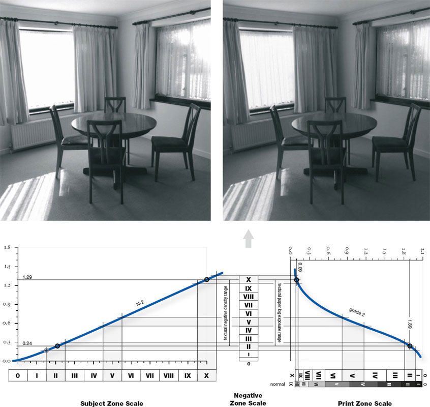
fig.9a    In this high-contrast scene, normal film development was not able to capture the entire subject brightness range, and as a result, some highlight detail is lost with grade-2 paper.

(print exposed for shadow detail to illustrate strong negative highlight density)

fig.9b    N-2 film development extended the textural subject brightness range by two zones. This reduced the overall negative contrast and darkened midtones but avoided a loss of highlight detail.

fig.9c    N-2 film development is used to increase the subject brightness range captured within the normal negative density range.

In fig.9a, shadows at the bottom of the table were measured to determine film exposure. The film was developed for a time, previously tested to cover a normal textural subject brightness range of 6 stops. The print was then exposed to optimize shadow density. However, this high-contrast indoor scene had a subject brightness range of 8 stops, far too much for normal development, and consequently, the negative highlight detail was too dense to register on normal grade-2 paper. fig.9b is from a negative, which received the same exposure, but a contracted N-2 film development reduced highlight densities and allowed for the entire subject brightness range to be recorded on grade-2 paper. This reduced overall negative contrast, darkened midtones and making for a somewhat duller print, but it avoided a loss of highlight detail.

In fig.10a, shadows at the bottom of stairs were measured to determine film exposure. Again, the film was given normal development, and the subsequent print was exposed to optimize shadow density as well. This time, the low-contrast scene had a subject brightness range of only 4 stops, and consequently, the negative highlight detail did not gain sufficient density during normal development to show clear white on normal grade-2 paper. fig.10b is from a negative, which received the same exposure, but an extended N+2 film development increased negative highlight densities, utilizing the entire print density range of grade-2 paper. This increased overall negative contrast, lightened midtones and got rid of muddy and dull highlight detail.

fig.10a  In this low-contrast scene the subject brightness range is small and normal film development will make for a dull print with grade-2 paper.

(print exposed for shadow detail to illustrate weak negative highlight density)

fig.10b  N+2 film development elevated highlight densities by two zones, increasing negative and print contrast. The entire negative density range is used.

fig.10c  N+2 film development is used to decrease the subject brightness range captured within the normal negative density range. Final zone densities depend on the negative and paper characteristic curves, but some trends due to film development are clearly visible in fig.8c and here.

Optional Processing Steps

Film processing is very similar to print processing. Exposed silver halides are developed to metallic silver, unexposed halides are removed from the emulsion, thereby fixing the image and making it permanent, and finally, the film is washed to remove residual chemicals. Fig.1 shows a complete list of film processing steps that lead to negatives of maximum permanence. Depending on individual circumstances, some of these processing steps are optional, but with the exception of washing aid, when applied on a regular basis, they all must be part of the film-development test.

Pre-Soak

A water soak prior to film development keeps sheet film from sticking together when placed into the developer and brings processing tank, spiral and film to operating temperature, but it also causes the gelatin in the film’s emulsion to absorb water and swell. As a consequence, the subsequent developing bath is either absorbed more slowly, extending the development time, or the wet emulsion promotes the diffusion of some chemicals, reducing the development time.

In general, a pre-soak supports a more even development across the film surface and is, therefore, recommended with short processing times of less than 4 minutes. However, when applied, it must be long enough (3-5 minutes) to avoid water stains. The pre-soak partially washes antihalation and sensitizing dyes from the film. This is harmless and helpful in removing a disturbing pink tint from negatives, but when dyes are washed out, useful wetting agents and possible development accelerators are potentially washed from the film as well. This is another reason why the effect of a pre-soak on development time must be tested for each film/developer combination.

Stop Bath

The stop bath is a dilute solution of acetic or citric acid. It neutralizes the alkaline developer quickly and brings development to a complete stop. However, unwanted gas bubbles may form in the emulsion with film developers containing sodium carbonate, which will impede subsequent fixing locally.

This is easily prevented with a water rinse prior to the stop bath, or by replacing the stop bath with a water bath. Please note, however, that development will slowly continue in the rinse or water bath until all active development ingredients are exhausted, or the fixer finally stops development altogether. Some darkroom workers see this as an opportunity to enhance shadow detail slightly, and they propose replacing the stop bath with a water bath as a general rule. Their reasoning is that it takes longer to exhaust the developer in areas of low exposure, and thereby, shadows have a longer developing time in the water bath than highlights.

2nd Fix

In the fixing process, residual silver halide is converted to silver thiosulfate without damaging the metallic silver of the image. The first fixing bath does most of the work, but it is quickly contaminated by the now soluble silver thiosulfate and its complexes. Soon the entire chain of complex chemical reactions can not be completed successfully, and the capacity limit of the first fixing bath is reached. A fresh second bath ensures that all silver halides and any remaining silver thiosulfate complexes are rendered soluble.

Fixing time must be long enough to render all residual silver halides soluble, but extended fixing times are not as critical with film as they are with papers. The conventional test to find the appropriate time for any film/fixer combination is conducted with a sample piece of film, which is fixed until the film clears and the clearing time is doubled or tripled for safety.

Toner

It is recommended to file negatives in archival sleeves and keep them in acid-free containers. This way, they are most likely stored in the dark and the exposure to air-born contaminates is minimized, which means that they are normally better protected than prints. Nevertheless, brief toning in sulfide, selenium or gold toner is essential for archival processing. It converts sensitive negative silver to more stable silver compounds. Process time depends on the type of toner used and the level of protection required. Use only freshly prepared toner, otherwise, toner sediments will adhere to the soft emulsion and cause irreparable scratches on our valuable negatives.

Washing the film prior to toning is a necessity, because excess fixer causes staining and shadow loss with some toners. The wash removes enough fixer to avoid this problem. For selenium toning, a brief 4-minute wash is sufficient, but direct sulfide toning requires a 10-minute wash.

Washing Aid

Applying a washing-aid bath prior to the final wash is standard with fiber-base print processing, and is also recommended for film processing. It makes residual fixer and its by-products more soluble and reduces the final washing time significantly. Washing aids are not to be confused with hypo eliminators, which are not recommended, because they contain oxidizing agents that may attack the image.

Washing aid is one of the few chemicals in film processing that can be used more than once. A brief water rinse prior to its application is recommended; otherwise, residual fixer or toner contaminate the washing aid and reduce its effectiveness. The rinse removes enough fixer and toner to considerably increase washing aid capacity.

Washing the Film

The basic process of film washing is almost identical to washing prints. However, in many ways, film responds to washing more like an RC print, because in both, the emulsion is directly coated to the plastic substrate and not to an intermediate layer of paper fibers, as with fiber-base prints. This makes film washing unique enough to repeat a few key points about washing, in general, and address the specifics of film washing, in particular.

Previously fixed or selenium toned film contains a substantial amount of thiosulfate, which must be removed to give the negative a reasonable longevity or archival stability. The principal purpose of archival washing is to reduce residual thiosulfate to a specified concentration, known to assure a certain life expectancy. This specification has changed over time. In 1993, ISO 10602 called for no more than 0.007 g/m² residual thiosulfate in film across the board. The current standard, ISO 18901:2002, differentiates between a maximum residual thiosulfate level of 0.050 g/m² for a life expectancy of 100 years (LE100) and 0.015 g/m² for a life expectancy of 500 years (LE500). The new standard, therewith, recognizes the different life expectancies of roll and sheet film, most of which are coated on acetate and polyester substrates, respectively. According to the Image Permanence Institute (IPI), an acetate film base has a life expectancy of only 50-100 years, but a polyester base has a predicted life expectancy of over 500 years. Consequently, the LE500 value is only applicable for polyester-base sheet films, since acetate-base roll films don’t last for 500 years.

The old standard assumed that residual thiosulfate levels should be as low as possible. The new standard responds to recent findings, which ironically show that small residual amounts of thiosulfate actually provide some level of image protection. Safe levels of residual thiosulfate vary with the type of emulsion. Fine-grain emulsions have a greater surface-to-volume ratio than large-grain emulsions, and are, therefore, more vulnerable to the same level of residual thiosulfate. This explains why the archival print standard calls for lower residual thiosulfate levels than the LE100 film standard. Print emulsions have a much finer grain than film emulsions.

Film washing is a combination of displacement and diffusion. Initially, the wash water quickly displaces excess fixer by simply washing it off the surface. However, some thiosulfate will have been absorbed by the film emulsion, and it must diffuse into the surrounding wash water, before it can be washed away. As long as there is a difference in thiosulfate concentration between the film emulsion and the wash water, thiosulfate will diffuse from the film into the water. The thiosulfate concentration gradually reduces in the film as it increases in the wash water (fig.11a). Diffusion continues until both are of the same concentration and an equilibrium is reached, at which point, no further diffusion takes place. Replacing the saturated wash water with fresh water restarts the process, and a new equilibrium at a lower thiosulfate level is obtained. The process is continued until the residual thiosulfate level is at, or below, the archival limit.

fig.11a    As long as there is a difference in thiosulfate concentration between the film emulsion and the wash water, thiosulfate will diffuse from the film into the water. This gradually reduces the thiosulfate concentration in the film and increases it in the wash water. Diffusion continues until both are of the same concentration and an equilibrium is reached.

fig.11b    During cascade washing, the saturated wash water is entirely replaced with fresh water each time the equilibrium is reached. This repeats the process of diffusion afresh. Cascade washing is continued until the residual thiosulfate level is at or below the archival processing limit.

For quick and effective film washing, running water is recommended, because water replenishment over the entire paper surface is essential for even and thorough washing. A continuous supply of water also keeps the thiosulfate concentration different between film and wash water, and therefore, the rate of diffusion remains at a maximum during the entire wash. A standard wash in running water has the additional benefit of being very convenient. Once water flow and temperature are set, it needs little attention until done. However, in practice, this is a waste of water, and archival washing can also be achieved by a sequence of several complete changes of wash water, called cascade washing.

During cascade washing, the saturated wash water is entirely replaced with fresh water each time the equilibrium is reached. This repeats the process of diffusion afresh. Cascade washing is continued until the residual thiosulfate level is at or below the archival limit (fig.11b). The time to reach the diffusion equilibrium varies with film emulsion and depends on water temperature and agitation. The number of water replacements required to reach the archival residual thiosulfate limit depends on the volume of wash water used. Nevertheless, tests have shown that a typical roll film is easily washed to archival standards in 500 ml of water after 5-6 full exchanges, if left to diffuse for 5-6 minutes each time.

During a standard running-water wash, water-flow rates are kept relatively high. Typical literature recommendations are that the water flow must be sufficient to replace the entire water volume 4-6 times a minute. If preceded by a bath in washing-aid, archival washing is achieved after washing in running water for 10 minutes. Without the washing aid, a full 30-minute wash is required. A standard running-water wash is indeed a waste of water.

An effective film-washing alternative is a combination of a pure running-water wash and cascade washing. After the last fixing bath, fill the tank with water and immediately drain it to quickly wash excess fixer off the surface. Proceed with a 2-minute washing-aid bath before starting the actual wash. For hybrid washing, water-flow rates can be kept relatively low, since thiosulfate removal is limited by the rate of diffusion. Wash for 12 minutes, but completely drain the tank every 3 minutes during that time. Hybrid washing yields a film fully washed to archival standards and uses far less water than a pure running-water wash. Hybrid and cascade washing share the additional benefit of dislodging all wash-impeding air bubbles, which potentially form during the wash on the film emulsion, every time the water is drained.

Washing efficiency increases with water temperature, but a temperature between 20-25°C (68-77°F) is ideal. Higher washing temperatures soften the film emulsion and make it prone to handling damage. The wash water is best kept within 3°C of the film processing temperature to avoid reticulation, which is a distortion of the emulsion, caused by sudden changes in temperature. If you are unable to heat the wash water, prepare an intermediate water bath to provide a more gradual temperature change. If the water temperature falls below 20°C (68°F), increase the washing time and verify the washing efficiency through testing. Avoid washing temperatures below 10°C (50°F). Test show that washing efficiency is increased by water hardness. Soft water is not ideal for film washing.

Testing for Permanence

Archival permanence and maximum life expectancy of a negative depend on the success of the fixing and washing processes. Successful fixing converts, all non-exposed but still light sensitive, silver halides and all silver complexes to soluble silver salts and washes most of them off the film. Successful washing removes the remaining silver salts from the emulsion and reduces the residual thiosulfate to safe archival levels. To verify an archival permanence, two tests are required: one to check for the presence of unwanted silver and one to measure the residual thiosulfate content.

Testing Fixing Efficiency

Optimum fixing reduces the negative’s non-image silver to archival levels of less than 0.016 g/m². Incomplete fixing, caused by either exhausted or old fixer, an insufficient fixing time or poor washing, is detectable by sulfide toning.

Apply a drop of working-strength sulfide toner to the still damp margin of the negative. Carefully blot the spot after 2 minutes. If too much non-image silver is still present, the toner reacts with the silver and creates brown silver sulfide. Any stain in excess of a barely visible pale cream indicates the presence of unwanted silver and, consequently, incomplete fixing or washing. Compare the test stain with a well-fixed material reference sample for a more objective judgment, and if required, refix the film in fresh fixer and wash it again thoroughly.

Testing Washing Efficiency

Tests for residual thiosulfate can be applied either to the wash water or to the film emulsion itself. For increased accuracy, a test applied to the emulsion is preferred but complex and beyond the means of a regular darkroom setup. The Kodak HT2 hypo test works well for prints, because the color change of the test solution is easy to interpret on white paper, but it is impossible to read reliably on clear film. Sophisticated thiosulfate tests, such as the methylene-blue or the iodine-amylose test, are very accurate alternatives but are best left to professional labs.

The older Kodak HT1a hypo test is applied to the film’s last wash water but is usually disregarded for accurate thiosulfate testing. However, if conducted with care, it can return sufficiently reliable results.

Immerse a fully washed film into a 0.5-liter bath of distilled water. With light agitation, let it soak for 6-10 minutes, after which, the residual thiosulfate is fully diffused and an equilibrium between film and wash water is reached. In other words, at that point, the thiosulfate concentration of the wash water is the same as that of the film emulsion.

A typical 35mm or 120 roll film has a surface area of roughly 80 in² or 0.05 m². If it has been washed to the archival standard of 15 mg/m², and the residual thiosulfate of one roll film (0.75 mg) is fully diffused in 0.5 liter wash water, the thiosulfate concentration of the water must be at or below 1.5 mg/l.

fig.12     Kodak’s HT1a test solution is applied to the film’s last wash water. The color of the test solution depends on its thiosulfate content and becomes a rough measure of the emulsion’s residual thiosulfate level.

Take two clean 10ml test tubes. Fill one with distilled water (master sample) and the other with the wash water to be tested (test sample). Add 1 ml (about 12 drops) of the HT1a solution to each test tube, swirl them lightly, and give the liquids a few seconds to mix and take on a homogeneous color. If there is no color difference between master and test sample, the film is fully washed and complies with the stringent LE500 requirement. The color samples in fig.12 are a rough measure of the actual thiosulfate content in the test sample, and theoretically, a slight red hue (< 5 mg/l) is permissible to comply with the LE100 standard for roll films. However, with this test, it does not hurt to err on the side of safety. After all, we are relying on the assumption that the residual thiosulfate has fully diffused into the wash water.

Image Stabilization

The use of silver-image stabilizer after the wash is not recommended for films. To avoid staining, it must be thoroughly wiped off prints to remain only in the emulsion. But, intense and potentially abrasive wiping is harmful to the extremely sensitive film emulsion.

Drying the Film

During this last film processing step, we must avoid three potential processing errors: water marks, mechanical damage and dust collection.

Water marks are calcium deposits caused by hard wash water and poor water drainage from the film. In many cases, this is prevented through a drying aid in the final rinse. Kodak’s Photo-Flo 200 is such a product (fig.13). Start by adding a few drops to create a 1:1,000 solution. Depending on water hardness, increase to the recommended 1:200 solution, but too much wetting agent itself leaves drying marks. If you still experience water marks, consider a final bath in distilled or deionized water and add Photo-Flo to make a 1:2,000 solution. Adding up to 20% pure alcohol to the final bath will speed up the subsequent drying process. To remove dried water marks, bathe the film for 2 minutes in a regular stop bath, wash it again and select one of the drying-aid methods above.

fig.13     A few drops of drying aid to the final rinse prevent unwanted water marks.

After carefully removing the film from the final rinse, hang it up to dry and add a weight at the bottom to keep the film from rolling up. Remove excess water by putting your index and middle finger on either side at the top of the film, squeeze the fingers lightly together and carefully run them down the film once (fig.14). This method is better than any rubber squeegee, wiper, chamois leather, cellulose sponge or other contraptions proclaimed to be safe. All these devises eventually catch a hard particle of dirt, and you, unaware of the danger, will run it down the film, scratching and ruining valuable negatives.

fig.14     To safely remove excess water, put your index and middle finger on either side at the top of the film, squeeze the fingers lightly together and carefully run them down the film once.

At normal room temperature and relative humidity levels, film dries within a few hours. This method works perfectly in most cases. At very low relative humidity levels, the film’s plastic substrate picks up an electrostatic charge and attracts dust. Hang up a few damp towels, or run a hot shower for a couple of minutes to reduce this effect. Other than that, the film is best left undisturbed. Any air movement will launch unwanted dust particles into the air. Resist the temptation to increase the air flow by using an electric fan. It will blow numerous little dust particles right at your film, where they become firmly lodged into the soft emulsion and remain forever. To speed up drying and eliminate dust as much as possible, use a professional film drying cabinet. It filters the incoming air, heats it up and gently blows it across the film’s surface, drying the film in 20-30 minutes.

After-Treatment to the Rescue

Sophisticated methods for exposure and development, together with the knowledge and experience when to apply which, are the best way to obtain the perfect negative. But, when things go wrong, and unfortunately things go wrong sometimes, we need some repair options. The common reasons for things to go wrong are simple enough. One might forget to set the lightmeter to the new film’s sensitivity, and as a consequence, a whole roll of film is accidently over- or underexposed by several stops, leaving little hope to recover the faded moment. Or, one might read the wrong development time off a chart or select the wrong temperature, and the film is over- or underdeveloped beyond recognition. The list of potential errors is a mile long. I have made them all, and many of them, more than once.

Actually, some exposure and development errors are not as harmful to print quality as one might at first think. An overexposed film, for example, will produce a dense negative, which in turn may require awfully long exposure times in the darkroom, but even an overexposure of several stops has no diminishing effect on print quality, unless negative densities reach the extremes of the characteristic curve. Also, minor to modest over- and underdevelopment can be easily corrected by adjusting the paper contrast. Nevertheless, other exposure and development errors may result in an unacceptable negative, which cannot be used to produce a quality print. These errors include anything beyond slight underexposure, excessive overexposure and strong under- or overdevelopment. In these cases, the only recovery option is a chemical treatment of the negative, and depending on whether too little or too much density, the treatment is called either intensification or reduction.

Before we rush into a negative rescue mission, let’s be totally clear that intensification and reduction are only desperate salvaging methods. As amazing as some results can be, they rarely turn a poor negative into a perfect one, but in many cases, they allow you to print an otherwise totally lost negative. Sometimes it’s better to have a mediocre print than no print at all.

On the other hand, many negative intensification and reduction procedures depend on highly toxic chemicals, and consequently, their application is dangerous and must be questioned. No image is worth risking anyone’s health for it. There are a few standard darkroom chemicals, however, which can also be useful as simple negative intensifiers or reducers. Nevertheless, always remember to use the necessary precautions when handling darkroom chemicals.

Simple Intensifier

Regular selenium or direct-sulfide toning can be used as a mild proportional intensifier, and is useful for increasing highlight densities without significantly affecting shadow densities. The procedure is carried out with a fully processed negative under normal room lighting. Immerse the negative in the toner and maintain a gentle but constant agitation. The effect is quite subtle, raising the contrast of a correctly exposed but underdeveloped negative by about 1/2 a grade. A contrast increase of up to 1 grade is achieved by using stronger toning solutions and prolonged toning. Thoroughly wash and dry the toned negative as you would with normal processing.

A greater contrast increase, sufficient to enable a negative to be printed 1-2 grades lower, is achieved by first bleaching it and then toning it in regular sulfide toner. The procedure starts with the negative being intermittently agitated in a 10% solution of potassium ferricyanide until it is pale and ghostlike. This may take up to an hour, after which it is fully washed and immersed into the toner. Within 30 seconds, the negative redevelops into a dense, deep-brown image. This simple intensification is useful to rescue an unintentionally underdeveloped negative, but cannot reveal deep shadow detail in an underexposed frame.

Simple Reducer

Farmer’s Reducer is typically used to locally reduce print highlight densities, where it acts as ‘liquid light’ and gives print highlights the necessary brilliance. However, depending on dilution, it also works as a cutting and proportional reducer for overexposure and overdevelopment. Farmer’s Reducer is a weak solution of potassium ferricyanide, mixed 1+1 with film-strength fixer just prior to use. Prepare a 2% potassium-ferricyanide solution as a cutting reducer and a 1% solution as a proportional reducer.

Under normal room lighting, immerse the fully processed negative in the solution and keep it constantly agitated. The reducer works imperceptibly at first, but as soon as the shadows lighten considerably, remove it and rinse it thoroughly. Afterwards, fix the negative in fresh fixer and continue with normal processing as shown in fig.1.

Traditional After-Treatment

The first approach in working with a less than perfect negative is to adjust the paper contrast and optimize the print exposure. Toner intensification and Farmer’s Reducer provide additional correction in some cases. Whenever stronger rescue missions are required, or a different effect is desired, one still has the option to reach for other, more toxic, chemicals.

The hesitation to deal with additional and dangerous chemicals, combined with the possibilities gained through the invention of variable-contrast papers, have demoted intensification and reduction from a standard after-treatment to an exceptional salvaging method. Consequently, they do not get the same literature coverage as they got decades ago. For example, ‘The Manual of Photography’, 5th edition, published in 1958, covers negative after-treatment in detail, but it no longer mentions it in the 9th edition, published in 2000. To include available formulae for negative intensification and reduction in this chapter is also beyond the scope of this book. However, Steve Anchell’s The Darkroom Cookbook includes many formulae for people who can safely handle chemicals such as chromium and mercuric chloride, which is possibly the most toxic ingredient used in photography. Another detailed coverage of the subject is found in a four-part magazine article called ‘Negative First Aid’ by Liam Lawless, which was published in Darkroom User 1997, issues 3-6.

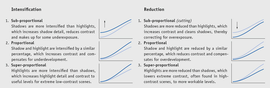
fig.15     Negatives are stored in oxidantand acid-free sleeves, which are properly labeled for future reference. It is convenient to file copy sheets and printing records together with the negative sleeves.

Negative Storage

Negatives usually have a good chance to survive the challenges of time, because they are often well protected, handled rarely and stored in the dark. However, common reasons for negatives to have a reduced life expectancy are sloppy film processing, ill handling, unnecessary exposure to light, extreme humidity, inappropriate storage materials and adverse environmental conditions. A summary of important film processing, handling and negative storage recommendations are in the text box below. These recommendations are not as strict as a museum or national archive would demand, but they are practical and robust enough to protect valuable negatives for a long time. Reasonable care will go a long way towards the longevity of photographic materials.

The main message I want you to take away from the last two chapters is that we use exposure to control the shadow densities of the negative, and we use development control to achieve the appropriate highlight densities. This balance between exposure and development control will create a negative that is easy to print, and it also promotes print manipulation from salvaging technique to creative freedom.

 

Advanced Development

Are one film and one developer enough?

It is prudent to evaluate the effect of developers and film processing variables on negative quality, to verify if one can sufficiently alter a film’s characteristics to suit universal or specific applications. In previous chapters, we have only discussed changing the film development time to accommodate the subject brightness range. We have not explored the consequences to negative characteristics, other than contrast, or the creative opportunities obtained from changing the developer or processing technique. This is especially interesting when one considers the claims made for various old developers not knowing how they affect modern films. The subject is vast, and over the years, most photographic books have touched on the subject. Two Focal Press publications stand out, Developing by Jacobson & Jacobson and The Film Developing Cookbook, by Anchell & Troop. However, even these books do not compare the variation in speed, grain, resolution and sharpness obtainable from one film by changing the developer or processing technique.

In this chapter, we can only scratch the surface and compare the results obtainable with one film and one standard developer with the results obtained with two other commonly used developers. The findings presented here infer, but do not assure, that a similar trend will exist with other emulsions and developers.

A major driver to improve film and developer materials has been the need to extract maximum quality (fine grain and high speed, sharpness and resolution) from small negative formats for the purpose of high-magnification enlargements. These attributes are less critical at the lower magnifications required with medium and large film formats. Assuming that fine-art photographers will predominantly use medium-format or larger negative sizes, this study employs a 6x7 roll film camera with a lens of proven high contrast and resolution, loaded with a medium-speed film. In addition, a pictorial comparison is made with print enlargements made from highly magnified 35mm negatives to examine the grain and edge effects.

Outline

The objective of the first part of this evaluation is to compare the effects on tonality, grain, speed, sharpness and resolution obtainable from one film and one developer (Ilford HP5 Plus and ID-11), by varying the agitation and dilution of the development process. HP5 and ID-11 are representative of standard materials and should be indicative of other standards, such as Kodak Tri-X and D-76. The second part of the evaluation compares the range of results obtained from this combination, by substituting ID-11 with Ilford Perceptol (Microdol-X) and Agfa Rodinal, as prime examples of fine-grain and high-acutance developers, at normal dilutions and with intermittent agitation. In each case, the development time was adjusted to ensure normal negative contrast (N).

Parameter Setting

An initial evaluation at fixed developer dilution and agitation, with development temperature set to 18°C and 24°C, and the development time adjusted to give normal contrast, yielded indistinguishable negatives. A literature search confirmed the potential effects of dilution and agitation on tonality, grain, speed, sharpness and resolution, but there were few mentions of temperature related effects. As a result, only developer dilution and agitation were considered significant process variables that affect negative characteristics and the final print.

fig.1       Most active developing agents are based on benzine rings. The active ingredients shown here are represented in the three developers that are compared in this chapter. ID-11 (D-76) uses a combination of Metol and Hydroquinone, Rodinal uses para-aminophenol and Perceptol (Microdol-X) uses Metol alone.

The required developer dilution is highly dependent upon the actual developer used. Agfa Rodinal, for example, has standard dilutions of 1+25 and 1+50 but can be used up to 1+200. ID-11 is typically used undiluted, 1+1 and 1+3. At higher dilutions, there may be a lack of active developing agents in the solution to fully develop the film. This evaluation uses two dilutions (1+1 and 1+3) and the two extremes of agitation (continuous and stand), using a Jobo CPE-2 rotary processor and standard development tanks.

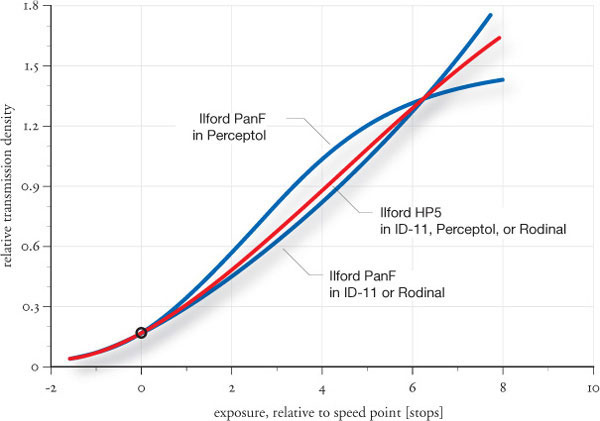
fig.2       A comparison of PanF and HP5 characteristic curves, developed in three different developers, demonstrates the uniqueness of certain combinations. HP5 characteristics are almost identical with all three developers, whereas PanF responds differently to one developer. This highlights the potential error of generalizing developer properties and reinforces the point that the only way to really understand material behavior is to test it.

Calibration

A serious exposure or development error can significantly change negative grain and resolution. A meaningful comparison mandates that negatives with identical effective exposure and contrast are made. Consequently, initial testing was required to establish a standard development time and the exposure index (EI) for each film, developer and all agitation and dilution combinations in question. For this, a Stouffer step tablet was photographed repeatedly to create a sufficient amount of test films. These films were subsequently processed, according to a test plan, which included all developers and developing schemes.

After drying, the films were evaluated, using the process laid out in the chapter ‘Creating a Standard’, and the speed points and gradients were measured. This employed the ‘Film Average Gradient Meter’ and ‘Film Characteristic Curves’ found in the ‘Tables and Templates’ section to establish the normal development time and the effective film exposure index for each variation. At this point, I was able to compare the relative exposure indexes for each combination.

fig.3       Film selection is always a compromise between film speed, sharpness and resolution. No film can have it all!

Pictorial Analysis

I also conducted a pictorial analysis to compare tonality, grain, sharpness and resolution, by using resolution and MTF targets and evaluating the pictorial impact on a detailed high-contrast scene. Using the predetermined EI and development times for each development scheme, eight films were exposed at the effective EI, carefully labeled, developed and their negatives enlarged to make prints.

For each film, the resolution values at which the MTF contrast fell to 50% and 10% of its peak were obtained, using the measurement methods established in the chapter ‘Digital Capture Alternatives’. These give an objective indicator of acceptable sharpness and resolution, respectively. The prints give a pictorial presentation of grain and acutance. These are enlarged sufficiently to overcome the limitations of the book printing process and should be viewed at arm’s length to mimic a more realistic reproduction ratio.

Results

Tonality

Some emulsion and developer combinations are known for their individual characteristics. In this particular instance, Ilford HP5 in Perceptol, Rodinal and the various ID-11 combinations give a consistent, almost straight-line characteristic curve with a slight toe and no shoulder. Fig.2 shows a typical characteristic curve for HP5 in any of these three developers. From previous experience, I know that ID-11 and Perceptol can behave very differently with other films. Fig.2 also compares the tonality of Ilford HP5 and PanF in ID-11, Rodinal and Perceptol. Clearly, there are hidden synergies with certain film and developer combinations, which can only be obtained with patient experimentation.

Speed

An exposure index or speed variation of 2/3 stop was achieved by changing ID-11’s concentration and the agitation scheme. The developers Rodinal and Perceptol create lower exposure indexes. High-dilution, stand development yielded the highest exposure index, and low-dilution, continuous-agitation development, created the lowest. In general, with one developer, the longer the development time, the higher the exposure index, for the same negative contrast.

Sharpness and Resolution

As well as the stable tonality of HP5 in the three developers, resolution was largely unaffected by the various ID-11 development schemes or by changing the developer. The resolution measurements are statistically the same for all the combinations. In all cases, the resolution on medium-format film is sufficient for standard viewing conditions, and in most cases, better than required for critical viewing conditions.

A literature search suggests that high-dilution and low-agitation development enhance sharpness through image edge effects or acutance. Coarser details, measured at the 50% MTF point, showed the slightest increase in contrast for the dilute, low-agitation combination. Rodinal, known for its sharpness, fared no better than dilute ID-11 with stand development.

Grain

A quantitative grain measurement is impractical for the amateur, but one can see and compare its effect and intrusion in enlargements. For this evaluation, a detailed high-contrast scene was photographed on 35mm HP5 with a particularly high-resolution, Carl Zeiss Distagon 2/35 ZF, lens on a Nikon F3. The scene was captured repeatedly at constant aperture and with bracketed exposure sequences. The film was cut into short sections and developed according to the predetermined schemes. Print enlargements with 20x magnification were made from equivalently exposed negatives (see fig.6), showing the pictorial impact of tonality, grain, sharpness and resolution.

The prints from negatives developed in ID-11 were virtually identical, apart from a slight improvement to fine tracery in the pylon and branches, a slightly lower local contrast between light and dark areas, and more even grain in the film developed with continuous agitation. There were no detectable edge effects in the continuous or stand-developed negatives. Prints made from negatives developed in Perceptol were similar, but they had slightly softer grain, which is in stark contrast to those developed in Rodinal.

Agfa’s Rodinal, it’s fair to say, is in a class of its own. With HP5, it produced negatives with character, giving detail to every faint twig, leaf and strut from the negative and adding an etched appearance to the image. The grain is very well defined and appears coarser than in the other prints. It is a classic case of a grain trade-off against increased visual sharpness.

Are one film and one developer enough?

Over the years, I have used many film, developer and process combinations. Fueled with this experience and the claims of other publications, I approached this study with the expectation of a revelation. Even after numerous tests and calibrations, I scratched only the surface of this vast subject, yet found a significant outcome. It would appear that, since the days of Ansel Adams, the film companies have made their products more robust to processing variables.

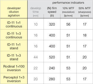
fig.4       This comparison shows that HP5 is very robust to different developers, dilutions and agitation techniques. The most obvious difference between development schemes is the effective film speed. Also, higher dilutions of ID-11 provide more sharpness (50% MTF), similar to the high-sharpness developer Rodinal. However, at print sizes of 16x20 or smaller, these differences are hardly recognizable with medium or large-format negatives. With 35mm film, on the other hand, resolution and sharpness differences become more obvious, due to the increased enlargement factor (see fig.6).

Contrary to expectation, only subtle changes, unlikely to be visible at moderate enlargements, could be achieved by changing ID-11 dilution and agitation with HP5, mostly in apparent sharpness and film speed. Changing the developer had a more profound effect on speed, sharpness and grain. Tonality was unaffected, but as identified by prior observations with Ilford PanF, tonality is specific to a particular combination of developer and emulsion. While some developers, such as Rodinal, have a definite character that imposes itself on whatever it develops, many others are more middle-of-the-road developers. The inability to reliably predict the relative characteristics of most developer and emulsion combinations may well be the reason for the lack of such information in other publications.

Apparently, one film and one developer are not enough to meet all needs. One requires a few films, which cover a range of applications, as well as an all-purpose standard developer, such as D-76 or ID-11. The resulting combinations should be used with a consistent development process. For special applications, which require specific visual attributes, one should select an alternate developer, proven by experiment, to give the desired visual affect.

fig.5       A graphical presentation of the data in fig.4 illustrates the limitations of Ilford’s HP5’s response to different developers and developing techniques.

And yet, photographic chemistry rumors will most likely live on, despite scientific evaluation to the contrary. For instance, I decided to find out what was behind the miraculous claims attributed to prints made from stained negatives, which are created with Pyrogallol and Pyrocatechol developing agents in combination with Metol. These claims include improved grain, acutance and unmatched highlight separation. Although these developers have a reputation for being sensitive to aging, agitation, oxidation and streaking, they have a strong following and continuously draw interest with people who, for whatever reason, are not satisfied with established products. My own sensitometry study and subjective comparison of three staining developers with a Metol-only developer (Perceptol) on HP5 produced four indistinguishable prints, despite these claims. In other words, at least in case of Ilford HP5 Plus, the claims are completely unjustified. Even so, the allure of the super-developer, solving all issues, remains undiminished, and it will take some time for some users to realize that the latest formula is just ‘another’ developer and not a magic recipe. It is important to realize that the robustness of an established developer, like Ilford’s ID-11, Kodak’s D-76 and Agfa’s Rodinal, which have been around for many decades, is often more important than fickle formulae with minor pictorial gain. Only adhering to robust darkroom processes and stabilizing one’s own technique, while establishing a thorough understanding of material behavior and responses, assures the results we all seek to be proud of.

fig.6a    ID-11, 1+1, continuous agitation

fig.6b    ID-11, 1+3, stand agitation

fig.6c    Rodinal, 1+100, intermittent agitation

fig.6d    Perceptol, 1+3, intermittent agitation

fig.6       These 20x enlargements of HP5 negatives indicate the extremes achieved with different developers, dilutions and agitation techniques. They show what I was unable to differentiate analytically. In fig.6a, ID-11 1+1 and continuous agitation brings out the fine details of the pylon and tree, but the lack of sharpness loses the visibility of some tracery. In fig.6b, ID-11 1+3 and stand development increases sharpness in fine details and local contrast but at the danger of obliterating the finest details with coarser grain. Some of the details look etched away. This trend is taken to extreme in fig.6c, where Rodinal and intermittent agitation accentuates the details in branches and pylon structure. Remarkably, this achieves a similar resolution as with ID-11 but with an obvious increase in grain. In fig.6d, Perceptol 1+3 and intermittent agitation produces the smoothest grain of all tested development schemes with otherwise similar properties to ID-11 1+1 with continuous agitation.

Creating a Standard

Tone reproduction defines the boundaries and target values of the Zone System

A fine print can only come from a quality negative, and the Zone System is a fantastic tool to create such a perfect negative. Over the years, many Zone System practitioners have modified what they had been taught, adjusting the system to fit their own needs and work habits. This flexibility for customization has left some photographers with the perception that there are many different Zone Systems. That is not the case, but different interpretations and definitions of some key target values and boundary conditions do indeed exist. It is, therefore, beneficial for the rest of the book and the reader’s understanding to create a ‘standard’ for some of the exposure and development assumptions, when using the Zone System. This will help to create a consistent message, eliminate confusion and build a solid foundation for your own customization in the future.

Reading Shadows and Highlights

Expose for the shadows. This means that you have to select a shadow area, read the reflected light value with your spotmeter and then place it onto the appropriate zone to determine the exposure. This process is very subjective, because the appropriate zone is found through visualization alone. You find photographers using any one of Zone II, III or IV as a base for the shadow reading. Ansel Adams suggested Zone III, due to the fact that it still has textured shadows with important detail. Zone III creates a fairly obvious boundary between the fully textured details of Zone IV and the mere shadow tonality of Zone II. My experience shows that Zone IV is often selected with less confidence and consistency, and Zone II reflects only about 2% light, making accurate readings challenging for some equipment. Consequently, we will standardize on Zone III as the basis to determine shadow exposure.

Develop for the highlights. This means that you have to select a highlight area, read the reflected light value with your spotmeter and determine what zone it ‘fell’ onto. If that is not the visualized zone, then development correction is required to get it there. To standardize on this zone for highlights is not simple, because it depends entirely on the subject. It could be a Zone V in a low-key image and it could be a Zone XI in the highlights of a snow filled scene. However, most of these situations are special cases, and we can safely assume that we will standardize on a scene with a complete tonal range from black to white. Ansel Adams suggested Zone VII, due to the fact that it still has textured highlights with important detail. Many beginners are surprised how ‘dark’ Zone VII is, and it seems to be far easier to visualize a Zone VIII, where we still find the brightest important highlights, before they quickly disappear into the last faint signs of tonality and then into paper white. We will standardize on Zone VIII as a basis to determine film development.

Practical Boundaries

We have to remind ourselves that, in analog photography, the print is the only means of communication with the viewer of our photographs. Therefore, negative density boundaries have to support, and are limited by, the paper density boundaries. They have been defined in ‘Tone Reproduction’ and will be covered further in ‘Fine-Tuning Print Exposure and Contrast’. We know from both chapters that modern printing papers are capable of representing 7 zones under normal lighting conditions. We will standardize on a normal subject brightness range to have 7 zones from the beginning of Zone II to the end of Zone VIII with relative log transmission densities of 0.17 and 1.37, respectively. These values assume the use of a diffusion enlarger and need adjustment if a condenser enlarger is used. Consequently, our standard negative density range is 1.20.

The log exposure range of grade-2 paper is limited to 1.05, but this ignores extreme low and high reflection densities. We have no problem fitting a negative density range of 1.20 onto grade-2 paper, if we allow the low end of Zone II and the high end of VIII to occupy these paper extremes. Our standard paper contrast is ISO grade 2.

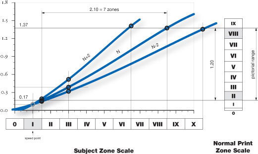
fig.1a    Setting the speed point at Zone I allows for some fluctuations in low shadows (Zone I·5), and N-2 development leads to slightly weak shadow densities.

fig.1a    With the speed point at Zone III, low shadow densities are inconsistent and far too weak with N+2 development. Highlights fluctuate by about one paper zone.

fig.1c    Setting the speed point at Zone I·5 secures consistent densities for shadow and highlight tones regardless of development compensation. It is best to always place the speed point at the shadow anchor of the Zone System.

A simple definition for compensating development is also required. Despite some existing textbooks with rather complicated definitions, we will use a very simple but useful interpretation. As stated above, normal development (N) will capture 7 zones (2.10 log exposure) within the fixed negative density range. N-1 will capture one zone more with reduced development, and N+1 will capture one zone less with increased development. A complete list can be seen in the bottom half of fig.2.

Speed Point

We saw in the chapter ‘Development and Film Processing’ how the development time changes the average gradient and how it allows us to compensate for different lighting situations. Shorter development captures more subject brightness zones in a fixed negative density range, and longer development has the opposite effect. Of course, we are doing so to keep almost all maximum negative density at a fixed level, allowing all lighting scenarios to be printed on grade 2 paper. This leaves us with maximum paper contrast control and creative flexibility. In a dull low-contrast scene, the contrast is increased, and in a high-contrast scene, the contrast is reduced. In the dull scene, Zone VI might be the brightest subject ‘highlight’, and the increased contrast will lift it to a density level typically reserved for Zone VIII. In a high-contrast scene, Zone X might be reduced to a Zone VIII density, to keep it from burning-out in the print.

The entire negative zone scale is affected when highlight density is controlled by development. The individual zone densities ‘move’ within their proportional relationship. However, we can select one common point for all development curves by controlling the film exposure. They will all intersect at this point, and all curves will have the same negative density for a specific subject zone. This point is called the ‘speed point’, because it is controlled by the film exposure in general and the film speed in particular. It is also often referred to as the ‘foot speed’, because it is most likely found near the toe of the characteristic curve, where exposure has more influence on negative density than development time.

It is up to us where to set the speed point on the subject zone scale, but some locations are better than others. Fig.1 illustrates some possible locations. In fig.1a, the speed point is located at Zone I. This is a popular choice, but it allows for some density fluctuations in low shadows around Zone I·5, and N-2 development leads to slightly weak shadow densities. Highlight densities are fairly consistent and the density variations for Zone III are of little concern. In fig.1b, the speed point is located at Zone III. This seems to be an obvious choice at first, because it secures consistent Zone III densities. However, the low shadow densities are highly inconsistent and far too weak with N+2 development. The highlight densities fluctuate by about one paper zone. In fig.1c, the speed point is located at Zone I·5. This secures consistent densities for shadow and highlight tones regardless of development compensation. The textural density variations for Zone III are less than 1/3 stop, which is unavoidable and of no concern. It is best to always place the speed point at the shadow anchor of the Zone System. For us this means that our standard speed point is at Zone I·5 and has a negative density of 0.17.

Average Gradient

The relationship between subject brightness range and average gradient in the Zone System can be taken from the two graphs in fig.2. This relationship is fixed to the Zone System development-compensations values if our standard values are assumed. In the subject-brightness-range graph (top), the normal scene is assumed to have a 7-stop difference between shadows and highlights. The average-gradient graph (bottom) is based on a fixed negative density range of 1.20. This negative density range assumes the use of a diffusion enlarger and an ISO grade-2 paper contrast as a desirable aim. You may want to lower the average gradient if you are working with a condenser enlarger. Their optics make a negative seem to be about a grade harder, but print with the same quality once the negative density range is adjusted. Use a negative density range of 0.90 as a starting point for your own evaluations. You may also want to make other adjustments to target average gradient values if you have severe lens and camera flare, or if you experience extremely low flare. The nomograph in ‘Customizing Film Speed and Development’ will help with any necessary adjustments.

We now have standard Zone System boundaries and target values. They can be used as a guide or as a rule, and they work well in practical photography. More importantly, we are using them throughout the book to be consistent.

fig.2       Subject brightness range (SBR) and average gradient (γ) have a fixed relationship to the Zone System development compensations when a few assumptions are made. In the subject-brightness-range graph (top), the normal scene is assumed to have a 7-stop difference between shadows and highlights. The average-gradient graph (bottom) is based on a fixed negative density range.

 

Customizing Film Speed and Development

Take control and make the Zone System work for you

Film manufacturers have spent a lot of time and resources establishing the film speed and the development time suggestions for their products. Not knowing the exact combination of products we use for our photographic intent, they have had to make a few assumptions. These assumptions have led to an agreement among film manufacturers, which were published as a standard in ASA PH2.5-1960. It was the first standard to gain worldwide acceptance, but it went through several revisions and was eventually replaced by the current standard ISO 6:1993, which combines the old ASA geometric sequence (50, 64, 80, 100, 125, 160, 200, …) with the old DIN log sequence (18, 19, 20, 21, 22, 23, 24, …). As an example, an ISO speed is written as ISO 100/21°.

Fig.2 shows a brief overview of the ISO standard. According to the standard, the film is exposed and processed so that a given log exposure of 1.30 has developed to a transmission density of 0.80, resulting in an average negative gradient of about 0.615. Then, the film speed is determined by the exposure, which is developed to a shadow density of 0.10. This makes it an acceptable standard for general photography. However, the standard’s assumptions may not be valid for every photographic subject matter, and advertised film speeds and development times can only be used as starting points.

A fine-art photographer appreciates fine shadow detail and often has to deal with subject brightness ranges that are significantly smaller or greater than the normal 7 stops from the beginning of Zone II to the end of Zone VIII. In addition, the use of certain equipment, like the type of enlarger or the amount of lens flare, influences the appropriate average gradient and final film speed. The nomograph in fig.14 gives an overview of these variables and their influence. The Zone System is designed to control all these variables through the proper exposure and development of the film. This requires adjustment of the manufacturer’s film speed (or ‘box speed’) and development suggestions.

In general, advertised ISO film speeds are too optimistic and suggested development times are too long. It is more appropriate to establish an ‘effective film speed’ and a customized development time, which are personalized to the photographer’s materials and technique. In most literature, the effective film speed is referred to as the exposure index (EI). Exposure index was a term used in older versions of the standard to describe a safety factor, but it was dropped with the standard update of 1960. Nevertheless, the term ‘EI’ is widely used when referring to the effective film speed, and we will accept the convention.

Still, we ask ourselves: How does one establish the effective film speed and development time to compensate for different subject brightness ranges?An organized test sequence can give you very accurate results, but even a few basic guidelines can make a big difference in picture quality. I would like to show you three different ways, with increasing amount of effort, to keep you from wasting your time on too many ‘trial and error’ methods.

1. Quick and Easy

Here is a simple technique, which will improve picture quality significantly and does not require any testing at all. Use it if you dislike testing with a passion, or if you just don’t have the time for a test at the moment. This method can also be used to give a new film a test drive and compare it to the one you are using now.

For a normal contrast, bright but cloudy day, cut the manufacturer’s recommended film speed by 2/3 stop (i.e. ISO 400/27° becomes ISO 250/25°) and the recommended development time by 15%. The increased exposure will boost the shadow detail, and the reduced development time will prevent the highlights from becoming too dense. For a high-contrast, bright and sunny day, increase the exposure by an additional 2/3 stop (i.e., ISO 400/27° now becomes ISO 160/23°) and reduce the development time by a total of 30%. Stick to the ‘box speed’ and suggested development time for images taken on a low-contrast, rainy or foggy day.

A negative processed this way will easily print with a diffusion enlarger on grade-2 or 2.5 papers. Just give it a try (fig.1). It is really that simple to make a significant improvement to negative and image quality.

2. Fast and Practical

Here is another way to arrive at your effective film speed and customized development time. It is a very practical approach, which considers the entire image producing process from film exposure to the final print. The results are more accurate than from the previous method, and it requires three simple tests, but no special equipment.

fig.1       It is possible to make significant improvements to negative and image quality without any testing. Use this table to deviate from the manufacture’s recommendations for film exposure and development according to overall scene contrast.

a. Paper-Black Density Test

This test will define the minimum print exposure required to produce a near-maximum paper density. Make sure to use a blank negative from a fully processed film of the same brand as to be tested. Add a scratch or a mark to it, and use it later as a focus aid.

1.   Insert the blank negative into the negative carrier.

2.   Set the enlarger height to project a full-frame 8x10 inch print and insert contrast filter 2 or equivalent.

3.   Focus accurately, then measure and record the distance from the easel to the film.

4.   Stop the lens down by 3 stops and record the f/stop.

5.   Prepare a test strip with 8, 10, 13, 16, 20, 25 and 32-second exposures.

6.   Process and dry normally.

fig.2       Film exposure and development in accordance with the current ISO standard.

7.   In normal room light, make sure that you have at least two but not more than five exposures, which are so dark that they barely differ from one another. Otherwise, go back to step (5) and make the necessary exposure corrections.

8.   Pick out the first two steps that barely differ from one another and select the lighter of the two.

9.   Record the exposure time for this step.

This is the exposure time required to reach a near-maximum paper density (Zone 0) for this aperture and magnification. If you can, leave the setup in place as it is, but record the f/stop, enlarger height and exposure time for future reference.

b. Effective Film Speed Test

This test will define your normal effective film speed, based on proper shadow exposure.

1.   Select a subject, which is rich in detailed shadows (Zone III) and has some shadow tonality (Zone II).

2.   Set your lightmeter to the advertised film speed.

3.   Stop the lens down 4 stops from wide open, and determine the exposure time for this aperture, either with an incident meter pointing to the camera, or place a ‘Kodak Gray Card’ into the scene, and take the reading with a spotmeter. Keep the exposure time within 1/8 and 1/250 of a second or modify the aperture.

4.   Make the first exposure.

5.   Open the lens aperture or change the ISO setting of your lightmeter to increase the exposure by 1/3 stop (i.e., ISO 400/27° becomes ISO 320/26°) and make another exposure. Record the exposure setting.

6.   Repeat step (5) four times, and then, fill the roll with the setting from step (4).

7.   Develop the film for 15% less time than recommended by the manufacturer. Otherwise, process and dry the film normally.

8.   Set your enlarger and timer to the recorded settings for the already determined Zone-0 exposure from the previous test.

9.   Print the first five frames, process and dry normally.

An evaluation of the prints will reveal how the shadow detail is improving rapidly with increased film exposure. However, there will come a point where increased exposure offers little further benefit. Select the first print with good shadow detail. The film speed used to expose the related negative is your normal effective film speed for this film. Based on my experience, it is normal for the effective film speed to be up to a stop slower than the rated film speed.

Fig.3a-c show just how much difference the effective film speed can make. Fig.3a is the result of a negative exposed at ISO 125/22° and then printed with the minimum exposure time required to get a Zone-0 film rebate with a grade-2 paper. The highlights are ‘dirty’, the midtones are too dark and ‘muddy’, and the shadows are ‘dead’ with little or no detail. In fig.3b, an attempt was made to produce a ‘best print’ from the same negative. The film rebate was ignored, the exposure was corrected for the highlights, and contrast was raised to optimize shadow appearance. The highlights and midtones are much improved, but the gray card is still a bit dark. The shadows are solid black, still without any detail, and the picture has an overall harsh look to it. Fig.3c is the result of a negative exposed at an effective film speed of EI 80, and then printed in the same way as fig.3a. The highlights are bright, but not as harsh as in fig.3b, the gray card is on Zone V as intended, and the shadows are deep black with detail. A big improvement, solely due to selecting the effective film speed.

c. Film Developing Time Test

This test will define your normal film development time. A rule of thumb will be used to adjust the normal development time to actual lighting condition, where needed.

1.   Take two rolls of film. Load one into the camera. On a cloudy but bright day, find a scene that has both significant shadow and highlight detail. A house with dark shrubs in the front yard and a white garage door is ideal.

2.   Secure your camera on a tripod, and set your lightmeter to your effective film speed, determined by the previous test. Meter the shadow detail, and place it on Zone III by reducing the measured exposure by 2 stops.

3.   At that setting, shoot the scene repeatedly until you have finished both rolls of film.

4.   In the darkroom cut both rolls in half. Develop one half roll at the manufacturer’s recommended time. Develop another half roll at the above time minus 15% and another half roll at minus 30%. Save the final half roll for fine-tuning.

5.   When the film is dry, make an 8x10-inch print from one negative of each piece of film at the Zone-0 exposure setting, determined during the first test. The developing time used to create the negative, producing the best highlight detail, is your normal film developing time. You may need the fourth half roll to fine-tune the development.

Considering your entire image-making equipment, you have now determined your effective film speed, producing optimum shadow detail, and your customized film developing time, producing the best printable highlight detail for normal lighting conditions.

However, film exposure and development have to be modified if lighting conditions deviate from ‘normal’. The rule of thumb is to increase the exposure by 1/3 stop whenever the subject brightness range is increased by one zone (N-1), while also decreasing development time by 15%. On the other hand, decrease the exposure by 1/3 stop whenever the subject brightness range is decreased by one zone (N+1), while increasing development time by 25%.

These tests must be conducted for every combination of film and developer you intend to use. Fortunately, this is not a lot of work and will make a world of difference in your photography.

3. Elaborate and Precise

The following method of determining the effective film speed and development time is more involved than the previous two, and it requires the help of a densitometer to read negative transmission densities accurately. The benefit, however, is that it supplies us will all the information we need within one test. It gives enough data to get the effective film speed and how it changes with different development times. We will also get an accurate development time for every possible subject brightness range. Negatives exposed and developed with this information should have a constant and predictable negative density range for any lighting situation. This method is ideally suited for use with the Zone System. The final results are well worth the time commitment of about 8 hours to perform the test and to evaluate the data.

fig.3a    The negative was exposed at ISO 125/22° and then printed with the minimum exposure time required to get a Zone-0 film rebate with a grade-2 paper. This results in ‘dirty’ highlights, ‘muddy’ midtones and ‘dead’ shadows.

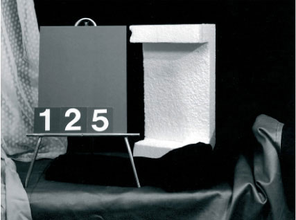
fig.3b    ISO 125/22°. Print exposure and contrast were changed to make ‘best print’. Highlights and midtones are improved, but there is still no shadow detail.

fig.3c    EI 80/18°. A film exposure increase but a print exposure as in fig.3a results in bright highlights similar to fig.3b, with improved midtone and shadow detail.

(test & images by Bernard Turnbull)

The use of a densitometer is essential for this test. A densitometer is costly and, therefore, typically a rare piece of equipment in regular darkrooms. A quality densitometer costs as much as a 35mm SLR, if purchased new, but they are often available for a fraction of that on the used market. This test only requires us to read transmission densities, but a densitometer which is able to read both transmission and reflection is a much more versatile piece of equipment. Some darkroom analyzers have a built-in densitometer function, and they can be used to read projected negative densities. Alternatively, you may ask a friend or the local photo lab to read the densities for you. Once you have a densitometer, you will find many uses for it around your darkroom.

Exposure

Many different methods of generating the necessary negative test exposures have been published. Most require changes to lens aperture or camera shutter settings for exposure control. If conducted with care, this is a very practical method providing acceptable accuracy. However, years of testing have made me aware of some equipment limitations, which we need to take into consideration to get reliable results.

Mechanical shutters are rarely within 1/3-stop accuracy, and their performance is very temperature sensitive, acting slower when cold. They also become sluggish after long periods of non-use. In these cases, it helps to work the shutter by triggering the mechanism a few times. In any event, they cannot be set in fine increments, and exposure deviations should be recorded down to 1/3 stop. This is not possible with mechanical shutters. Electronic shutters, on the other hand, are very precise, and sometimes provide 1/3-stop increments, although they are uncommon in large-format equipment. Lens aperture accuracy is usually very good, being within 1/10 stop, but apertures are notorious for being off at the largest and smallest setting. Medium aperture settings are far more trustworthy, but only if worked in one direction. Switching from f/8 to f/11 may not result in the same aperture as switching from f/16 to f/11, due to what is known as mechanical hysteresis. Consequently, we can use shutters and lens apertures to control test exposures, but must avoid mechanical shutters and change f/stops only in one direction.

fig.4       The Stouffer 31-step tablet

As an alternative, consider the use of a step tablet wherever possible. A step tablet is a very accurate and repeatable way to expose a piece of film. Fig.4 shows one supplied by Stouffer in Indiana, but they are available from different manufactures and in different sizes. The process is most simple if you purchase one in the same size as the negative format to be tested, and photograph it with the aid of a slide duplicator. If such a device is not available, then a similar setup can easily be rigged up. It can be as simple as placing the step tablet onto a light table, and taking a close-up copy.

I prefer the 31-step tablet to the 21-step version, due to the higher quantity of data points available. However, in the process of copying the step tablet, be certain that the steps on the final negative are wider than the measuring cell of the densitometer, otherwise you will not be able to read the density values properly. This may necessitate opting for the 21-step version with its wider bars or adjusting the scaling when you photograph the step tablet. This will be most likely the case only with 35mm negatives. You should be able to fit the 31-step version with most medium format and 4x5-inch film.

Film has a different sensitivity to different wavelengths of light. Therefore, select a light source with a color temperature representative of your typical subject matter and setup. In other words, use daylight or daylight bulbs if you are a landscape photographer, and use photofloods or flashlight if you mainly work in the studio. However, always keep exposure times between 1/500 s and 1/2 s to avoid reciprocity failure.

Assume the box speed to be correct and determine the right exposure with an average reading, or use a spotmeter for the medium gray bars. You can use the manufacturer’s recommended film speed, since the actual exposure is not critical as long as it is within 1 stop. The worst that can happen is that a few bars are lost on either end. Once the step tablet is photographed and developed, you will have 21 or 31 accurately spaced exposures on every frame. They are accurate, because their relative exposure is fixed through the densities of the step tablet, and are not affected by any shutter speed or lens aperture inaccuracies. If you are testing sheet film, expose five sheets with the same exposure. If you are testing roll film, fill five rolls of film with the same exposure on every frame.

Development

Select the developer, its dilution and temperature you intend to use for this film. Develop the film in the same manner as you would normally, but for fixed and closely controlled development times. Develop the first roll or sheet for 4 minutes, the next for 5.5 minutes and the following for 8, 11 and 16 minutes, respectively. Start timing after the developer has been poured into the developing tank, and stop timing after it has been poured out again. Process and dry all film normally.

Make sure that all processing variables are constant and the only difference between these films is the development time. The temperature of the developer is critical, but it is more important to have a consistent temperature than an accurate one. Try to maintain an almost constant developer temperature throughout the process. Keeping the developing tank in a tempered water bath will help to do so. It does not matter if your thermometer is off by a degree or two as long as it reads the same temperature for the same amount of heat all the time. Do not switch thermometers. Pick one, and stick to it for all of your darkroom calibrations. For this test, all chemicals should be used as one-shot, but most importantly, do not reuse any developer solution. It does exhaust with use, and these five films must be developed consistently. The other chemicals are not as critical, but I still suggest using fresh chemicals for film development.

In addition, watch the film/developer ratio. The active ingredients of the developer are gradually exhausted during development. The rate of exhaustion during the test must be similar to your typical application. For example, do not develop one 4x5 test sheet in 1.5 liters of developer if you normally process six at a time in the same volume. Six sheets of film will exhaust the developer more quickly than just one, and consequently, negative densities of the test film will be higher than from normal development. In this case, prepare additional test sheets, also exposed with the step tablet, and develop them together with the actual test film.

Always conduct the test with film in your favored format. Emulsion thicknesses differ between film formats, and consequently, so does the development time. A test based on one film format may not be valid for another.

Collecting and Charting the Data

As previously mentioned, a transmission densitometer is the appropriate tool to measure the test densities. It is best to prepare a spreadsheet with six columns: the first column for the step tablet densities and the others for the negative densities of the five test films. Ideally, the 21-step tablet should have 0.15 step-to-step density increments, and the 31-step tablet should have 0.1-density increments. Be aware that your step tablet will most likely deviate slightly from these anticipated values. This is also true for calibrated step tablets. Therefore, read the densities of the step tablet itself, and list them in the first column. The test results will be more precise when charting the test data against these actual values.

Read the densities of the five tests, and fill them into the spreadsheet. My densitometer has a calibration button to ‘zero’ out the measurements, because it does not have an internal light source of known intensity for transmission density readings. In other words, it can be used with different light sources and allows for relative and absolute density measurements. If your equipment has a similar feature, then take the first reading with nothing in the light path, push the ‘zero’ button, and then, continue to take all the measurements. This will enable you to measure the ‘base+fog’ density of the test negatives. If you ‘zero’ the measurements to a blank piece of the film before taking any readings, then all base+fog densities are equalized, and you would be unaware of any fog increase due to development time. If your densitometer does not have a ‘zero’ button, which is most likely the case if it has its own light source, then you can be assured that your readings are absolute values and no correction is required.

The typical measurement accuracy of a standard densitometer is ±0.02 density, with a reading repeatability of ±0.01 at best. This is a more than adequate measurement performance for a film development test. In addition, be aware that the Stouffer step tablet repeats step 16, and so we only need one reading for this density. Feel free to average the two readings if you find them to be slightly different.

fig.5       A ‘family of curves’ illustrates how the development time changes the negative transmission density.

fig.6       Film exposure and development have been adjusted to work in harmony with the Zone System. The speed point has been raised to a density of 0.17 to secure proper shadow exposure. In this example, the development has been adjusted to fit a normal subject brightness range of 7 zones into a fixed negative density range of 1.20, which is a normal range for diffusion enlargers and grade-2 paper. Development modifications will allow other lighting conditions to be accommodated for them to fit the same negative density range.

A spreadsheet is a good way to collect and view numerical data, but you need to graph individual tests in order to evaluate the results more closely. A blank form, to graph the test data, is included in the ‘Tables and Templates’ chapter at the end of the book. You may employ a computer for this task, however, it is important that you keep the same axis scales as the supplied graph. Otherwise, you will get false results from the overlays we are about to use. The relative log exposure is traditionally plotted on the horizontal axis and the transmission density is plotted on the vertical axis. The major ticks are in increments of 0.3 unit steps, which correlate conveniently with 1 stop of exposure. The family of curves will look similar to our example in fig.5 once the numerical data has been successfully transferred to the graph.

Evaluating the Data

With the aid of an overlay provided in ‘Tables and Templates’, you will have to take two types of measurement per curve, in order to evaluate the data (see fig.8). One is the average gradient, and the other is the relative log exposure of the speed point.

The average gradient is simply the ratio of the density range over the log exposure range. Film manufacturers and Zone System practitioners agree with the above definition of average gradient, but they differ when it comes to the selection of the boundaries for the calculation.

In fig.2, we saw how the ISO standard defines normal development as a log exposure range of 1.30 and a density range of 0.80, measured at a 0.10 shadow density. We will now replace these values with our Zone System target values as explained in ‘Creating a Standard’. Fig.6 illustrates the change, which will better suit the Zone System and fine-art photography. First, we use our minimum shadow and speed-point density of 0.17. This ensures proper shadow exposure, even when development time is reduced to support high-contrast scenes. Second, we use our standard fixed negative density range of 1.20 (pictorial range). This covers the entire paper exposure range, from the beginning of Zone II to the end of Zone VIII, for normal graded papers printed with a diffusion enlarger. This, combined with a minimum shadow density of Dmin = 0.17, fixes the maximum highlight density at Dmax = 1.37. In addition, it also sets the normal log exposure range to 2.10, since we need 7 subject brightness zones to expose the 7 paper zones above, and each zone is equivalent to 0.3 log exposure. The normal average gradient can be calculated as 1.20 / 2.10 = 0.57.

The ‘Tables and Templates’ chapter also includes an overlay called ‘Film Average Gradient Meter’, which is a handy evaluation tool based on our Zone System standard. The use of the ‘Film Average Gradient Meter’ overlay is shown in fig.7, as it is applied to the 8-minute development test. The other curves have been removed for clarity. The overlay is placed on top of the graph in a way that the ‘base+fog density’ line is parallel to the grid, but tangent to the toe of the curve. The overlay is then moved horizontally until the effective film speed for ‘Zone I·5 = 0.17’ intersects with the curve at the speed point. Fig.7 shows the overlay in this final position at which the reading can be taken. Take the average gradient reading as close to the ‘Zone VIII·5 = 1.37’ density as possible. In this example, 0.55 is the average gradient for the 8-minute curve. Before you move or put the template away, you need to measure the relative log exposure at the ‘effective film speed’ marker. In our example, 0.80 is the log exposure that created a minimum shadow density of 0.17. Record the average gradient and the relative log exposure in a table similar to the one shown in fig.8.

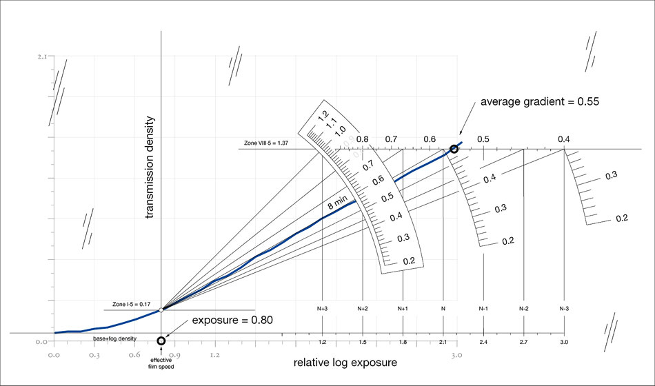
fig.7       As an example, the transparent ‘Film Average Gradient Meter’ overlay is used to measure the average gradient and the relative log exposure of the effective film speed for the 8-minute characteristic curve. This is done for all characteristic curves in fig.5 and the results are shown in fig.8.

Evaluate the rest of the test curves in the same way and record all readings. When finished, you will have a valuable table showing the entire test data.

Predicting Development Times

We are beginning to close the loop, and we are finally getting to chart some of the results, which will guide us to use our film effectively. The ability to precisely predict development times, in order to cope with many lighting scenarios, is a major advantage. We have now collected enough data to start filling out the ‘Film Test Summary’ template. Again, a blank form is included in ‘Tables and Templates’. It has four sections, and we will use them in sequence.

In fig.9a, the average gradient is plotted against the development time. We conducted five development tests, and therefore, we have five data points. Draw a point for every average gradient, which you measured with the ‘Film Average Gradient Meter’ for 4, 5.5, 8, 11 and 16 minutes of development time. In our example in fig.7, we measured an average gradient of 0.55 and that is where we draw a point on the 8-minute line. Now, draw a smooth curve through the data points. I use a computer to ‘curve fit’ the line, but there are other options. Feel free to create it freehand, use a bend ruler, or use a set of French Curves, available from any drafting supply store for a small outlay. The point is that you need an averaging line through the data points; how you get there is irrelevant. You see from fig.9b how this can help determine the appropriate development time for any average gradient.

The relationship between development compensations in Zone System ‘N’ terms and the average gradient was explained in ‘Creating a Standard’. Fig.10 shows the relationship in the form of a graph, a table and two equations. I used the values of the small table to mark the smooth curve in fig.9b at development expansion and contractions from N-2 to N+2. We can go a step further by plotting the ‘N’ values directly against the development times, as illustrated in fig.11. There is little difference to the previous graph, but the five average-gradient values from the test were first converted to ‘N’ values. To do that, either use the graph in fig.10 to estimate the closest ‘N’ value for each average gradient, or, if you are more comfortable with math, compute the ‘N’ value with the equation listed there. If you are comfortable thinking of development compensations in terms of N- or N+, you may find the graph in fig.11 more useful than the graph in fig.9b. Some people find this easier than thinking of target contrast in terms of average gradient. The result is the same; it is just presented in a different way.

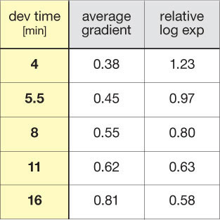
fig.8       The results from the development test in fig.5 are recorded in a table.

With these graphs at hand, predicting accurate development times has become simple. However, care must be taken not to alter any of the other significant variables. Be sure to keep temperature, chemical dilution, film/developer ratio and agitation as constant as possible.

fig.9a-b The average gradient for each test is first plotted, then a smooth curve fit is applied and the typical Zone System development compensations are marked for reference.

Predicting Effective Film Speeds

The final task is determining the effective film speeds for all developments. Of course, we would like to have these effective film speeds in ISO units, but doing this directly is a complex task and involves laboratory equipment not available to a fine-art photographer. The only data obtainable at this point are the relative log exposures required to develop the speed point densities as measured with the ‘Film Average Gradient Meter’ in fig.7. We will convert these relative log exposures to effective film speeds in a moment.

First, plot the test values from fig.8 in terms of average gradient versus relative log exposure of their effective film speeds, as shown in fig.12a, and draw a smooth line through the data points. Then, as shown in fig.12b, find the intersection of the N-development’s average gradient (0.57) and the curve. Project it down to the relative log exposure axis. There you will find the relative log exposure for an N-development (0.75), as marked with the gray circle. This log exposure is equivalent to the normal EI, which is the normal effective film speed for this film/developer combination. However, to get the normal EI in terms of ISO units, we must conduct one last test.

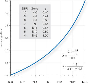
fig.10     Average gradient and Zone System compensations can be estimated or calculated. See ‘Creating a Standard’ for details.

1.   Use an evenly illuminated Kodak Gray Card as a test target (see fig.12c).

2.   Set your lightmeter to twice the advertised film speed and take a reading from the card.

3.   Place the reading on Zone I·5 and determine the exposure for an aperture closed down by 4 stops. Keep the exposure time within 1/8 and 1/125 of a second or modify the aperture.

4.   Make the first exposure.

5.   Open the lens aperture to increase the exposure by 1/3 stop, and make another exposure.

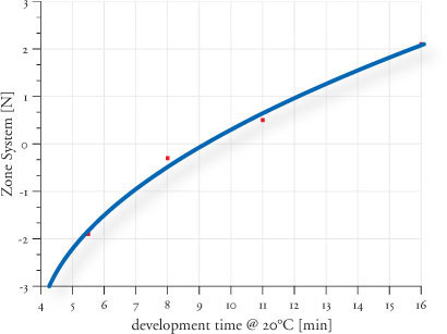
fig.11     A practical development chart is created, when the ‘N’ values are plotted against the development time.

6.   Repeat step (5) nine times to simulate different effective film speeds over a range of 3 stops in 1/3-stop increments, but don’t change the exposure time.

7.   With roll film, set your lightmeter back to the advertised film speed and expose the remaining frames with Zone-V exposures.

8.   Develop the film for the time established as a normal N-development in fig.11. Process and dry the film normally.

9.   Using a densitometer, start with the first frame and twice the box speed, count down 1/3 stop for every frame until you find the frame with a transmission density closest to a speed-point density of 0.17 (Zone I·5). The film speed used to expose this frame is your customized ‘normal EI’ (fig.12c).

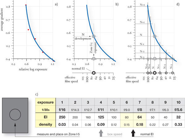
fig.12a  (top left) The test values from fig.8 are plotted in terms of average gradient versus relative log exposure, and a smooth curve is drawn through the data points.

fig.12b  (top center) Find the intersection of the average gradient for N and the curve. Project it down to the relative log exposure axis to find the relative log exposure for N.

fig.12c  Zone I·5-exposures in 1/3-stop increments are evaluated to determine the ISO speed for a normal EI. This is aligned with the relative log exposure in fig.12b.

fig.12d  (top right) More average-gradients values are projected onto the bottom axis to determine the missing film speeds for other Zone System developments.

We can relate the data from the curve in fig.12b to film speeds, because the relationship between log exposures and ISO speeds is known. A 0.1 log exposure difference is equal to a 1/3 stop difference in film speed. The effective film speed scale below the relative log exposure axis illustrates this relationship. It uses the normal EI as a starting point, and we are now ready to specify the effective film speed for any average gradient. In fig.12d, the typical values for N-3 to N+2 were projected on the curve and onto the log exposure axis, where they were marked with gray circles. Extending the projection to the effective film speed scale yields the EI for all development compensations this particular film/developer combination is capable of.

The graph must be cleaned up a bit so the data is readily available in the field. An improved graph is shown in fig.13. The ‘N’ values are plotted directly against the effective film speed. We can see how the film sensitivity decreases with development contraction. In other words, the film requires significantly more exposure to maintain constant shadow densities, when development time is reduced.

fig.13     This improved graph is a useful guide for Zone System exposures.

fig.14     This contrast control nomograph, based on a Kodak original, is designed to determine the appropriate average gradient and film exposure adjustment for different enlargers, lighting situations and camera flare. Select the required average gradient for your enlarger that gives a negative density range, fitting well on normal contrast paper. Draw a straight line through the subject brightness range and extend until it intersects with the adjusted average gradient. Draw another straight line through your typical camera flare value and extend it to find the final average gradient and the approximate exposure adjustment. One example is shown for a typical diffusion enlarger, a slightly soft (N+1) lighting condition and the use of an older, uncoated lens with very high flare. The average gradient is raised from 0.57 to 0.67 due to the lighting condition. The lens flare requires a further increase to 0.84, and exposure must be reduced by 1/2 stop.

Equipment Influence

You may want to lower the average gradient if you are working with a condenser enlarger. Their optics make a negative seem to be about a grade harder, but print with the same quality once the negative density range is adjusted. Use a fixed negative density range of 0.90 as a starting point for condenser enlargers. In addition, you may also want to make other adjustments to target average-gradient values if you have severe lens and camera flare, or if you experience extremely low flare. Fig.14 will help to approximate a target average gradient and exposure compensation, but I have not found any need to do so with any of my equipment.

Conclusion

A precise film-speed and development test is not a simple task. It requires some special equipment, some time, patience, practice and several non-photographic related skills. But the rewards are high. Fig.13 contains all information required to properly expose a given film under any lighting condition and then develop it in a given developer with the confidence to get quality negatives. These negatives will print well on a standard ISO grade-2 paper when using a diffusion enlarger. In my view, all the hard work has paid off. There is no need to worry about exposure and development anymore. No need to bracket exposures endlessly or to hope that it will ‘work out’. The occasional gremlin aside, it will. Now, all attention can be directed entirely towards the interaction of light and shadows, making and not taking a photograph, and therefore ultimately producing a piece of art.

Nevertheless, if this is all too much technical tinkering and you prefer to spend your time creating images, then remember that even a simplified method, as shown in ‘Quick and Easy’ or ‘Fast and Practical’, will improve negative and print quality significantly.

 

Influence of Exposure and Development

Expose for the shadows and develop for the highlights

Even with the best planning and testing, we are sometimes forced to work under less than perfect conditions. We thought we had loaded ISO 400/27° film, but actually, it was the left-over ISO 100/21° from the last model shoot, or we looked up the wrong time on our development table. Whether intentional or not, film exposure and development deviations have consequences, which must be fully understood to implement potential recovery methods and get the most from our negatives.

For more than a century, experienced photographers have advised us to expose for the shadows and to develop for the highlights. This is solid advice, proved out in the previous chapters. The lack of modern technology must have made exposure and development control far more difficult for early photographers than it is for us, and they were forced to come up with ways to avoid poorly controlled negatives. Their advice, which is still valid today, simply states that when in doubt, film should be overexposed and underdeveloped. We will first review a still valid historic study and then evaluate some typical cases of exposure and development deviation, comparing them to the intended processing and evaluate the effectiveness of recovery attempts using variable-contrast (VC) papers.

A Historic Study

In March 1939, Loyd A. Jones published the results of his study in which he had researched the relationship between photographic print quality and film exposure. He defined print quality as the fidelity with which the brightness and brightness differences in the original scene are reproduced in the illuminated positive, as viewed by an observer and certain psychophysical characteristics of the observer’s visual sensory and perceptual mechanisms.

He considered subjective factors in addition to those strictly objective or physical in nature. The test was conducted in the following manner: A normal contrast scene transparency was chosen as a test subject to guarantee consistent lighting conditions. Twelve exposures were made in 1/2 stop increments, creating film exposures ranging from severely underexposed to severely overexposed. The exposed materials were developed under identical conditions, and experienced printers were instructed to make the best possible print from each negative. To do so, a group of prints was made from each negative by varying print exposure and contrast, keeping all other print processing parameters consistent.

From each group, one was chosen as the best that could be made from that negative. Thus, a series of twelve prints from differently exposed negatives was obtained. Several observers were asked to subjectively judge the print quality of these twelve prints on a scale from 0-10. In fig.1, the result of this evaluation is shown. Print 4 was the first to be judged as acceptable, but only prints from negative 7 or above received the highest quality rating. From this study, it becomes clear that print quality is highly dependent on sufficient film exposure. The study was repeated with three different films, all leading to the same conclusion.

The Case Study

Loyd’s historic study was an effective but laborious way to prove the point. A much simplified version can also illustrate the influence of film exposure and development on print quality. Figures 3 and 6 show the same print from a negative that was exposed and developed normally for comparison. As expected, it printed well on a grade-2 paper. For the film exposure, the lower half of the dark steel gate in the shadowed entrance to the church was placed on Zone III, and the white woodwork above fell on Zone VIII. While preparing the test prints, an effort was made to keep the print densities constant for these two areas. This is consistent with the assumption in Loyd’s study that an experienced printer would aim to optimize important highlight and shadow densities regardless of negative quality. This makes for a realistic test, and it greatly compensates for the influence of film exposure and development deviations. However, we are more interested in the practical consequences of printing less than perfect negatives with variable-contrast papers than in a scientific study.

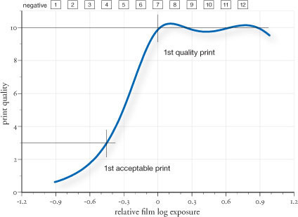
fig.1       A historic study proved that final print quality increases with film exposure.

fig.2a    Overexposing film by 1 stop increases all negative densities by similar amounts, and only requires a small paper contrast correction to print well. Print quality is not degraded. A relatively high local average gradient provides increased shadow contrast and separation.

fig.2b    Film with normal development but overexposed by 1 stop and slightly corrected print contrast. This print has more shadow detail separation than the normal print.

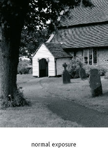
fig.3       Normal film exposure and development printed on grade-2 paper as a comparison. This print has a full tonal scale and plenty of highlight and shadow detail.

fig.4b    Film with normal development but underexposed by 1 stop and slightly corrected print contrast. This print lost shadow detail but is acceptable for standard photography.

fig.4a    Underexposing film by 1 stop decreases all negative densities by similar amounts but loses important shadow detail.

fig.5a    An overdeveloped film has dense highlights and increased shadow densities. In addition, highlight separation can suffer from shoulder roll-off, but usually an ‘acceptable’ print can be made by compensating with a soft paper grade.

fig.5b    Film with normal exposure but overdeveloped by 75% and printed on grade-0.5 paper. This print appears less sharp, because it lacks highlight and midtone contrast, but shows increased shadow detail.

fig.6       Normal film development and exposure printed on grade-2 paper as a comparison. This print has a full tonal scale and plenty of highlight and shadow detail.

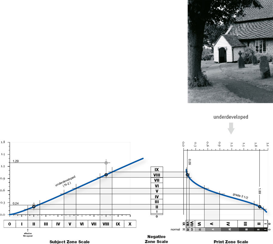
fig.7a    An underdeveloped film has weak highlight densities, but a good print can still be made by compensating with a harder paper grade.

fig.7b    Film with normal exposure but underdeveloped by 40% and printed on grade-3.5 paper. This print is almost identical to the normal print but has slightly lighter midtones.

Exposure Deviation

Fig.2b shows a print from a negative that was over-exposed by 1 stop and slightly contrast corrected during printing, as described above. Fig.2a illustrates that overexposing film by 1 stop pushes shadow and highlight densities up the characteristic curve, increasing all negative densities by similar amounts. Only a small paper contrast correction was required to make a quality print. However, the toe of the characteristic curve has lost its typical shape and has been replaced with a higher average of local shadow gradient, which indicates increased shadow contrast and separation, as is most visible in the upper half of the tree trunk. It will not be difficult to make a quality print from this overexposed negative, leaving others to wonder what your secret is to achieve this level of shadow detail.

The 1-stop underexposed print in fig.4b and its graph in fig.4a tell a different story. Shadow detail has suffered from the lack of exposure. Underexposing film by 1 stop pushes shadow and highlight densities down the characteristic curve, decreasing all negative densities by similar amounts, but rendering shadow densities too thin to retain enough detail for a quality print. Nevertheless, a slightly increased paper contrast has salvaged the print to a point acceptable for standard photography, where the untrained eye may not find objection, although a quality print can never be made from this underexposed negative.

When in doubt about exposure, I prefer to err on the side of negative overexposure for fine-art prints. There are some unwanted side effects, such as longer printing times and potentially larger grain, which is more of a concern for 35 mm users, but the final image will be of high quality. On the other hand, an under-exposed negative lacks the shadow detail required for a fine-art print, although it can still be used to make an acceptable image.

Development Deviation

Fig.5b shows a print from a negative that was exposed normally but overdeveloped by 75% to simulate an N+2 development. Fig.5a reveals that the negative highlight density increase is several times greater than the increase in shadow density. This increases the negative density range and requires a soft-grade paper to contain all textural densities. As a consequence, highlights and midtones are compressed, and shadows are expanded. The print appears less sharp, lacks highlight and midtone contrast, but shows increased shadow detail. Producing a quality print from an overdeveloped negative is difficult or impossible and requires extensive dodging and burning.

Fig.7b shows a print from a negative that was exposed normally but underdeveloped by 40% to simulate an N-2 development. In this case, a grade 3.5 paper was required to make a full-scale print from the limited negative density range and match the shadow densities of the door. Fig.7a illustrates how print highlight and shadow densities are at normal levels, but midtone densities are slightly shifted towards the highlights. The same can be seen in the print, which is almost identical to the normal print but has slightly lighter midtones. It is not difficult to make a quality print from an underdeveloped negative.

In a side-by-side comparison, the underdeveloped negative printed on hard paper has more sparkle than the overdeveloped negative printed on soft paper. However, underdevelopment results in a loss of shadow detail if not compensated with increased film exposure, as it would not be if the underdevelopment was accidental. On the other hand, the overdeveloped negative has plenty of shadow detail, but the low paper contrast appearance is just not attractive enough to consider this salvage technique for quality prints.

In conclusion, the advice from the old masters of overexposing and underdeveloping film, when in doubt, has proven to be sound even when using VC papers. The technique insures plenty of shadow detail, high local contrast and apparent sharpness.

 

Exposure Latitude

What can we get away with?

A good negative has plenty of shadow and highlight detail and prints easily on normal graded paper. We aim to create such a negative by controlling film exposure and development as closely as we can. Sufficient film exposure ensures adequate shadow density and contrast, and avoiding film overdevelopment keeps highlights from becoming too dense to print effortlessly.

Irrespective of our best efforts, exposure variability is unavoidable, due to various reasons. Shutters, apertures and lightmeters operate within tolerances, lighting conditions are not entirely stable, films don’t respond consistently at all temperatures and all levels of illumination, and no matter how hard we try, there is always some variation in film processing. Sometimes we get lucky, and the variations cancel each other out. Other times, we are not so lucky and they add up.

Considering all this, it is surprising that we get usable negatives at all. Conveniently, modern films are rather forgiving to overexposure. The ‘film exposure scale’ is the total range of exposures, within which, film is capable of rendering differences in subject brightness as identifiable density differences (fig.1). Compared to the subject brightness range (SBR) of an average outdoor scene (about 7 stops), the typical film exposure scale is huge (15 stops or more). However, the entire exposure scale is not suitable for quality photographic images. The exposure extremes in the ‘toe’ and ‘shoulder’ areas of the characteristic curve exhibit only minute density differences for significant exposure differences, providing little or no tonal differentiation or contrast.

fig.1       Film exposure latitude is defined as the range of exposures over which a photographic film yields images of acceptable quality.

Therefore, the useful exposure range, suitable for recording quality photographic images, is somewhat smaller than the total exposure range. Still, it is significantly larger than the normal subject brightness range and, consequently, offers leeway or latitude for exposure and processing errors. The limits of the film exposure latitude depend on how much image detail is required in shadows and highlights in order to consider it a quality print. This debate has already filled numerous papers and volumes of books on photographic image science. For practical photography, we can define the film exposure latitude as the range of exposures over which a photographic film yields images of acceptable quality. Most modern films have an exposure latitude of 10 stops or more after normal processing, and if you process your own films, this range can be extended substantially.

Controlling Latitude

Exposure latitude is a material characteristic influenced by development. Film exposure latitude is governed partially by the film’s material characteristics but mainly by film development. In general terms, fast films have more exposure latitude than slow films, and latitude decreases with extended development. The shorter the film development, the wider the exposure latitude (fig.1).

Zone System practitioners modify film development times (expansion and contraction) to control the useful exposure range (latitude) on a regular basis. However, they do so in an effort to match the exposure range of the film with the subject brightness range of the scene and not to provide compensation for exposure errors. It comes as no surprise that Ansel Adams (1902-1984), the father of the Zone System, never used the word ‘latitude’ in his famous three-volume series of books (The Camera, The Negative, The Print). Nevertheless, when in doubt, it is better to err on the side of underdevelopment, allowing for more exposure latitude. A ‘soft’ underdeveloped negative has better highlight separation and is, therefore, easier to print than a harsh overdeveloped negative.

fig.2       A considerable portion of the film exposure latitude is consumed by the subject brightness range. As a result, the remaining latitude depends largely upon the subject contrast.

fig.3       Strictly speaking, film has no latitude towards underexposure unless, for the sake of getting some kind of an image, we are willing to sacrifice image quality and the loss of shadow detail.

fig.4       These images illustrate the influence of under- and overexposure on image quality. All prints were made of negatives from the same roll of film, highlight densities were kept consistent through print exposure and an effort was made to keep shadow densities consistent by modifying print contrast. Prints from the overexposed negatives show no detrimental effect on image quality. Prints from the underexposed negatives show a significant loss of image quality.

A considerable portion of the film exposure latitude is consumed by the subject brightness range. As a result, the remaining latitude depends largely upon the subject contrast. The higher the subject contrast, the smaller the remaining latitude (see fig.2). The subject brightness range of a high-contrast scene, with deep shadows and sunlit highlights, is often beyond the useful exposure range of a normally processed silver-based B&W film. This leaves no latitude for exposure errors. In cases like this, normal development creates highlights too dense to print on normal paper without some darkroom manipulations or extended highlights with reduced tonal separation. However, a reduction in film development (expansion) keeps the highlights from building up too much negative density, which yields a negative that is much easier to print.

When B&W photographers depend on lab services to process their films, they usually give up latitude control through film development. At this point, the choice of film remains the only control over exposure latitude. As stated above, the faster the film, the wider the exposure latitude. Therefore, films like Delta-400, HP5, TMax-400 or Tri-X Pan are good choices, but there is an additional option.

Normally developed Ilford XP2, a dye-based B&W film, has more exposure latitude than any other film I have used. This film has a particularly extended and delicate highlight response. I never came across a subject brightness range that proved to be too much for this fine-grain film. XP2 is developed using the common Kodak C41 color negative process, and consequently, any consumer lab can develop the film. XP2 negatives print well and with ease on harder than normal contrast papers. Expose XP2 at EI 200 to get more shadow detail, and use it for normal and high-contrast subjects. However, XP2 is too ‘soft’ for low-contrast subjects, even if developed for twice the normal development time.

Kodak and Fuji also make dye-based B&W films, but they are quite different products. These films are optimized for monochrome printing on color paper in consumer labs, but they do not print as easily on variable-contrast B&W paper as Ilford XP2 does.

Latitude and Image Quality

In figures 1 and 2, we looked at the film exposure latitude as something exclusively affecting overexposure, keeping shadow exposure constant. And, ignoring a slight increase in grain size, there is no loss of visible image quality with overexposure, unless the overexposure is exorbitant, at which point enlarging times become excessively long.

Strictly speaking, film has no latitude towards underexposure (see fig.3), because film speed is defined as the minimum exposure required to create adequate shadow density. Underexposed film does not have adequate shadow density. Practically speaking, however, film has some underexposure latitude if we are willing to sacrifice image quality. For example, a loss in image quality might be tolerated where any image is better than none, as may be the case in sports, news or surveillance photography.

The images in fig.4 illustrate the influence of under- and overexposure on image quality. All prints were made of negatives from the same roll of film and, consequently, received the same development. The base print (ISO 400/27°) was made from a negative exposed according to the manufacturer’s recommendation. The other six prints were made from negatives that have been under- and overexposed by 2, 4 and 6 stops. In these prints, highlight densities were kept consistent through print exposure, and an effort was made to keep shadow densities as consistent as possible by modifying print contrast. Prints from the overexposed negatives (+2, +4 and +6 stops) show no adverse effect on image quality. Actually, the opposite is true, because shadow detail increases with overexposure in these prints. On the other hand, prints from the underexposed negatives show a significant loss of image quality (-2 stops), an unacceptable low-quality print (-4 stops), and the loss of almost all image detail (-6 stops). Obviously, film has far more latitude towards overexposure than underexposure.

The aim is to be accurate with exposure and development, knowing that there is some exposure latitude to compensate for error and variation. You can get away with underdevelopment far more easily than with overdevelopment, and you can get away with extreme overexposure better than with slight underexposure. Print quality actually improves with modest overexposure but is very sensitive to underexposure. Overdeveloped negatives will not print easily, but minute underdevelopment is easily corrected with a harder grade of paper. Film exposure latitude is what you can get away with, but when in doubt, overexpose and underdevelop.

 

Pre-Exposure

A double take on film exposure

There are occasions when subject shadows need some extra illumination, either to lessen overall contrast or to get just a hint of detail into otherwise featureless blacks. Of course, just adding some light locally, through spotlights or electronic flash, would be the best solution, but that is not always practical and sometimes impossible. Alternatively, simply increasing the exposure and reducing development may not be suitable for aesthetic reasons. This technique is always accompanied by an overall contrast reduction, adding some shadow detail, but at the cost of reduced midtone and highlight separation.

A valuable option is to precede the actual image exposure with a low-intensity pre-exposure. As the name suggests, this is a small uniform exposure, not forming an image itself, but adding some low-level density prior to the image exposure. The goal is to increase shadow density without significantly affecting midtone or highlight density and contrast. This procedure works, because the low-intensity pre-exposure has a substantial effect on the low-level shadow exposures, but is of little to no consequence to the comparatively larger midtone and highlight exposures. The outcome of pre-exposure is a modified film characteristic, with an overall lower contrast index, but uniquely, with most of the contrast reduction confined to the shadow regions. This makes the results of pre-exposure very different to modified development or simply using variable-contrast papers.

fig.1       The theoretical contribution of a Zone-II pre-exposure, in percent, halves for each increasing image Zone, until its effect becomes negligible beyond Zone V.

The optimum pre-exposure is low enough to just boost, and not overtake, the shadow exposure, but this will always add enough exposure to increase the fog level of the film. The results of pre-exposure are, consequently, very similar to usage of equipment with considerable lens and camera flare. Ironically, the photographers of the last centuries benefited from accidental pre-exposure in many of their images, as their uncoated optics were prone to lens flare, which added a low-level exposure to the entire frame. Was this the secret of the old masters?

Nevertheless, for photographers who prefer using graded papers, the pre-exposure technique offers a unique opportunity to modify the film characteristic to match their fixed-contrast papers without changing development and overall negative contrast. The same is true for roll-film users, who would rather modify the negative contrast of a single frame than to rely on the overall contrast change of a variable-contrast paper. In any case, this technique requires a camera with multiple-exposure capability.

Theory and Testing

A Zone-I pre-exposure is defined as taking a Zone-V exposure reading of a uniform subject and reducing the exposure by 4 stops. Similarly, a Zone-II pre-exposure is defined as the same exposure reading, reduced by 3 stops and so on. Fig.1 shows the theoretical contribution and overall change from a Zone-II pre-exposure to a full range image exposure. For this level of pre-exposure, those areas of the image that are placed on Zone II will receive 100% or 1 stop more light, those on Zone III will receive 50% more exposure and so on. The pre-exposure contribution, in percent, halves for each increasing image Zone, until its effect becomes negligible beyond Zone V.

fig.2       Shown below are the commercially available ExpoDisc and examples of homemade pre-exposure devices for a round filter system, which are made from a white translucent plastic. The measured exposure through the diffuser must be reduced by 2, 3 or 4 stops for Zone III, II or I pre-exposures, respectively.

To determine the actual negative response to pre-exposure, several films were tested by first applying pre-exposures of varying intensities and then photographing a Stouffer transmission tablet. All films were identically processed using the same developer, and the film characteristic curves were measured and plotted. As an example, the results for Fuji Neopan Acros 100, adding three low-intensity pre-exposures, are shown in fig.3, and they confirm the theoretical values of fig.1.

We can see from fig.3 that the pre-exposure adds significantly to the negative shadow density, while having little effect on midtone density and leaving highlight density practically untouched. However, a Zone-I, II or III pre-exposure progressively increases the negative fog level and reduces shadow contrast.

The speed point of a film is defined as having a fixed density above base and fog. Since a pre-exposure increases the negative fog level, it takes additional exposure to reach the speed-point density. Consequently, the theoretical film speed gradually decreases with pre-exposure and does not increase, as is often proposed in other photographic literature. An increase in absolute shadow density must not be confused with an increase in film speed.

Every film type has a slightly different response, depending upon the ‘toe’ shape of its film characteristic, suggesting that personal testing is required to determine the optimal pre-exposure intensity.

Making Pre-Exposures

In the chapter ‘Filters and Pre-exposure’ in his book The Negative, Ansel Adams illustrates this technique with two practical examples. His technique and that of Barry Thornton, explained in his book Elements, differ slightly in approach, although they both make their pre-exposures through a white diffuser. These diffusers are visually opaque to prevent any image forming on the film. For that reason, diffuser filters, used to soften portraits or create misty effects, are not suitable. A piece of white translucent plastic, mounted in a square filter holder, or cut into a circle and mounted in an old filter ring, makes for an ideal diffuser, see fig.2. It is an effective and economical homemade pre-exposure device. A more expensive solution is the commercially available ExpoDisc. It sandwiches a white diffuser behind a multifaceted lens, also turning into an adaptor for measuring incident light with the aid of a TTL meter, or determining the white-balance setting for digital cameras.

To ensure an accurate pre-exposure calculation, the diffuser is placed over a spotmeter, and an exposure reading is taken, using the same incident lighting conditions as will occur when the diffuser is placed over the lens used for image making. Alternatively, cameras with TTL metering may meter directly through the diffuser attached to the taking lens. In both cases, the indicated exposure is reduced by 2 - 4 stops to place the pre-exposure on the desired shadow zone. This can be done by temporarily increasing the shutter speed or reducing the aperture. After the pre-exposure is made, the diffuser is removed and the camera’s multiple-exposure device is enabled to allow for a double-exposure. Then, shutter speed or aperture is reset and the main image exposure is made on top of the pre-exposure.

In Practice

The principal use of pre-exposure is not to improve shadow detail, since a simple increase in image-forming film exposure is the best way to do that. It is apparent from fig.3, however, that a pre-exposure reduces shadow contrast and, consequently, overall negative contrast. This is the clue to its principal application. Pre-exposure can enable a high-contrast scene to print normally on fixed-grade paper, and it is a method to reduce individual negative contrast on roll film. In addition, unlike the effect of reduced development or the use of lower-contrast paper, the midtone and highlight separation of a print, made from a pre-exposed negative, is unchanged.

Fig.4a-c show the same image, made from different negatives, but all prints were made on the same fixed-grade paper, while optimizing the highlight exposure. All negatives were given the same image exposure, determined by placing the pew-end on Zone I. However, the film exposures for fig.4b and 4c were preceded by a Zone-II and III exposure, respectively. The prints have an almost unchanged highlight and midtone appearance, but the shadows gradually lighten with increasing pre-exposure, and therefore, image detail seems to progressively extend into the lower print zones.

This definitely improved the image in fig.4b (Zone-II pre-exposure) as compared to fig.4a (no pre-exposure), but in fig.4c (Zone-III pre-exposure) the effect is overdone. The negative with a Zone-III pre-exposure has a fog level high enough to veil the shadow appearance at this print exposure setting. This might not be apparent on some images, but here, with large areas of uniform dark tone, it is noticeable and undesirable.

By way of comparison, a normal or high-contrast negative without pre-exposure may also be printed on variable-contrast paper, with its contrast setting lowered to lighten shadows and making detail more visible. This is similar to reducing film development for a high-contrast scene when dealing with graded papers. Fig.6 shows another example of printing the negative without pre-exposure, but this time, at a lower paper grade. Compared to fig.4a, made from the same negative, it has lighter shadows and we can see more detail; however, the highlight and midtone separation suffers. Compared to fig.4b or 4c, it shows greater shadow separation but, unfortunately, at the same expense. See fig.7, 8 and 9 to analyze and compare the tone reproduction of the prints shown in fig.4a, 4b and 6, respectively.

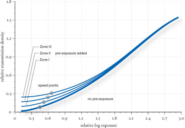
fig.3       This graph illustrates the film characteristics for Fuji Neopan Acros 100, including Zone I, II and III pre-exposures, rated at EI 50 and given normal development in D-76 1+1. The pre-exposures add significantly to the negative shadow densities, while having little effect on midtone density and highlight densities. However, pre-exposure progressively increases the negative fog level and reduces shadow contrast, which despite increased shadow densities, gradually decreases film speed.

fig.4a-c This print sequence shows the effect of increasing film pre-exposure, when printed on fixed-grade paper with the exposure optimized for the highlights. From left to right, no pre-exposure, Zone II and III pre-exposure. Note how the shadows lose their luster in the print from the Zone-III pre-exposed film. It is easy to take pre-exposure too far.

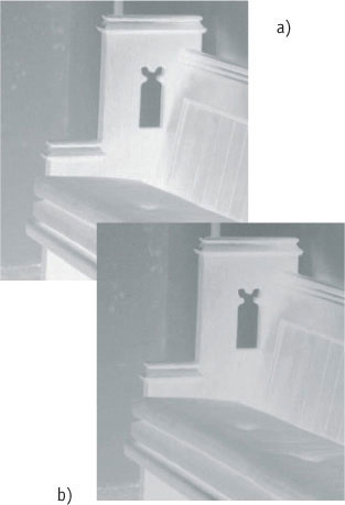
fig.5a-b One claim, often made by the proponents of pre-exposure, is that the additional exposure takes the film beyond the threshold of density development and, therefore, adds additional shadow detail. A close-up of the negative’s near-Zone-I shadow region, without (a) and with (b) pre-exposure, does not conclusively verify this claim, but the reduction of shadow contrast in (b) is obvious. Be that as it may, any additional deep-shadow detail is likely to be too dark for detection in the print anyway.

As a final alternative, one may be intrigued with printing a pre-exposed negative onto variable-contrast paper, with its contrast settings matched to the reduced negative density range. Unfortunately, this turns out to make little sense, as it does more harm than good. The reduced negative shadow contrast pushes most shadow detail onto very low print values, where it hides in the dark. A sample print of this is not featured here, but fig.10 shows the tone reproduction for verification and comparison.

In conclusion, the successful deployment of pre-exposure is wholly dependent upon the image content and is most effective when limited to fixed-grade papers. Combining film pre-exposure with variable-contrast printing is either not necessary, as fig.6 shows, or has potentially a negative effect, as fig.10 demonstrates. Since our brain is adept at spanning lighting extremes, it may not be easy to identify when pre-exposure will be beneficial. Reducing subject values to monochrome, by using a special viewing filter, will quickly improve tonal perception and exposure planning. However, only careful measurements with a spotmeter are likely to give trustworthy results.

It is also worth comparing the effect of pre-exposure with that of print flashing, whose contrary effect reduces highlight separation and maintains shadow appearance. This is explained with examples in a separate chapter, called ‘Print Flashing’.

Further Variations

In this chapter, we have concerned ourselves with ‘fogging’ exposures made prior to the actual image exposure. The term ‘fogging’ refers to an exposure level that is higher than the film exposure threshold, whereas ‘flashing’ refers to a light level below that same threshold and does not, by itself, change negative density. Jacobson and Jacobson, in the chapter ‘Increasing Film Speed’ from their book Developing, suggest further variations on the theme of pre-exposure. These include changing the timing and intensity of the ‘fogging’ exposures to alter the apparent speed and reciprocity characteristics of film. They define pre-treatment as hypersensitization and post-treatment as latensification. These treatments may be chemical or exposure-based and are not only of pictorial value, but also of practical value to those recording the extremely low-intensity objects encountered in astrophotography.

The authors suggest that light of a very low intensity is more effective at increasing an existing latent image than in overcoming the film’s threshold for a new one. This indicates that post-exposure is more potent than pre-exposure. As part of Chris’s preliminary investigation, these proposed variations were evaluated in two stages: first by evaluating the timing of the exposures and second, by evaluating the intensity of the ‘fogging’ exposure. In the first experiment, identical pre- and post-exposures were applied to an image using the same fogging intensity. The developed negatives were, for all practical purposes, identical and did not bear out the suggestion.

A second round of experimentation compared preand post-exposures using different light intensities. Jacobson and Jacobson recommend fogging the film, after the main exposure, to an extremely dim light in a darkened room, for a 30-minute duration. This is not a very practical proposition, since it is neither easy to establish or measure such a light intensity, nor is it pragmatic to expose film for 30 minutes, especially when battery-powered shutters are in use.

fig.6       An alternative to pre-exposure is to print a normal or high-contrast negative without pre-exposure on variable-contrast paper, with its contrast setting lowered to lighten shadows and making detail more visible. Here the same negative as used for fig.4a was printed, but this time, at a lower paper grade. Compared to fig.4a, it has lighter shadows and we can see more detail, but only at the expense of reduced highlight and midtone separation. Compared to fig.4b or 4c, it shows greater shadow separation but, unfortunately, at the same expense.

A final test, within the practical confines of available equipment, compared the effect of a brief high-intensity fogging-exposure (1/125 s) to a long low-intensity fogging exposure (8 s) of equal energy, but using two film types of very different reciprocity characteristics. The fogging exposures were tried both before and after the main exposure, to complete the analysis. The outcome showed some minor differences, not entirely explained by shutter tolerances and not consistent between the two films. This may be an interesting avenue for further research but is not of any particular value for image making. For further reading, we also recommend The Theory of the Photographic Process by Mees and James.

Consistency is important, and we recommended to preferably use the same aperture for the pre-exposure and the actual image exposure, since the outcome is in keeping with the theoretical sensitometry.

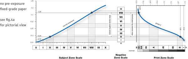
fig.7       This is the tone reproduction cycle for a normal negative, printed on normal fixed-grade paper. Note that the textural negative density range equals the textural paper log exposure range, and Zone-II shadows have typical densities of around 1.89.

fig.8       This is the tone reproduction cycle for a Zone-II pre-exposed negative, printed on the same fixed-graded paper as in fig.7. Note that the upper portion of the paper characteristic curve is not utilized. The print has an almost unchanged highlight and midtone appearance, but shadows are lighter and have less contrast. However, lighter shadow detail is easier to see.

fig.9       This is the tone reproduction cycle for a normal negative, printed on a lower paper contrast to match Zone-II shadows densities with fig.8. Compared to fig.7, it has lighter shadows and we can see more detail, but only at the expense of reduced highlight and midtone separation. Compared to fig.8, it shows greater shadow separation but, unfortunately, at the same expense.

fig.10     This is the tone reproduction cycle for a pre-exposed negative, printed on variable-contrast paper, to accurately match the reduced negative density range. However, doing so makes little sense. The reduced shadow contrast of the negative pushes most shadow detail onto very low print values, beyond human detection. The whole print will be too dark.

 

Applied Zone System

Contrast Control with development or paper grades?

Zone System basics are easy to understand, but mastery comes only with a full comprehension of its role within the complete photographic process. It is important to realize that the Zone System is not an exclusive technique but only a building block for a quality print. It does not replace other darkroom techniques but promotes them from rescue operations to fine-tuning tools. The Zone System ensures a good negative as a starting point, because it is important to have plenty of detail in shadows and highlights. Nevertheless, only additional printing techniques turn a good print into a fine print. I recommend the Zone System to control overall negative contrast and to fine-tune local image contrast during printing, as demonstrated in the following examples.

Local and Overall Contrast

Global or overall contrast is the difference in brightness between the lightest and darkest areas of a subject, negative, image or print. Local contrast refers to the brightness difference within a restricted area. Fig.1 is an image of modest overall contrast between an illuminated wall on the right and the wall in shadow, but the local contrast for each wall is rather low.

Figures 2a&b are two prints of a high overall contrast scene, made from the same negative and both printed on grade-2 paper. The subject brightness range between the sunlit window and the shaded dark wood in the foreground (overall contrast) was more than the film could handle with normal development. Nevertheless, the brightness ranges within the windows and within the interior of the room (two local contrast areas) were actually low. Fig.2a was printed with the exposure optimized for the shadows to reveal detail in the room’s interior. fig.2b was printed with optimized highlight exposure to reveal detail in the windows. Neither print is satisfactory, because either shadow or highlight detail is clipped and lost, but together they clearly reveal that the necessary negative detail is available to make a good print.

fig.1       This image has a modest overall contrast between the illuminated wall on the right and the wall in shadow, but the local contrast for each wall is rather low.

fig.2       A high-contrast scene combined with normal film development creates dense negative highlights, but a soft grade-0.5 paper is used to salvage the image (fig.2c).

fig.2c    Same negative as for figures 2a&b but printed with grade-0.5 filtration, as shown in fig.2. Highlight and shadow detail are maintained at the expense of local contrast.

fig.3       An intentional film underdevelopment extends the subject brightness range and creates negative highlight densities printable on normal paper (fig.3a).

fig.3a    New negative with reduced film development (N-2) and printed on grade-2 paper, as shown in fig.3. Highlight and shadow detail are maintained similar to the soft paper grade in fig.2c, but again, at the expense of local contrast.

fig.4       A low-contrast scene combined with normal film development creates weak negative highlights, but a hard grade-4.5 paper is used to make a good print (fig.4c).

fig.4c    Same negative as for figures 4a&b but printed with grade-4.5 filtration, as shown in fig.4. Highlight and shadow detail are maintained with increased local and overall contrast.

fig.5       An intentional film overdevelopment increases the negative density range and improves highlight densities, to print well on normal-grade paper (fig.5a).

fig.5a    New negative with extended film development (N+2) and printed on grade-2 paper, as shown in fig.5. Highlight and shadow detail are maintained similar to the hard paper grade in fig.4c.

fig.6a    The same negative as for fig.6a and printed on the same paper grade, but exposed to optimize the shadow detail. In this case, most highlight detail is lost.

fig.6b    High contrast scene, normal film development and printed on grade-2 paper. The print was exposed to optimize the highlight detail, but most shadow detail is lost.

fig.6c    Same negative as for figures 6a&b but printed with grade-0.5 filtration. Highlight and shadow detail are maintained at the expense of local contrast.

fig.6d    Same negative as for Figures 6a&b, but print received the base exposure of fig.6b, and the highlights received an additional burn-in exposure to show the same detail as fig.6a.

fig.7       New negative with reduced film development (N-2) and printed on grade-2 paper. Highlight and shadow detail are maintained similar to fig.6c, again at the expense of local contrast.

Figures 4a&b are two prints of a low-contrast scene, made from the same negative and both printed on a grade-2 paper. The overall subject brightness range between the bright wall and the shadow below the bottom stair is too low for normal film development. Fig.4a was printed with the exposure optimized for the highlight detail on the wall. Fig.4b was printed with optimized shadow exposure. Neither print is satisfactory, because they capture all negative detail available but are too soft to make for a realistic-looking print. We have a few techniques at our disposal to unlock the detail in figures 2a&b and improve the contrast in figures 4a&b.

Adjusting Print Contrast

A normal-contrast negative prints well on grade-2 paper. If the contrast is above normal, as in figures 2a&b, a softer paper grade rescues the print. This was done to produce the print in fig.2c, using a soft grade-0.5 filtration. Otherwise, it is a ‘straight print’, meaning no print manipulation such as dodging & burning was applied. The print shows all highlight and shadow detail, but at a terrible cost to local contrast. The interior of the room appears flat, gloomy and unattractive.

If the negative has a below-normal contrast, as in figures 4a&b, a harder paper grade is used to compensate for it. This was done to produce the print in fig.4c, using a hard grade-4.5 filtration. Otherwise, it is a straight print without any dodging & burning. The print has greatly benefited from increased overall and local contrast and looks far more realistic now.

Adjusting Film Development

The main purpose of the Zone System is to optimize film exposure and overall negative contrast. To create the print in fig.3a, an additional negative was prepared, placing the interior shadows on Zone III and reducing the film development to N-2 to control the highlights in the window. This captures the entire subject brightness range, and the negative printed well on grade-2 paper, maintaining highlight and shadow detail but, similarly to the print in fig.2c, at the expense of local contrast. Using paper-grade or film-development adjustments in order to harness high overall-contrast scenes with normal or low local contrast does not deliver attractive results.

To create the print in fig.5a, an additional negative was prepared, placing the shadow below the bottom stair on Zone III and increasing the film development to N+2 to raise the tonality on the white wall. This increased the negative density range to normal, and the negative printed well on grade-2 paper. Similar to the print in fig.4c, the print in fig.5a greatly benefitted from an increase in negative contrast. Using paper-grade or film-development adjustments in order to compensate for a lack in overall subject contrast works well and delivers attractive results.

Dodging & Burning

Unfortunately, dodging & burning are often considered to be nothing more than salvaging techniques for a less than perfect negative, but they are really invaluable print controls. Most of Ansel Adams’ gorgeous prints were brought to perfection through heavy manipulation with dodging & burning. This technique maintains or adds local contrast, while bringing forward the otherwise missing detail to selected shadows and highlights. In fig.6d, the advantages of the prints in figures 6a&b are combined. Using the same negative and paper contrast, this print received one overall exposure to show shadow detail as in fig.6a, and the highlights received an additional burn-in exposure through a custom mask (not shown) to reveal the same detail as in fig.6b. For comparison, the already failed attempts to control the high overall contrast of this scene through paper-grade adjustment (see fig.6c) or film-development adjustment (see fig.7) are also shown.

Contrast Control Techniques Compared

From statements made over the decades, it seems that you can only use one contrast control technique at a time. Statements such as “The Zone System eliminates the need for dodging & burning” or “Variable Contrast papers have eliminated the need for the Zone System” seem to persist in spite of evidence to the contrary. Alone, neither one of these techniques is an optimum solution, but a careful combination of them will create the best possible print.

fig.8       The evaluation of over 1,000 amateur negatives reveals the normal distribution of negative density ranges. The average amateur negative has a density range of 1.05 and, consequently, prints well on a grade-2 paper. Few negatives are outside the paper’s capability and end up with clipped highlights or shadows, but marginal negatives leave little room for creative manipulation.

fig.9       Empirical data shows that hard negatives print better on harder paper than expected, and soft negatives benefit from softer paper than expected. This is reflected through the equation of aesthetic conversion, but its application makes for softer prints than typically found in the amateur field.

As shown in figures 2 through 5, there is indeed little difference between a paper-contrast adjustment and film-development adjustment. In a straight print, both achieve very similar results in very different ways. If negative or paper contrast is adjusted appropriately, a straight print captures the entire overall contrast with either technique, and prints with matching highlights and shadows can be made. All other tones are controlled by the interaction of the individual film and paper characteristic curves (image gradation). However, negative or paper-contrast adjustments alone only work well for low contrast scenes. High-contrasts scenes usually suffer from unattractive local contrast after such treatment.

Consequently, high-contrast scenes ought to be controlled with adjustments in film development or paper contrast up to a point, but the examples in figures 6 and 7 show that high overall contrast, combined with normal or low local contrast, is best controlled with dodging & burning. Fig.6d, where this was done, is the best print of the group. Use the Zone System and film-development adjustments to control extreme contrast situation, but avoid over-reduction of normal or low local contrast. This will allow for a straight print, but it will also be a dull print.

A straight print is rarely the aim anyway, because it seldom creates a fine print. A straight print of a high-contrast scene will always suffer from lack of tonal separation due to tonal compression. This problem can be better fixed with dodging & burning. In some cases, however, it does make sense to create a fully contrast-adjusted negative first. If dodging & burning is applied to such a negative, the entire spectrum of softer and harder paper grades are available to control local contrast. This is a flexibility not available if a paper-contrast adjustment was already needed to compensate for a less than perfect negative.

From Negative Density Range to Paper Grade

Fig.8 illustrates the results of an evaluation of over 1,000 amateur negatives, which reveals the normal distribution of negative density ranges. The average amateur negative has a density range of 1.05 and, consequently, prints well on a grade-2 paper. Few negatives are outside the paper’s capability and end up with clipped highlights or shadows, but marginal negatives leave little room for creative manipulation.

In ‘Tone Reproduction’, we illustrated how the textural negative density range turns into the textural paper log exposure range when the negative is projected onto the paper. It is well known that a negative with a short density range must be printed on a positive material with a short exposure range and vice versa. Since density and exposure range are both measured in log units, we logically assumed a straight conversion. A 0.3 change in negative density simply requires a 0.3 change in paper log exposure. In ‘Measuring Paper Contrast’, we will show how textural paper exposure ranges are grouped into paper grades. Consequently, we found a straight conversion from negative density ranges to paper grades and followed it through the rest of the book. However, there is a another way of looking at this conversion.

In 1947 T. D. Sanders found an interesting empirical relationship between approximately 3,000 prints made from 170 negatives during Loyd A. Jones and H. R. Condit’s 1941 study. The analysis of the statistical print judgment from 30 independent observers revealed that for maximum print quality a surprising rule had to be followed. For soft papers, the density range of the negatives exceeded the log exposure range of the paper, while for hard papers, the negative density range was smaller than the paper exposure range. In other words, hard negatives printed better on slightly harder paper than expected, and soft negatives did benefit from slightly softer paper than expected. Fig.9 shows this empirical relationship graphically.

It should be mentioned that prints following this relationship are somewhat softer than typically found in the amateur field, but were, in the opinion of the 30 observers, of superior photographic quality. You may try both, the straight and the aesthetic negative density range conversion, to find a matching paper grade and judge for yourself.

Final Thoughts about Successful Contrast Control

From my own work, I can make the following recommendations. Use the Zone System to determine adequate shadow exposure, and adjust negative contrast through development. Watch for local and overall contrast, and do not try to cover the entire subject brightness range in high-contrast scenes. A careful practitioner visualizes important shadow, highlight and midtones of the scene and realizes that isolated highlight extremes are better burned-in at the printing stage. Dodging and burning are valuable print controls, not rescue operations. A straight print is rarely a fine print. In most cases, reserve paper-grade changes for creative image manipulation. Choosing a different grade of paper can also be used to salvage a less than perfect negative especially in low-contrast scenes, but the Zone System creates a better negative and provides more print flexibility. VC papers allow for additional creativity, adjusting local print contrast to add impact and emphasis. However, the combination of paper grades, Zone System and dodging & burning can handle subject brightness conditions none of these can handle on its own.

fig.10     It is often thought that 35mm photographers cannot benefit from the Zone System, because 35mm cameras do not have the flexibility of replaceable film backs. But, most mechanical 35mm camera bodies cost less than a medium-format film back. Here, three bodies are labeled for N-, N and N+ development. This way, exposures are ‘collected’ separately until each roll of film can be developed independently.

 

C41 Zone System

Contrast control with chromogenic monochrome films

There is a dark horse among the arsenal of currently available monochrome films. Chromogenic monochrome films were developed mainly to exploit the mainstream availability of C41 color processing and make monochrome imaging available to all photographers, but some of these films also produce excellent images on conventional B&W paper and also offer several other important advantages.

Since reliable C41 development is widely available throughout the world, it gives the travelling photographer the assurance of passing developed film through airport X-ray machines without the risk of ruining exposed emulsions. Chromogenic B&W films provide an extremely wide latitude towards overexposure and have a negative density characteristic that gently rolls off extreme highlights. This makes these films ideal for high-contrast situations. A chromogenic image is formed by dyes rather than metallic silver, which offers a softer grain and produces images with creamy highlights. The dyes are the reason why chromogenic films are much easier to scan than silver-based films, even at high resolutions. However, many photographers shun chromogenic B&W films for the apparent lack of contrast control during standard C41 processing and archival concerns.

This chapter addresses both concerns by exploring the capability of customized C41 development to accommodate the scene contrast, just as one would with the traditional Zone System, and by clarifying the archival properties of chromogenic materials.

fig.1       Ilford XP2 is capable of very beautiful effects especially in high-contrast conditions, in this case staring into a glaring misty sunrise. Mamiya 7, 43mm f/16, printed on Agfa Multicontrast Classic with filter 4 for the foreground and filter 0 for the sky.

My favorite chromogenic B&W film is Ilford’s XP2 Super, which I mainly use for landscape photography, especially when travelling light with my Mamiya 7. Since I do my own C41 film development using a standard C41 development kit and a Jobo CPE processor, I’m able to control chromogenic negative contrast very similarly to B&W negative contrast.

Faded Memories

Since color film technology is not considered elsewhere in this book, it is prudent to address the thorny subject of longevity first. All statements about longevity are predictions, mostly based on the outcome of accelerated fade tests under extreme environmental conditions. The acceptance criteria, as well as the test conditions, vary. For instance, claims about the lifetime of inkjet prints often refer to the point where the print has an ‘unacceptable’ appearance. That gives a wide scope for interpretation. However, with negatives, the degradation is easier to define and counteract. Unlike color prints, fading can be measured objectively with a transmission densitometer. Indeed, a common industry standard is to measure the storage time required to reduce a negative density of 1.0 by 0.1. This fading is approximately proportional to the negative density range, so in this case, the negative would require printing with an extra 1/2-grade contrast setting to recover the loss of negative density.

Chromogenic B&W films use color film technology based on three separate layers made from cyan, yellow and magenta dyes. Each dye layer has a different fading speed, cyan fading first and magenta being most stable. Fortunately, cyan has little effect with monochrome printing, so the significant image forming dyes are yellow and magenta. Manufacturers’ predictions estimate that the yellow and magenta dyes fade respectively over a range of 20-50 years and 50-100 years, by the amount described above, under typical ambient conditions. These predictions are made from accelerated tests, which are run at high temperatures, and as such, are likely to be pessimistic, since high temperatures also simulate other degradation mechanisms. The common dark storage condition for negatives, within paper or plastic sleeves, will contribute to a longer life.

Fortunately, because the negative is not the final image, a proportional density loss can be remedied by printing an old negative with a higher paper contrast to recover the tonal range. Over the same span of time, our paper supplies will change, probably forcing the printer to reprint an old negative from scratch anyway. In the case of negative scanning, the image adjustment controls in the scanning software will correct the defect. In fact, some manufacturers indicate that the useful life of a chromogenic B&W negative may well exceed that of the acetate base, which is of course used with silver-based roll films too.

To be realistic, many of us are not going to be around long enough to find out if these predictions are wrong. In all probability, I am less likely to have a problem with a treasured negative taken today on chromogenic film in my retirement darkroom than suffer the effects of poorly fixed or washed silver images. In today’s digital climate, more concern should be levied over the choice, availability and improvement of monochrome films, developers and papers over the next 10 years. This does not mean that we should not do whatever we can to protect our negatives against premature deterioration. As you would with silver-based negatives and prints, store chromogenic negatives in acid-free sleeves, at or below 20°C and between 30-50% relative humidity, and avoid unnecessary exposure to light.

Film Choice

This chapter investigates Ilford’s XP2 Super, which is similar to Fuji’s Neopan 400CN. Kodak’s T400CN was also evaluated in combination with variable contrast paper, but, in common with a number of users, the negatives did not print as predicted‚ from the measured baseboard intensity and contrast. The prints were about 1.5 grades softer than expected and about 1 stop underexposed. I concluded that the orange base and brown image reduced the amount of blue ‘hard’ light passing through the negative, altering the print contrast and exposure setting. Judging from the advertising campaign that Kodak uses, and the appearance of the negatives, I assume that T400CN is ideally suited for accurate color control with color print processing methods.

C41 Processing

At the time of writing, my local lab charges the same to develop a roll of C41 as it costs me to buy it. Push or pull development costs more. If several films are developed at once, home processing can be more convenient and cost effective, at about 1/4 of the price. The main consideration with home processing C41 films is to find a reliable method to keep the chemicals and developing tank at 38°C, and agitate evenly. The standard processing steps are:

fig.2       This table provides C41 processing times for alternative temperatures.

fig.3       To maintain consistent results, some processing-time adjustments are required when developing additional films.

1.   preheat

2.   develop

3.   stop bath or rinse

4.   bleach fix and wash

They are followed by an optional stabilization. All steps require continuous or frequent agitation. The two choices with C41 chemistry are to replenish or to replace. Small volume (300 ml) ‘press packs’ are commonly available and can process six films with ease, depending on the level of developer oxidation. Films are best developed in pairs, each subsequent pair requiring an adjustment in processing time, to allow for the reduction in chemical activity. Even with non-replenishment chemistry, developer and bleach-fix solutions are reused several times, with an appropriate extension of processing times. Most instructions recommend 5% additional development for each subsequent film, up to a given film limit.

fig.4       These are the characteristic curves for Ilford XP2 developed in a Jobo CPE-2 processor at 38°C in fresh chemistry.

Replenishment systems use a larger working volume, and use a dedicated replenisher to maintain developer and bleach fix activity. This approach is economical with high throughput, and is a way of keeping constant developing times and conditions. The replenisher approach may be more appropriate for film processors that do not over-agitate during the development cycle.

With non-replenishment chemistry, films should be processed in quick succession, otherwise the chemical activity of the working solution rapidly reduces. After developing two films, I developed another a few days later. The working solutions had been stored in their bottles with a squirt of protective spray. Even so, the image on the third film was barely visible. After some enquiry, I realized that the rotary form of agitation that takes place inside the Jobo tank introduces oxygen into the developer solution. With time, this dissolved oxygen oxidizes the active ingredients. In addition, the excellent volume efficiency of horizontal rotation (only 300 ml for two films) is another reason for ‘perceived’ developer droop, in the same way as film processing in highly dilute developers.

Hence, for maximum capacity and consistency, my advice is to use 100 ml at a time, creating 300 ml of working solution at the customary 1+2 dilution. Develop two films at a time, up to a maximum of four films, and then discard within 48 hours.

An ideal film home-processor, for use with replenishment chemistry, would have a large volume of developer solution, a vertical axis of rotation and complete full-time film immersion. This would stir in less oxygen, and so, prolong developer life.

Agitation

The processing times for C41 are relatively short. But, with monochrome film processing in an inversion tank, anything under 4 minutes is normally not recommended. With C41 development, careful agitation is required to avoid streaking. The normal inversion and twist inversion technique, that serves so well with conventional monochrome films, can give problems with C41. With just 300 ml of chemistry in a hand tank, excessive frothing of the developer from repeated inversions can cause processing marks along the upper film edge. As the volume of the active chemistry reduces with each use, potential for partial film immersion increases. In addition, the repeated removal of the tank from its water bath cools the tank quickly. Fortunately, the Jobo unit controls both temperature and agitation. The spiral tank is held on its side within the water bath and rotated back and forth, without causing developer frothing. This not only keeps ‘fresh’ developer over the surface of the film, but also enables 300 ml of chemicals to process two 120 or 135 films at a time. The original Jobo film tank (4312) does not empty particularly neatly or quickly, whereas in comparison, the latest film tank (1520) and spirals empty and fill well. In addition, the new reels have less friction enabling film to be pushed onto the reel in a matter of seconds, without endless shuffling.

fig.5       Ilford XP2 effective film speed or exposure index (EI) versus development time

Material Testing

As in earlier chapters on film development, a test target, in this case a 4x5 inch Stouffer step tablet, was photographed repeatedly onto several films.

A standard ‘press kit’ was used, 100 ml of which was diluted to make 300 ml of working solution. Since the working solution was used for several tests, each development time was referenced back to the C41 standard for that number of processed films. In this case, two half rolls were developed at a time, so the normal 5% development extension per film was applied. On my old Jobo CPE-2, the high-speed agitation setting was selected and the water bath adjusted to 39.5°C. At this temperature, the developer, at completion, was exactly 38°C. Fig.2 shows alternative processing times for different operating temperatures, and fig.3 shows the standard corrections for chemistry reuse.

fig.6       Ilford XP2 is able to compensate for different subject brightness ranges by altering the development time, just as in the traditional Zone System.

For this test, the step tablet was backlit and photographed with a 100mm lens mounted on a Fuji GX680 loaded with XP2 Super. The magnification of the image was such that the bellows compensation was exactly 1 stop. At this magnification, each density step was wide enough to be directly measured with a transmission densitometer. Camera aperture and shutter-speed accuracy had previously been verified and proved to be excellent.

Before taking any density measurements, a 13x print was made from each test film, using filter 5 to accentuate film grain. Unlike conventional films, XP2 or T400CN film grain does not appear in the highlights, but in the shadows. This is explained in the Ilford darkroom manual as a result of overlapping dye clouds, which prevent small holes printing as dark grains. There is, however, grain in the shadows, but the effect is small. The test prints were shuffled, and with some difficulty, ranked in grain size. The conclusion is that with small to medium enlargements, (10x), the grain easily outperforms a silver-halide emulsion of the same speed.

Density readings were taken from each test negative, using a Heiland densitometer. The results are plotted in fig.4. Each individual development time and temperature was recorded, so that the development times could be normalized in each case for fresh chemicals at 38°C. A note of caution: as with other processing tests, it is not always possible to reproduce exactly the same conditions in your own darkroom. This is especially true with the more critical C41 processing variables. Hence, the results in fig.4, 5 and 6 are based on my own darkroom conditions and should be viewed as an indicator.

The curves in fig.4 look conventional enough, with varying slope and foot speed. We can see that the film responds well to different levels of development and resembles standard silver-halide film curves. The 4-minute line really does tail off at high densities, giving extreme development compensation. This compensation, rather like the effect of using Pyro developer and two-bath formulae with conventional film, prevents highlights from blocking up. Many users can testify that this ability to roll off the highlights has salvaged many a high-contrast scene. Such a scene can be still be printed with good midtone separation and subtle detail in the highlights, something that is difficult to do with a silver-halide emulsion and reduced development.

Film Speed

The standard development time of 3:25 minutes produces a low-contrast negative with a speed loss of about 1 2/3 stops from the published ISO 400/27° figure, based on our standard speed point at Zone I·5 with a negative transmission density of 0.17 above base+fog. One point to note is that the effective film speed, based upon a Zone I·5 shadow reading, can vary significantly with the development time. This is shown more clearly in fig.5, where the exposure index is plotted for different development times.

Fig.4 can also be interpreted to give the expansion and contraction (N) for different development times as is shown in fig.6. However, due to the low-contrast characteristics of XP2, we cannot base our Zone System calculations on the typical 1.20 density increase (0.17 to 1.37) over 7 zones (I·5 to VIII·5), because such a density increase is not obtainable through normal development times. Instead, we have to base the XP2 Zone System on a 0.83 density increase (0.17 to 1.00) over 5 zones (I·5 to VI·5) for N-2. The average gradient is about the same for both (0.57 versus 0.55), but the lower textural density range explains why XP2 negatives are typically printed on grade-4 paper. This method has proven to work well with my papers and filters.

The unique smooth tones of Ilford’s XP2 Super and its Fuji and Kodak cousins, with their ability to cope with extremely wide subject brightness ranges, make these films worthy of merit, especially for landscapes and other high-contrast scenes. With fine grain, sensible longevity and the ability of push and pull processing, as well as the convenience of lab processing, this film has ousted most other high ISO 400/27° films from my refrigerator.