
Mining Techniques for Body Sensor Network Data Repository
Vitali Loseu1, Jian Wu2 and Roozbeh Jafari2, 1MPI Lab, Samsung Research America, 2University of Texas at Dallas, Richardson, Texas, USA
Body sensor networks (BSNs) form an important class of devices where lightweight embedded processors and communication systems are tightly coupled with the human body. BSNs can provide researchers, care providers, and clinicians access to tremendously valuable information extracted from data that are collected in users’ natural environments. With this information, one can monitor the progression of a disease, identify its early onset, or simply assess a user’s wellness. One major obstacle to wide BSN deployment is maintaining and managing an enormous amount of sensing data. To address this issue, this chapter reviews existing mining techniques and describes a data-mining approach inspired by techniques in the areas of text and natural language processing. The approach is based on representing sensor readings with a sequence of characters called motion transcripts. Transcripts reduce complexity of the data significantly while maintaining morphological and structural properties of the physiological signals. To further take advantage of the signal’s structure, the data-mining technique focuses on the characteristic transitions in the signals. These transitions are efficiently captured using the concept of n-grams. To facilitate a lightweight and fast mining approach, the overwhelmingly large number of n-grams is reduced via information gain (IG)-based feature selection. The effectiveness of the proposed approach is evaluated in terms of the speed of mining while maintaining an acceptable accuracy in terms of the F-score combining both precision and recall.
Keywords
Body sensor networks; string templates; n-grams; Patricia tree; data mining
1 Introduction
Body sensor network (BSN) research is maturing and increasingly moving from preliminary sensor, node, and network evaluation to investigation of more partial applications ranging from fall and posture detection [1,2], telemedicine, rehabilitation, and sports training [3,4]. These systems are composed of lightweight wearable sensors that capture different modalities of data from the human body. This data may include inertial measurements, electrocardiogram (ECG) readings, electromyogram (EMG) readings of the muscle activities, skin conductance level, blood pressure, and several other modalities. The diversity of applications means that the data collection setup has to be uniquely tailored for each application and the type of sensor nodes. This step can either be performed manually or considered to be a parametric optimization problem subject to the application constraints. Manual sensor selection and placement is usually based on prior knowledge of sensor efficiency in detecting a given movement or physiological phenomenon, or it is based on prior knowledge of a particular sensor-placement combination for avoiding a given type of artifact.
For example, positioning a peripheral oxygen saturation sensor on the ear is effective in reducing motion artifacts [5]. Because the ear is located close to the human vestibular system, it is exposed to limited random movements. Similarly, movements related to food intake (e.g., eating) are likely to be better observed with sensors on lower and upper arms [6]. Sensor placement and selection can also be done automatically. While this approach is more general, in a sense it can adapt to the changing application conditions, but it also requires additional resources. This can mean redundant sensor placement, increased sensory and processing load, or even increased communication load [7]. The automated optimization criteria for sensor placement can generally be classified into short-term and long-term strategies, where the former means optimization of the system for the quality of recognition, and the latter corresponds to increasing the sensor network lifetime. The short-term strategy approach can be demonstrated by maximizing the probability of detecting a target [8] or improving hazard detection by drivers on the road [9]. An example of the long-term strategy can be demonstrated by the approach that tries to optimize the network lifetime while meeting minimum sensing constraints [10]. All of the above automatic sensor management approaches only determine the initial sensor placement. They do not address imprecision of sensor placement or sensor displacement during the experiments.
Sensors of different types are often deployed by researchers, and often the experiments are highly controlled, i.e., the conditions of sensors are carefully monitored. If the sensors are to be used in natural settings, it is often challenging to ensure ideal laboratory settings, control, and monitoring would be available. This is especially true for the BSNs because it is often difficult to ensure sensor placements remain intact after the original deployment. This problem is often addressed by continuous feedback and calibration using additional sensor modalities. For example, sensor fusion of two dual-axis accelerometers and three dual-axis gyros is performed to properly estimate roll, pitch, and yaw of movement despite possible orientation changes and sensor drift [11]. A similar sensor fusion algorithm is designed for a body-worn sensor network that consists of a tri-axis accelerometer, tri-axis magnetometer, and a tri-axis gyroscope [12]. Direction cosine matrix (DCM) in the case of inertial sensors and Kalman filters are often popular choices for calibration and error correction due to the ability to both estimate the desired value and the noise in the system. Both of the above examples rely on the wearable sensor for both estimation and correction; however, that is not always desirable because the setup becomes less seamless and clunky to wear. Additionally, while a Kalman filter or a DCM-based approach are able to track the orientation change of the sensor nodes, the performance of these algorithms degrades drastically if the displacement affects the nature of the biomechanical observations.
For example, if a sensor node is to get displaced from just above the elbow to just below the elbow, the biomechanical model of the observed movement completely changes and can no longer be described by the previous estimations. This problem can be addressed via utilizing a non-wearable infrastructure. An example of such an approach can be found in an application for indoor map building, where inertial sensors are fused with environment-referenced sensors, such as ultrasonic, optical, magnetic, or RF sensors [13]. The approach works very well due to the availability of a great variety of information. It also moves some of the power consumption away from the wearable device and to a static infrastructure, where the power consumption is not as much of an issue. However, the static infrastructure is also a significant limiting factor in terms of the practical deployment and utilization, and adds costs. Context-aware data fusion is another way of tackling the original problem. Instead of directly using additional sensor modalities as input, a context-aware data fusion relies on establishing a context of a particular action to extract additional information ([14,15]).
BSN platforms are desirable because they provide a relatively inexpensive way to collect realistic and, more importantly, quantitative data about the subjects in their natural environment. Furthermore, sensor nodes can be inserted into common wearable items such as belt buckles, shoes, or pendants, which promotes the adoption by end-users. Ease-of-use in BSN nodes allows them to be quickly deployed, and data collected and processed. A problem that has not received sufficient research attention is storing and tracking the collected data. The data collected from these wearable systems are especially valuable for medical applications. The ability to search and compare BSN observations can potentially shed light on diseases such as Parkinson’s disease [16]. Parkinson’s disease is a neurological disorder, but many of its symptoms, such as slow automatic movements (e.g., blinking), inability to finish some movements, impaired balance while walking, muscle rigidity, and tremor, severely affect human movements and can be observed with the help of wearable inertial sensors [17]. Wearable nodes can enable monitoring and detection of the onset of a disease. Based on the above properties of BSNs, we envision that in the near future, large repositories of BSN data will be available. The information in such repositories can be utilized to address the problems associated with data collection, including error reduction and variations due to the subject’s unique movement execution. This can be achieved by extracting and comparing structural properties of the data. Comparison of the signals relies on the idea that similar movements have inherently similar structure, while not being exactly the same. This idea is important, because it suggests that while observations may not match in their entirety, due to the data collection artifacts and variations in individual subject performance, they still have a distinguishable structural similarity.
The real challenge with this type of approach comes with implementing all the logic on the sensor nodes to avoid a heavy communication energy cost. BSN sensor nodes are highly constrained in terms of memory, processing power, and battery lifetime. This means that not all collected data can be stored on the wearable device, communicated wirelessly for an indefinite amount of time, or processed with complicated and possibly slow computational approaches on the device itself. At the same time, the wearable devices have a potential to produce very large data sets over time. This suggests that the data representation approach needs to significantly reduce the complexity of the data, while maintaining the characteristic properties of the signal, which in our case is the signal structure. This task is further complicated by the possibility of errors in the signal and inter-subject variability in movement performance. This problem can be solved by applying limited processing that exclusively focuses on identifying unique (in terms of a given application) structural blocks and transitions between them. In the context of the activity recognition application, this approach can be further simplified to detecting transitions in the signal that uniquely characterize each movement. For this step to be successful, it is essential for the system to extract the properties of the signal capable of capturing such characteristic transitions. While in other system components (such as communication), redundancy may be acceptable and even desirable, the resource and time constraints of the BSNs demand that the considered set of signal properties be minimal. With these requirements in mind, the chapter reviews existing mining techniques and presents a novel data-mining model for large BSN data repositories based on a pilot application on human movement monitoring.
2 Machine Learning Approaches to Data Mining
The goal of data mining is identifying relevant objects. The relevance of an object may be defined by some features or parameters and its similarity to other objects. This task is trivial in a well-structured and indexed database. However, when the data is not trivially structured, defining features and measures of similarity are not obvious. Possible techniques addressing this issue can be generally partitioned into two phases. Information retrieval is the first phase, where important information for a given application is extracted from possibly noisy data. Object summarization is the second phase, where features of interest are defined in the context of relevant information extracted during the first phase. The first phase combines information theory with the properties of the specific object type. The second phase tries to identify the best way to store and parse the metadata extracted during the first phase to efficiently mine the data and identify relevant objects. Before looking into the details of BSN data mining, it is important to look into a set of basic machine learning techniques that are often used for data mining.
2.1 Mining Techniques
The most simple classification rule based on a set of instances is called 1R or 1-Rule. In this approach, the system selects one attribute of the collected sensor readings and makes a classification decision based on it. While this a very simple approach, it tends to work reasonably well for some applications [18]. The rule selection can be described as follows: For each possible attribute, the system can count how often each value of that attribute appears in any given class and make an attribute-class assignment based on the value appearing most often. It can calculate the error of all of the attributes based on the cross validation set and select the attribute with the least error. This algorithm faces two major issues: First, it may not be able to account for the values that are missing in the training set. Second, when an attribute has a large range of values, it is prone to over-fitting (or may detect trends specific to the training data that are not desired for detection and mining).
Statistical modeling is a potential solution to the problem. Instead of selecting only one attribute, the system can select all of the attributes, assuming that they are independent. Such an approach is known as Naive Bayes and can perform well when the assumptions hold [19]. The approach has two major problems. First, it assumes that each of the attributes is independent, which is likely not the case for many real problems. This problem has been extensively studied in [20,21], where the authors propose a semi-Bayes approach to modeling the actual data dependencies, correct data bias and manage attribute weights. The second problem is the assumption that the attributes have normal distribution, which may not hold in many practical applications.
Another way to address the issue of different attributes having diverse ranges is based on divide-and-conquer. Typically, this suggests creation of a tree-like structure, where each node corresponds to a specific attribute [22]. This way an attribute does not correspond to a whole level of the tree, meaning that at the same level different branches may use different attributes. This approach works in a top-down manner, where, at each level of the tree, it seeks the best attribute to split the remaining data. The difficulty of this approach lies in selecting proper attributes at levels in the tree. It often uses feature selection algorithms such as information gain [23], mutual information [24], and utility-based solutions such as Bayesian information criterion (BIC) [25]. Shortcomings of these approaches are defined by their respective assumptions. For example, information gain tends to work very well when attributes have very few possible values, suitable for binary attributes [26]. Information-gain performance decreases as the number of possible values increases due to the nature of the entropy calculations.
Previously described approaches work best with nominal attributes; however, the idea can be extended to the numerical attributes as well. The most simple and relatively effective approach is known as linear regression, where the idea is to represent class values as linear combinations of the attributes and their respective weights [27]. The idea is to calculate proper weights during the training process and apply the classifiers on the validation data. While this approach often works very well, there is a serious drawback: it assumes that the data can be modeled in a linear fashion, which may not be a valid assumption. This problem can be addressed with the help of logistic regression and then evaluated with log-likelihood maximization [28]. A major problem with this approach is probabilities not adding up to 1 when the logistic regression is applied to multiple classes.
In instance-based learning, the training trials themselves are used to evaluate unknown samples. It is done with the help of a distance function defined for the data of interest. For classification purposes, the system measures the distance from an unknown trial to the training sample and selects the one with the shortest distance. A simple example of this learning time is the 1-nearest-neighbor (1-NN) approach. However, this approach considers each attribute equally just like Naive Bayes. Additionally, a specific classification can be heavily affected by the outliers that do not represent the class well. These problems can be partially addressed by a k-NN approach, where instead of finding the nearest sample in the training data, the system looks for a consensus among k nearest neighbors [29]. However, k-NN approaches are very slow.
Clustering algorithms are applied when there is no predetermined class to be detected, but rather the observed instances are split into natural groups. During the clustering step, the instances are combined together, based on strong resemblance, to form groups that can act as classes during the detection process. There are many approaches for clustering implementation, but they mainly focus on bringing the similar instances together, while separating the dissimilar instances. One of the most commonly used clustering approaches is known as k-means [30]. It takes the training instances and the number of desirable clusters as an input and groups instances together based on their proximity. In the context of the Euclidean distance, the k-means approach iteratively minimizes the total squared distance from each instance to the cluster centers. It generally has two weaknesses. First, the best number of clusters is not always obvious, while a bad choice can result in improper grouping. Second, the iterative approach heavily depends on the initial selection of the cluster centers. Different random selections can result in significantly different clustering.
2.2 Structural Recognition in BSN
In the context of BSN data, the idea of structural data representation and recognition is explored in [31]. This approach has a major weakness. The comparison evaluation is based on the value of Levenstein distance (or edits distance) [32]. Edit distance calculation assigns the same weight to deletion, insertion, and substitution operations. It is not a problem when the compared strings have similar size. However, BSNs can observe the same movement at different speeds, which may mean that the speed of movement execution can dominate the edit distance value. It is possible to manually manage the weights of each one of the three edit distance operations; however, that would generate a heuristic approach [33]. Another way to deal with this issue is to normalize the length of each primitive in motion transcripts [34]. While this approach might work in some specific applications, in general it is very hard to predict how to scale parts of movements depending on the overall execution speed. A possible solution to this problem is to identify significant transitions in the motion transcripts and base the comparison on variations in these transitions. In the field of speech processing, a similar function is often performed by n-gram features. N-grams are substrings of length N. They were first introduced by Shannon [35] as a means of analyzing vulnerability of ciphers but since have been extensively used in the field of speech and text recognition.
N-grams [36] proved to be useful for structural parameter extraction when used for spoken language recognition [37]. N-grams can be used to capture phoneme, in the case of spoken language, and grammatical constructs, in the case of written language, to identify bodies of speech or text. Similarly, n-grams can be used to analyze text summaries [38] or translation quality [36] with respect to co-occurrence statistics. While good at recognizing major structural differences, n-grams can also be used in the case of fine grain spelling error correction [39]. In addition to maintaining structural information of the considered string, n-grams can significantly reduce the amount of information that needs to be stored and verified. Instead of storing a large body of text, the system can identify important transitions and improve both the memory usage and the execution speed of the search. These important n-grams can be better organized with a suffix tree [40], which would increase the speed of identifying language constructs [41]. In fact, suffix trees are often used to index large amounts of data in the natural language processing and other fields. For example, in the field of molecular biology, DNA sequences can be indexed with the help of suffix trees [42]. In [43] the authors discuss an efficient query algorithm on a large compressed body of text using suffix trees. The general effectiveness of the suffix trees is discussed in the work trying to identify local patterns in an event sequence database [44].
At first glance, the above examples have little in common with data collected from BSNs. Suffix tree approaches normally index a uni-dimensional data set, while BSNs normally have a set of multiple sensors with multiple dimensions of sensing. This problem can be resolved by combining all data readings and representing them with uni-dimensional primitives [31]. While this simple approach seems to resolve the issue, it fails to recognize that each one of the sensing dimensions (or individual orthogonal sensing axis of sensors such as accelerometer) can observe variations such as changing speed and amplitude of the signal. In a text data set, the variations are one dimensional, just like the data itself; this is not the case in multidimensional sensor readings of BSNs. Furthermore, it is not clear how variations occurring in multiple sensing dimensions should be handled in the context of a one-dimensional primitive. It is possible that different combinations of signal variations may hinder the structural consistency of the combined primitive representation. Classical mining techniques are not well suited for BSN data due to their inability to capture structural and relational properties of the signals and not providing a compressed data representation. Therefore, novel data-mining methodologies are required to address these shortcomings.
3 Mining BSN Data
3.1 BSN System
The BSN system in this chapter consists of a set of wearable nodes placed on the human body to collect inertial activities from human movements and a computer that maintains the BSN repository and facilitates data organization and mining. The wearable nodes are connected to the computer via wireless radios. The system overview is shown in Figure 1 and the details on the operation of the system are described in the following sections and summarized in section 7.

3.2 Wearable Sensor Hardware
Each wearable sensor has a tri-axial accelerometer (providing x-, y-, and z-axis of acceleration) and a bi-axial gyroscope (providing x and y axis of angular velocity) that is sampled at 50 Hz. This sampling frequency is high enough to provide acceptable resolution of the movements, and has been previously suggested by several investigations on physical movement monitoring applications [45,46]. Furthermore, it satisfies the Nyquist criterion [47]. After collecting the data, each node sends its readings to the base-station, which forwards all of the received data to the PC via a USB connection for further processing.
3.3 Pilot Application
To illustrate data mining in a large BSN repository, the proposed approach is applied to a classification problem, where the classification is performed by mining a database of inertial sensor data. Furthermore, as the mining approach is designed for a large data set, the aim is to make it as fast as possible. The database in this case consists of data of ten movements from three subjects. The details of the experimental movements can be found in Table 1. Every subject repeated each movement ten times. Each subject was asked to wear nine sensor nodes positioned on both ankles, both thighs, both wrists and upper arms, and one on the belt (as shown in Figure 2).
Table 1
| No. | Description |
| 1 | Stand to Sit |
| 2 | Sit to Stand |
| 3 | Stand to Sit to Stand |
| 4 | Kneeling, right leg first |
| 5 | Turn counter clockwise 90 degrees |
| 6 | Look back clockwise |
| 7 | Move forward (1 step) |
| 8 | Move to the left (1 step) |
| 9 | Move to the right (1 step) |
| 10 | Jumping |

3.4 Desirable Solution Properties
A data-mining technique for the BSN data repositories should take raw sensor readings as an input and perform a computationally efficient search in the repository to identify signals similar to the input. Due to a potentially large size of the repository, the approach needs to be fast yet reliable. Sensor readings can be viewed as observations made by the system. Upon receiving an observation as the input, the search approach should be able to identify a movement class to which the observation belongs, so that it can be stored in the appropriate place in the repository. It should be able to compare signals of two movements and find possible similarities. Furthermore, it should be able to identify similar portions of the signals, which can be useful to identify abnormality in movements. Finally, it needs to identify movements that contain certain instances of the signal (e.g., identify all movements where the torso moves forward).
4 Data Representation
A physical movement can normally be represented as a sequence of shorter motions. Capturing the structure of movement involves capturing these shorter motions and timing relationships between them. This can be done by identifying motion primitives. Following the idea introduced in [21] a clustering technique is used for primitive generation. Features are extracted from the signal and clustered. The clustering outcome is dependent on the perspective that the features can provide. This adds flexibility to the data mining because different feature sets can characterize the signal from different perspectives.
4.1 Primitive Construction
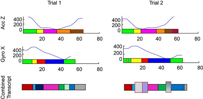
Before applying a clustering technique, it is necessary to decide what data set the clustering is applied to. One way to handle this issue is to combine all axes of sensory data to define primitives. This approach is not most suitable because, when the multidimensional data is merged into a uni-dimensional primitive, combining variations of each of the sensing axes could modify the structure of the combined primitives. An example of such an alternation can be a slight delay of the movement. This alternation does not modify the structure of the individual sensory axis signals, but, since alternations of all of the axes are independent of each other, aligning them with respect to time can significantly change the structure of the combined primitives. Figure 3 demonstrates two trials of the same movement where a slight variation in one of the axes, which does not alter the signal structure for that axis, introduces changes to final primitives. While the signals in the second trial have the same structure as the signals in the first trial, as demonstrated by the individual transcripts, their timing is inconsistent with the signals in the first trial. The bottom part of the figure demonstrates the combined transcript generated from two individual transcripts. Large vertical blocks correspond to the parts of the combined transcript of the second trial that do not have a corresponding counterpart in the first trial. This suggests, if the primitive transitions are not aligned in the original signals, the time aligned combination of these signals may not be consistent between both trials. Noise in the inertial data will introduce yet another source of error.
To avoid the issue with alignment, the reading of each sensing axis can be performed separately. Primitives are created for each one of the axes and each sensing axis is treated as a separate classifier. This approach has an additional benefit of increasing the flexibility of the system. The system does not require all of the sensing axis used in one experiment to be present in other experiments, which means that it does not dictate a particular hardware configuration.
4.1.1 Data Clustering
Clustering is a very effective method of grouping similar data points and distinguishing between different data points. When trying to cluster BSN data, a clustering approach is normally applied to feature vectors extracted from the original signals. There are a variety of features that can be extracted from inertial data. Different approaches rely on first and second derivatives, signal mean, amplitude, variance, standard deviation, peak detection, morphological features, and more. Ideally, a small and simple feature set should be identified that would produce good results. The resultant clusters should be able to identify enough transitions in the signal so that each movement of interest would be characterized with a unique subset of such transitions. A primitive generation experiment concluded that first and second derivatives are sufficient to describe the structure of this data set. To minimize the effect of the inter-subject differences in features, the system normalizes features with respect to each subject using a standard score (or z-score) [48]. In general, the proposed approach is independent of the feature selection and only requires that selected features would represent the structure of the input signal.
There is a wide array of clustering techniques that includes hierarchical, partitional, conceptual, and density-based approaches. For BSN data mining, two clustering approaches were considered. The first approach was k-Means clustering [49]. k-Means is a hierarchical approach that attempts to partition the data in a way that every point is assigned to a cluster with the closest mean, or cluster center. The second approach was expectation maximization in Gaussian mixture models (GMM) [50]. Both approaches try to identify the centers of natural clusters of the data instead of artificially selecting points in the training set as cluster centers. GMM clustering computes the probability that any given point is assigned to every individual cluster and makes an assignment that maximizes its likelihood of such assignment. Both clustering approaches are computationally simple and identify cluster centers of the data set without any prior knowledge of the data. Both approaches start with random cluster centers and re-evaluate them after each round of assignment. Once the cluster centers stay constant within a predefined threshold, both algorithms assume to have converged to the natural cluster centers of the data and return the result.
A parameter to determine during unsupervised clustering is the number of clusters k that produces the best results. To find the best solution, k was varied from 2 to the length of the shortest observation in the training set, while evaluating parameters of both k-Means and GMM. In the case of k-Means, the decision was made based on cluster silhouette [51]. Silhouette is calculated based on the tightness of each cluster and its separation from other clusters. For every point i, the silhouette is defined as
(1)
where a(i) is the average distance of point i to all other points in its cluster, bj(i) is the average distance of point i to all the points in cluster j, and b(i)=min(bj(i)), ∀j.
Silhouette s(i) describes how well the point i is mixed with the similar data points and is separated from the different data points. As a result, the quality of a clustering model with k clusters and d training points can be evaluated as
(2)
The larger the average silhouette value, the better is the model. Therefore, the best value of k can be selected by finding the largest Quality(k) [51].
Expectation maximization (EM) was used [52] to find the best mixing parameters for the GMM. The mixing parameters such as the mean and covariance matrices depend on the number of clusters k. Once the GMM parameters are selected, there are multiple ways to evaluate the quality of clustering that include log likelihood, Akaike’s information criterion (AIC) [53], and Bayesian information criterion (BIC) [54]. Table 2 demonstrates the difference between quality estimation models for a GMM with k clusters, maximum likelihood of the estimated model L, and n points in the training set.
Table 2
Quality Estimation of GMM-Based Clustering Using EM
| Log Likelihood | AIC | BIC |
| ln(L) | −ln(L)+2 * k | −ln(L)+k * ln(n) |
Log likelihood reports the likelihood of the model, and AIC and BIC attempt to penalize the system for increasing the number of clusters. For the collected inertial dataset the penalty of the BIC was harsh and led to an extremely small number of clusters. As a result AIC was selected as the GMM evaluation tool.
4.2 Motion Transcripts
Each movement can be described as a series of primitives. When an unlabeled movement needs to be classified, the system can extract features from each of its data points, and based on the clustering technique, assign motion primitives to them. Motion transcripts are sequences of primitives over a certain alphabet assigned to movement trials. Since the data from different wireless nodes in a BSN are not comparable, the system has to make sure to differentiate between individual nodes by using a unique alphabet for each one. Figure 4 demonstrates a sample transcript generated by the ankle node for a “Lie to Sit” movement. Each one of the sensing axes uses a separate alphabet, so while they are displayed with the same color, the primitives of different transcripts are not related.

5 Comparison Metric
Once the BSN data is converted to motion transcripts, the data mining requires an efficient way to classify and search the transcripts. Section 2 introduced edit distance, a common approach to comparing strings. However, edit distance does not perform well when the input data has noise and varies in length. Additionally, the edit-distance calculation is very slow with order of O(n2), where n is the length of the string. While it may be an acceptable solution for a small data set, its speed performance is not at all acceptable for a large data repository potentially containing terabytes of data. As an alternative, BSN data mining can use the notion of n-grams that track transitions in motion primitives in linear time with respect to the trial length. The goal of the n-grams is to identify common important transitions between movement primitives in string transcripts. However, the task of identifying n-grams that represent important transitions is not simple since overlapping n-grams may be extracted to improve the quality of the recognition. This means that potentially there is a very large number of n-grams that can be selected from any given transcript.
5.1 N-gram Selection
The objective of this operation is to identify a small number of n-grams that can uniquely characterize the movement of interest and provide means of distinguishing the movement from others in the repository. There are a variety of ways to select proper n-grams, once all n-grams are extracted from the training data. Information gain (IG) has proven to be effective in the field of natural language processing [55]. Information gain becomes complicated to compute and less effective when each evaluated feature can have a larger range of values. However, in our experiments, each n-gram has two possible values. A specific n-gram can be present in a motion trial and the value of “1” is assigned to it, or the n-gram can be absent with a value of “0” assigned. While IG proved effective on the described data set, the proposed approach is not dependent on this particular n-gram selection technique and can be modified based on the specific user demands.
IG can assess the effectiveness of a feature by tracking changes in the entropy after consideration of that feature. IG of a feature f on the collection of movements m is defined as
(3)
where H (m) defines entropy of the movement set and H (m|f) defines conditional entropy of the movement set with respect to feature f. A slightly modified approach is used here, because when the system is looking for a target movement all other movements can be treated the same way. It is possible that a feature might be good at identifying one movement while being unable to differentiate between the rest of the movements. That feature would have a bad general information gain, but if the information gain is computed with respect to each movement, suitable features can be identified for each movement. Practically, this means that while computing information gain of a feature with respect to a particular movement mi, the movement set is split into subsets of {mi} and {‘not’ mi} or {m−mi}. In this case, H (mi|f) can be different for each mi and need to be calculated individually. This means that the information can be redefined as
(4)
where H (mi) represents the amount of expected information that set m carries itself with respect to movement mi. Conditional entropy H (mi|f) defines the expected amount of information the set m carries with respect to feature f and movement mi.
Once all n-grams have an IG assigned to them for each movement, the list of IGs can be sorted to select t n-grams that have the best IG. This is a very simple approach because it does not consider correlation between features, meaning that some of the features can be redundant. However, even this simple approach can generate good results [56]. Information gain performance can also suffer from movement or subject-specific signal variations. For example, if a subject has a consistent way of performing a movement, which differs from other subjects, the information gain may select the subject-specific transitions as characteristic for the whole movement. In reality these transitions will not be observed from any other subject and represent an over-fitting. The over-fitting problem can be addressed by disqualifying n-grams that do not appear in enough training trials before the information gain is applied. This step makes selecting a clustering technique that creates a sufficient number of clusters even more important. If the number of primitives is low, selecting only the most frequent n-grams, before the information gain is applied, is likely to result in almost identical n-gram subsets selected for every movement.
6 Classifier
Once a set of good n-grams is selected, an approach for fast movement classification and search is necessary. This approach also should not rely on the knowledge of the complete structure of the data and be able to finish classification and search based on partial information. These properties are exhibited by suffix trees [57]; more specifically, the Patricia tree was used. Patricia trees are used to represent sets of string by splitting them into substrings and assigning substrings to the edges. This idea fits naturally with n-grams that are substrings. Once all of the n-grams are selected for each movement, they are combined and assigned to the edges of a Patricia tree. The paths from the root to all leaves correspond to all possible permutations of the combined n-gram set. This idea is illustrated in Figure 5, where a sample Patricia tree is generated for six movements. The path “BBB,” “AEE,” and “EBB” corresponds to “Sit to Stand” movements.
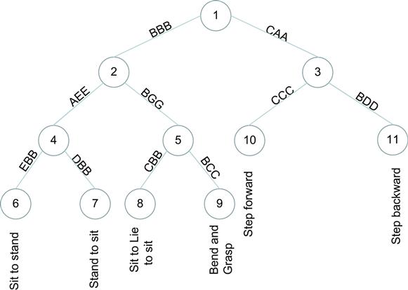
Once the Patricia tree is created, each leaf of the Patricia tree corresponds to a subset of the movements. During testing, the n-grams of the test trial are used to traverse the tree and return the corresponding movement set. The result may be an empty set or it may contain one or more movements. Specifically, if not enough n-grams are present to traverse the tree to a leaf, the algorithm returns all movements assigned to the leafs of the subtree rooted at the node where the traversal terminated. For example, in Figure 5 if the traversal would terminate at Node2, then the set containing {Sit to Stand, Stand to Sit, Sit to Lie to Sit, Bend and Grasp} is reported as the answer. If the traversal would terminate at Node5, then only the set containing {Sit to Lie to Sit, Bend and Grasp} is reported. Finally, if the traversal terminates at a leaf Node1, then the system reports only Step Backward as the answer.
7 Data-Mining Model
Based on the constructs defined earlier, a data-mining approach is proposed for BSN data. The approach has two distinct parts: training and query processing.
7.1 Training
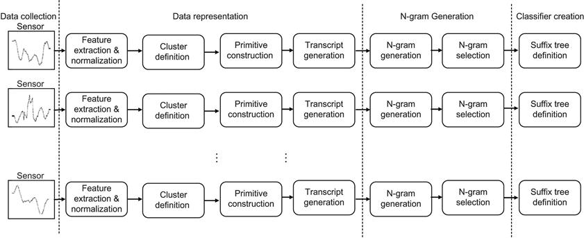
During the training phase of the execution, the system acquires parameters that can be used during the query processing. The training starts with selecting a portion of the available data trials for training. First and second derivatives are then extracted from each one of the trials for every sensing axis. Features are then normalized with respect to each subject using a standard score (or z-score) [48] in order to remove intersubject variations of the same movements. Then normalized features are used to define data clusters as described in section 4.1. Once the data clusters are defined, primitives are extracted for the data points in each training trial and then combined to define motion transcripts as described in section 4.2. The next step is to extract n-grams from each one of the transcripts generated for the training samples. Since the number of n-grams is very large, the system then selects a small number of t n-grams using the information gain as described in section 5.1. Finally, the system constructs a Patricia tree with selected n-grams on the edges and movement classes on the leafs as described in section 6. The overall process is demonstrated in Figure 6. The parameters defined during the training are data clusters for each sensing axis, n-grams selected with respect to the IG criteria, and the Patricia trees for classification. Clusters are represented by the cluster center coordinates, while important features selected for each sensing axis of each mote are then combined and stored.
7.2 Query Processing
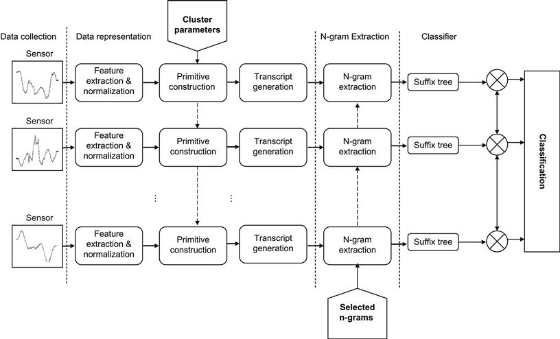
When the system needs to search for a query or a movement, it receives input in the form of the sensor readings. First and second derivatives are extracted from the sensor readings of each of the sensing axes. Based on these features and clusters, defined during the training of the system, each data point of the trial is labeled with a primitive. Primitives are combined with respect to timing alignment into motion transcripts. The system then traverses the transcript of the trial and verifies if it contains important n-grams selected during the training. Using this information, the system traverses the Patricia tree defined for this sensing axis during the training and returns the set of movements assigned to the leaf where the traversal terminated. If the traversal terminated at node p that is not a leaf, the algorithm returns all the movements assigned to the leafs of the subtree rooted at node p. This allows the system to avoid introducing bias for the axis that observes the same signal for two different movements. Since all these operations are defined in terms of the individual sensing axis, an approach is required to combine the local decisions. A simple voting scheme is used, which performs well in the context of this dataset. However, this method can be improved by treating each sensory axis as an individual classifier. To determine the final decision, the individual classifiers can be combined in an intelligent way such as AdaBoost [58]. The flow of the query processing is demonstrated in Figure 7.
Because the system initially processes each sensing axis individually, it is possible to query only for a subset of axes available in the system. This can be useful when a specific sensor is not available to all users. For example, one user can use a three-dimensional gyroscope, while another may use only a two-dimensional gyroscope. Additionally, since the system uses a voting scheme, it is possible to make classification decisions based on the local view of only a subset of nodes.
8 Experimental Results
To verify the performance of the proposed data-mining approach, it was applied to a pilot application discussed in section 3.3. The verification step was split into two phases. The first phase involved locating the correct place in the repository to store the signal for an unknown trial. To achieve this, the available data was split into two equal sets. The first half of the data was used to train the system, while the second half of the data was used to verify the classification accuracy. The second phase was used to create a representative signal template for each movement, searching the entire repository for the trials consistent with the template.
Initially the data-mining algorithm was trained on the entire data set. During the training, the algorithm selects n-gram sets, or templates, specific to each movement. The individual templates are then used to search for relevant trials in the entire repository. While evaluating the results, the results of classification when k-Means clustering is used are compared to the results when GMM clustering is used. The accuracy of the approach is considered with respect to the length of the n-gram n and number of features selected t. Finally, the accuracy trade-off is demonstrated with respect to n and t. For the second part of the analysis, the average frequency of the template appearance in the repository is assessed. The computed templates are then considered in the context of individual trials. If a trial contains enough n-grams from a given template, it is accepted as the movement represented by that template. Otherwise, the trial is rejected. The accuracy of trial classification is reported for each of the movement templates.
8.1 k-Means or GMM?
The movement transcript generated based on the k-Means and GMM clustering was used to compare two clustering approaches for a 3-gram with the number of selected n-grams varying from 1 to 6 per sensing axis as shown in Table 3, and with {1..6}-gram with only 1 n-gram selected from each sensing axis as shown in Table 4. Both tables indicate that an increase in t or n would increase the precision and recall for both approaches until the over-fitting point is reached. It is also clear that the GMM approach outperforms the k-Means approach with respect to varying both n and k, and therefore is a better candidate for the example application.


8.2 Classification Accuracy
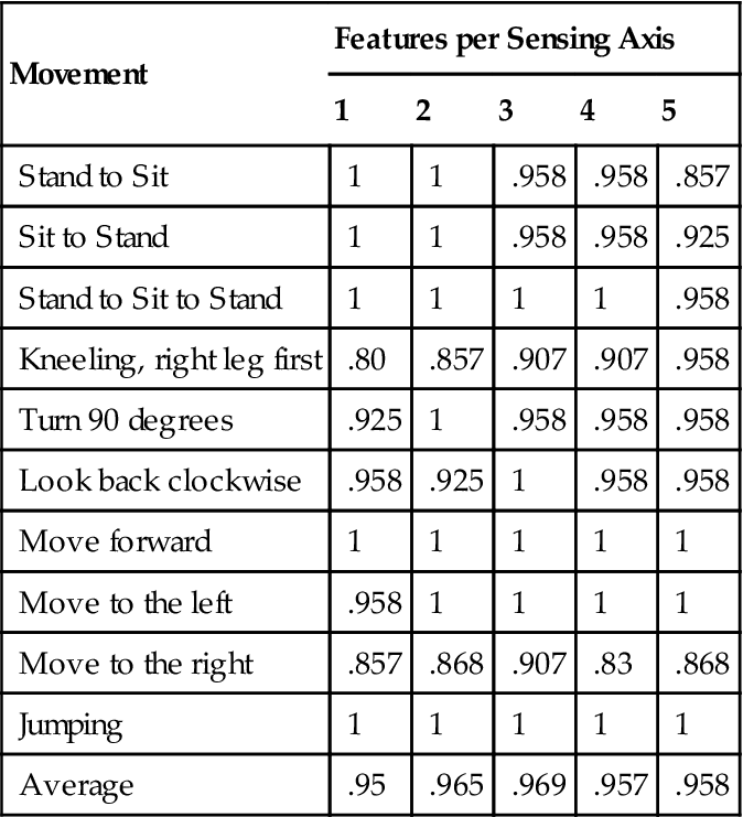
To evaluate classification accuracy, the precision and recall of movement classification were evaluated using the n-gram size of n=3 and number of features t={1, 2…5} with the GMM clustering model. Half of the dataset was used to train the system, while the other half was used to test it. The results of the classification are demonstrated in Table 5. The table contains the F-score defined as (2×P×R)/(P+R), where P is the classification precision and R is the classification recall. This table confirms that adding more n-grams would improve both average precision and average recall until an over-fitting point is reached. Note that individual values for movements sometimes decrease when an additional feature is selected. This is due to the fact that the data set has a considerable amount of noise, and while an n-gram improves the overall classification accuracy, it may cause confusion in classification of some trials where it appears as noise and not an important transition. Table 5 displays the number of n-grams extracted from each sensing axis, so the total number of the n-grams extracted by a sensor node should be multiplied by 5. However, even after that, the classification accuracy is fairly high for the number of features considered.
Table 5
Classification Precision with Respect to the Number of Features Selected
| Movement | Features per Sensing Axis | ||||
| 1 | 2 | 3 | 4 | 5 | |
| Stand to Sit | 1 | 1 | .958 | .958 | .857 |
| Sit to Stand | 1 | 1 | .958 | .958 | .925 |
| Stand to Sit to Stand | 1 | 1 | 1 | 1 | .958 |
| Kneeling, right leg first | .80 | .857 | .907 | .907 | .958 |
| Turn 90 degrees | .925 | 1 | .958 | .958 | .958 |
| Look back clockwise | .958 | .925 | 1 | .958 | .958 |
| Move forward | 1 | 1 | 1 | 1 | 1 |
| Move to the left | .958 | 1 | 1 | 1 | 1 |
| Move to the right | .857 | .868 | .907 | .83 | .868 |
| Jumping | 1 | 1 | 1 | 1 | 1 |
| Average | .95 | .965 | .969 | .957 | .958 |
8.3 Parameter Trade-offs
The classification accuracy in the proposed data-mining approach depends on two parameters: the length of the substring n and the number of n-grams t selected for classification. As t is increasing, so does the accuracy until the over-fitting point is reached. After the over-fitting point is reached, the accuracy of the approach will no longer improve with additional features. It is clear that a large n inherently is able to capture more structural information. However, since a moving window is used for n-gram extraction, a single erroneous primitive affects more n-grams for larger values of n, which is equivalent to experiencing the over-fitting sooner. The algorithm is expected to converge to the best accuracy faster for large values of n, but it also means that the over-fitting point will happen faster. Table 6 demonstrates the F-score of accuracy vs. the number of n-grams t for different values of n.
Table 6
Precision with Respect to n-Gram Size and Number of n-Grams Selected
| n | Features per Sensing Axis | ||||
| 1 | 2 | 3 | 4 | 5 | |
| 3 | .95 | .97 | .97 | .96 | .95 |
| 5 | 1 | .97 | .97 | .99 | .98 |
| 7 | .99 | .99 | .99 | .98 | 1 |
| 9 | .98 | .97 | .97 | .97 | .96 |
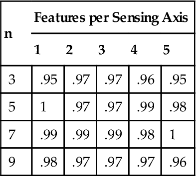
From the tables, it is clear that higher values of n are desirable before over-fitting, which means that n should be determined based on the expected amount of noise in the original signal. For a lower amount of noise, a higher value of n would work better, while when the amount of noise is larger, lower values of n will provide a safer solution with less risk of over-fitting. In this example, the precision is improving from n=3 to n=5, it is fairly stationary from n=5 to n=7, and finally, at n=9 has decreasing performance. The fact that larger n-grams take more time to locate in the training trials should also be considered. The system can evaluate multiple possibilities during the training and generate the curves to identify the best operational point from the perspective of accuracy and speed trade-offs.
8.4 Movement Template Evaluation
Based on the parameters selected in section 8.3, Ti is defined as the combination sets of 3-grams selected for each sensing axis during the training process for movement Mi. Here the entire data set is used to train the templates. Once the training is complete and the templates are generated, the average quality measure is evaluated for each Ti. It is done by checking how often the n-grams of each Ti appear in movement trials of every movement. Intuitively, n-grams of Ti should appear more often in Mi than any other movement in order for the template to be effective. Table 7 demonstrates the results of this evaluation normalized with respect to the size of each template, meaning that on average, 51% of T1 appear in trials of M1, while only 36% of T1 appear in trials of M2.
Table 7
Average Template Evaluation Normalized with Respect to the Template Size
| Ti | Movement | |||||||||
| 1 | 2 | 3 | 4 | 5 | 6 | 7 | 8 | 9 | 10 | |
| 1 | .51 | .36 | .4 | .37 | .32 | .29 | .37 | .35 | .34 | .22 |
| 2 | .33 | .49 | .34 | .37 | .33 | .27 | .42 | .38 | .41 | .29 |
| 3 | .39 | .41 | .54 | .42 | .30 | .29 | .37 | .34 | .36 | .33 |
| 4 | .22 | .23 | .27 | .57 | .37 | .21 | .37 | .31 | .36 | .27 |
| 5 | .25 | .28 | .24 | .36 | .55 | .28 | .35 | .37 | .4 | .31 |
| 6 | .42 | .40 | .4 | .44 | .46 | .56 | .46 | .46 | .47 | .26 |
| 7 | .23 | .25 | .21 | .4 | .35 | .24 | .66 | .42 | .5 | .26 |
| 8 | .31 | .3 | .25 | .33 | .33 | .26 | .43 | .61 | .40 | .23 |
| 9 | .27 | .27 | .23 | .39 | .35 | .26 | .48 | .41 | .59 | .25 |
| 10 | .23 | .25 | .23 | .27 | .24 | .18 | .26 | .26 | .27 | .57 |

Two observations can be made based on the results in Table 7. First, it is clear that n-grams of Ti appear most often in the Mi itself. This observation is in line with the expectation for a good template. While n-grams of the Ti , on average, appear 10% more often in the respective Mi , they also appear in trials of other movements with a sizable number of occurrences. These results suggest that a closer look on a per-trial basis is required to evaluate the template quality. The intuitive approach to this problem is to search for trials that have the entire template present. However, in a realistic system with noisy trials, this solution is not practical, since it’s unlikely that many trials will be perfect. Table 7 confirms this: the highest average values for each Ti are close to 50% and not 100%. This problem is solved by introducing a variable α, which defines the proportion of the number of n-grams from a Ti that need to be present in a trial for it to be classified as Mi. If the α value is too low, it is likely that some trials will be erroneously identified as Mi, increasing the number of false positives and decreasing the precision of the template. However, if the α value is too high, some trials of Mi will not be identified, increasing the amount of false negative errors and decreasing the recall of the template. Additionally, lower values of α can speed up the computation, which is desirable in our problem due to a potentially large number of movements in the repository. To achieve a balance between the precision and recall, as well as to promote faster data mining, the value of α=.5 is selected. The value of 50% is also suggested by Table 7, where the average presence of more than 50% n-grams from a template Ti identifies the movement Mi associated with that template. Table 8 demonstrates the normalized number of trials of each movement identified as Mi by each of the templates Ti, meaning, for example, that template T1 selects 78% of trials belonging to M1.
Table 8
Template Evaluation for Individual Trials Normalized with Respect to the Number of Trials of Each Movement
| Ti | Movement | |||||||||
| 1 | 2 | 3 | 4 | 5 | 6 | 7 | 8 | 9 | 10 | |
| 1 | .48 | 0 | 0 | 0 | 0 | 0 | 0 | 0 | 0 | 0 |
| 2 | 0 | .41 | 0 | 0 | 0 | 0 | 0 | 0 | 0 | 0 |
| 3 | 0 | 0 | .78 | .03 | 0 | 0 | 0 | 0 | 0 | 0 |
| 4 | 0 | 0 | 0 | .96 | 0 | 0 | 0 | 0 | 0 | 0 |
| 5 | 0 | 0 | 0 | 0 | .93 | 0 | 0 | 0 | 0 | 0 |
| 6 | 0 | 0 | 0 | .18 | .18 | .89 | .14 | .14 | .22 | 0 |
| 7 | 0 | 0 | 0 | .03 | 0 | 0 | 1 | 0 | .44 | 0 |
| 8 | 0 | 0 | 0 | 0 | 0 | 0 | .07 | .96 | 0 | 0 |
| 9 | 0 | 0 | 0 | 0 | 0 | 0 | .22 | 0 | 1 | 0 |
| 10 | 0 | 0 | 0 | 0 | 0 | 0 | 0 | 0 | 0 | .96 |
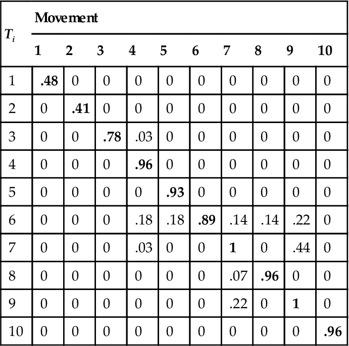
With α=.5, each Ti correctly identifies substantially more trials of its own movement than any other movement. This low value of α also defines a search speed increase of up to 50% since only 50% of the trials in templates need to be located. However, higher false negative and false positive errors are observed for certain templates, which suggests that a static value of α is inappropriate. Templates T1 and T2 do well at identifying only trials of their respective movements. However, less than half of the appropriate trials are identified. This suggests that the value of α=.5 is too high for these templates. At the same time, T6 and T7 have a much better rate of recognizing trials of their respective movements, but they also falsely identify trials of other movements. This suggests that the value of α=.5 is too low for these templates. Defining a movement-specific value of αi, based on the training set for each template can decrease the amount of errors in the system.
9 Conclusion and Recommendations
This chapter introduced a data-mining approach for a repository of movement data acquired by wearable sensors that can capture structural properties of the observed movements. This mining algorithm has the potential to significantly simplify the deployment and management of large data repositories since it removes the need for extensive per-subject training. The chapter demonstrated that the proposed approach has suitable performance on the pilot application and explored the trade-offs between the length of the extracted n-grams and the required number of features for the best classification results. While the results are promising, they can be improved in two ways. First, the performance of each component of the data-mining algorithm can be analyzed in detail and the implementation details may be modified for enhancing the performance and reducing the computational complexity. Second, in order to group similar movements together, the approach relies on the fact that similar sensor placement will be used.
It is a strong assumption, granted that for the inertial MEMs sensors even a small misplacement may result in changes in the sensor output. Furthermore, it is likely that during longer periods of sensor deployment, sensors can become loose or misplaced. Advanced data-mining techniques may help with slight orientation changes or displacement; however, the change may become significant with time, and the data for a given subject may become less similar to the original training data from the repository. There are two possible directions that can be taken to address this issue. The proposed data-mining approach needs to be evaluated with respect to the sensor misplacements. This step will clarify the question of ”how much displacement is too much?” and will lay the foundation for tracking and compensation of the sensor position and orientation. Tracking of the sensor displacement is challenging without an additional sensory perspective because all of the sensors considered so far collect data in the local frame of reference. Additional information can be extracted from supplementary modalities, e.g., cameras or other types of wearable sensors. These additional modalities can be used to track changes in orientation, and an intelligent algorithm can be developed to continuously calibrate the motion sensors. For example, a camera available at home can be used to calibrate motion sensors every time a user passes by. These periodic calibrations will guarantee consistent system performance.
The pilot application introduced in this chapter demonstrates the behavior of the proposed mining approach based on the example of inertial wearable sensors. The same idea will apply to other types of wearable sensors; for example, ECG or GSR sensors can be analyzed in a similar fashion. To do that, the reader will need to follow the conceptual steps outlined in this chapter. First, extract features from the raw sensor signal that highlight the structural properties of the data for a given application. Then use the extracted features to create signal transcripts. Finally, execute the proposed mining approach with signal transcripts as an input. Note that other applications can have limitations that were not considered in this chapter.
Acknowledgment
This work was supported in part by the National Science Foundation, under grant CNS-1150079. Any opinions, findings, conclusions, or recommendations expressed in this material are those of the authors and do not necessarily reflect the views of the funding organizations.