
Computing receiver noise and SNR at a receiver is important for determining coverage and quality of service in a wireless communication system.
As shown in Chapters 3, 6, and 7, SNR determines the link quality and impacts the probability of error in a wireless communication system. Thus, the ability to estimate SNR is important for determining suitable transmitter powers or received signal levels in various propagation conditions.
The signal level at a receiver antenna may be computed based on path loss equations given in Chapters 3 and 4. To compute the noise level of a receiver, it is necessary to know the gains (or losses) of each receiver stage, as well as the ambient noise temperature at the receiver antenna. However, the noise figure of a receiver is a convenient metric that allows a designer to factor in the additional noise induced by the receiver without having to know about the specific components that make up the receiver stages.
All electronic components generate thermal noise, and hence contribute to the noise level seen at the detector output of a receiver. In order to refer the noise at the output of a receiver to an equivalent level at the receiver input terminals (where the signal is applied), the concept of noise figure is used [Cou93]. By referring noise levels to the receiver input, one merely needs to add the noise figure of the receiver to the ambient thermal noise level in order to model the total noise power at the receiver input terminals.
Noise figure, denoted by F, is defined as
F is always greater than 1 and assumes that a matched load operating at room temperature is connected to the input terminals of the device. A noise figure of 1 implies a noiseless device.
Noise figure may be related to the effective noise temperature, Te, of a device by
where T0 is ambient room temperature (typically taken as 290 K to 300 K, which corresponds to 63°F to 75°F, or 17°C to 27°C). Noise temperatures are measured in Kelvin, where 0 K is absolute zero, or −273°C. A noiseless device has Te = 0 K.
Note that Te does not necessarily correspond to the physical temperature of a device. For example, directional satellite dish antennas which beam toward space typically have effective antenna temperatures on the order of 50 K (this is because space appears cold and produces little in the way of thermal noise), whereas a 10 dB attenuator has an effective temperature of about 2700 K (this follows from Equations (B.2) and (B.4)). Antennas which beam toward earth generally have effective noise temperatures which correspond to the physical temperature of the earth, which is about 290 K.
A simple passive load (such as a resistor) at room temperature transfers a noise power of
into a matched load, where k is Boltzmann’s constant given by 1.38 × 10⁻²³ Joules/Kelvin and B is the equivalent bandwidth of the measuring device. For passive devices such as transmission lines or attenuators operating at room temperature, the device loss (L in dB) is equal to the noise figure of the device. That is,
For the purposes of noise calculations, antennas which are built with passive elements (such as wire) are considered to have unity gain, even if their radiation pattern has a measured gain.
The concepts of noise figure and noise temperature are useful in communications analysis, since the gains of the receiver stages are not needed in order to quantify the overall noise amplification of the receiver. If a resistive load operating at room temperature is connected to the input terminals of a receiver having noise figure F, then the noise power at the output of the receiver, referred to the input, is simply F times the input noise power, or
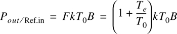
and the actual noise power out of the receiver is
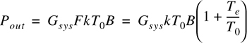
where Gsys is the overall receiver gain due to cascaded stages.
For a cascaded system, the noise figure of the overall system may be computed from the noise figures and gains of the individual components. That is,
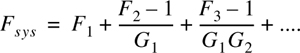
or equivalently
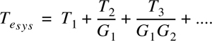
where gains are in absolute (not dB) values. The following examples illustrate how to compute the noise figure of a mobile receiver station, and consequently the average receiver noise floor that is used in a link budget.
Example B.1.
If a wireless link provides an SNR of 20 dB to the receiver antenna input terminals, and the receiver is specified to have a noise figure of 6 dB, what is the SNR at the detector output stage of the receiver?
Solution
Using the concept of noise figure, it is easy to compute the SNR at the detector stage from Equation (B.5).
Since the receiver amplifies the signal and the noise by the same factor, and the noise out is F times the noise in, then
or, in dB values, SNROUT = SNRIN − F.
Thus, for this example,
SNROUT(dB) | = | 20 – 6 |
SNROUT(dB) | = | 14 dB |
The output SNR is equal to 14 dB, even though the input SNR is 20 dB.
Example B.2.
Consider an AMPS cellular phone with a 30 kHz RF equivalent bandwidth. The phone is connected to a mobile antenna as shown in Figure B.2. If the noise figure of the phone is 6 dB, the coaxial cable loss is 3 dB, and the antenna has an effective temperature of 290 K, compute the noise figure of the mobile receiver system as referred to the input of the antenna terminals.
To find the noise figure of the receiver system, it is necessary to first find the equivalent noise figure due to the cable and AMPS receiver. Note that 3 dB loss is equal to a loss factor of 2.0. Using Equation (B.4), which indicates that the cable has a noise figure equal to the loss, and keeping all values in absolute (rather than dB) units, the receiver system has a noise figure given by Equation (B.7)
Example B.3.
For the receiver in Figure B.2, determine the average output thermal noise power, as referred to the input of the antenna terminals. Assume To = 300 K.
Solution
From Example B.2, the cable/receiver system has a noise figure of 9 dB. Using Equation (B.2), the effective noise temperature of the system is
Te = (8–1)300 = 2100K |
Using Equation (B.8), the overall system noise temperature due to the antenna is given by
Ttotal = Tant + Tsys = (290+2100)K = 2390 K |
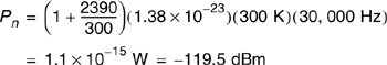
Now using the right-hand side of Equation (B.5), the average output thermal noise power referred to the antenna terminals is given by
Example B.4.
For the receiver in Figure B.2, determine the required average signal strength at the antenna terminals to provide a SNR of 30 dB at the receiver output.
Solution
From Example B.3, the average noise level is −119.5 dBm. Therefore, the signal power must be 30 dB greater than the noise
Ps (dBm) = SNR + (−119.5) = 30 + (−119.5) = −89.5 dBm. |