
This Appendix derives the three rate variance relationships presented in Chapter 5.
The power spectral density (PSD) of a baseband complex received voltage signal is related to the angular distribution of multipath power [Gan72]:
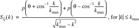
where θ is the azimuthal direction of travel and p(·) is the angular distribution of impinging multipath power. The value kmax is the maximum wavenumber, which is equal to 2π/λ. Note that the PSD is a function of wavenumber, k, instead of frequency, ω, since multipath angles-of-arrival directly relate to spatial selectivity. By extension, the PSD is identical to the Doppler Spectrum,![]() , of a mobile receiver if the receiver moves in a static channel.
, of a mobile receiver if the receiver moves in a static channel.
The second moment of the fading process is given by the following integration [Jak74]:
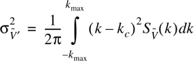
where kc is the centroid of the PSD:

F0 is defined by Equation (5.90)—this is really just the average power of the process.
Now insert Equation (C.3) into Equation (C.2), making the change of variable θx = θ ± cos–1 (k/kmax), where the + and − signs correspond to the left and right terms of p(·), respectively, of Equation (C.1). After rearranging the limits of integration, the equation for ![]() , becomes
, becomes

Consider a complex Fourier expansion of ![]() with respect to θ:
with respect to θ:

All of the An are zero for odd n. This is because ![]() ; that is, a 180° change in the direction of mobile travel should produce identical statistics. Furthermore, Equation (C.4) has no harmonic content with respect to θ for n > 2. Solving for the only two remaining complex coefficients produces
; that is, a 180° change in the direction of mobile travel should produce identical statistics. Furthermore, Equation (C.4) has no harmonic content with respect to θ for n > 2. Solving for the only two remaining complex coefficients produces

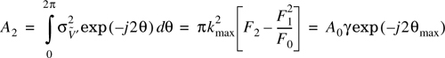
where Λ, γ, and θmax, are the three basic spatial channel parameters defined in Equations (5.91)–(5.93). If these two coefficients are placed back into Equation (C.5), the end result is the relationship for ![]() in Equation (5.94).
in Equation (5.94).
For a mobile receiver, it is often convenient to measure the fading rate variance in terms of change per unit time instead of distance. If the mobile receiver operates in an otherwise static channel, then the mean-squared time rate-of-change, ![]() , is equal to
, is equal to ![]() multiplied by the squared velocity of the receiver.
multiplied by the squared velocity of the receiver.
The stochastic process of power is defined as ![]() . Thus, the PSD of power for k ≠ 0 is the convolution of two complex voltage PSDs:
. Thus, the PSD of power for k ≠ 0 is the convolution of two complex voltage PSDs: ![]() , provided the complex voltage,
, provided the complex voltage, ![]() , is a Gaussian process (the condition for Rayleigh fading) [Pap91]. The rate variance relationship for power may then be written as
, is a Gaussian process (the condition for Rayleigh fading) [Pap91]. The rate variance relationship for power may then be written as


Making the substitution k = λ-k′ leads to

which may be regrouped and re-expressed in terms of the spectral centroid, kc:

Now simply substitute Equation (5.94) for ![]() , to obtain Equation (5.95).
, to obtain Equation (5.95).
Based on the power relationship P(r) = R2(r), it is possible to write the following:
which is valid for a Rayleigh fading process since R and its derivative are independent [Ric48]. Setting the left-hand side of Equation (C.12) equal to the rate variance relationship for power in Equation (5.95) produces the mean-squared fading rate result for a Rayleigh-fading voltage envelope in Equation (5.96).