
This Appendix contains detailed mathematical analysis which provides expressions for determining the average bit error rate for users in a single channel, CDMA, mobile radio system. Using the expressions provided in this appendix, it is possible to analyze CDMA systems for a wide range of interference conditions. These expressions may be used to reduce or eliminate the need for time intensive simulations of CDMA systems in some instances.
In a spread spectrum, Code Division Multiple Access (CDMA) system using binary signaling, the radio signal received at a base station from the kth mobile user (assuming no fading or multipath) is given by [Pur77]
where bk(t) is the data sequence for user k, ak(t) is the spreading (or chip) sequence for user k, τk is the delay of user k relative to some reference user 0, Pk is the received power of user k, and φk is the carrier phase offset of user k relative to a reference user 0. Since τk and φk are relative terms, we can define τ0 = 0 and φ0 = 0.
Both ak(t) and bk(t) are binary sequences with values −1 and +1. The cyclical pseudo noise (PN) chip sequence ak(t) is of the form

where M is the number of chips sent before the PN sequence repeats itself, Tc is the chip period, MTc is the repetition period of the PN sequence, Π(t) represents the unit pulse function, and i is an index to denote the particular chip within a PN chip cycle.
For the user data sequence, bk(t), Tb is the bit period. It is assumed that the bit period is an integer multiple of the chip period such that Tb = NTc. Note that M and N are not necessarily equal. In the case where they are equal, the PN sequence is repeated for every bit period. The user data sequence bk(t) is given by

In a mobile radio, spread spectrum, CDMA system, the signals from many users arrive at the input of the receiver. A correlation receiver is typically used to “filter” the desired user from all other users which share the same channel.
At the receiver, illustrated in Figure E.1, the signal available at the input to the correlator is given by

where n(t) is additive Gaussian noise with two-sided power spectral density N0/2. It is assumed in Equation (E.5) that there is no multipath in the channel with the possible exception of multipath that leads to purely flat, slow fading.

The received signal contains both the desired user and (k – 1) undesired users and is mixed down to baseband, multiplied by the PN sequence of the desired user (user 0, for example), and integrated over one bit period. Thus, assuming that the receiver is delay and phase synchronized with user 0, the decision statistic for user 0 is given by:

For convenience and simplicity of notation, the remainder of this analysis considers bit 0 (j = 0 in (E.6)).
Substituting Equations (E.1) and (E.5) into Equation (E.6), the decision statistic of the receiver is found to be

where I0 is the desired contribution to the decision statistic from the desired user (k = 0), ζ is the multiple access interference from all co-channel users (which may be in the same cell or in a different cell), and η is the thermal noise contribution.
The contribution from the desired user is given by

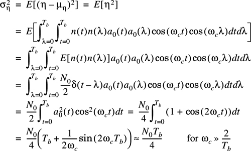
The noise term, η, is given by:

It is assumed that n(t) is white Gaussian noise with two-sided power spectral density N0/2. The mean of η is

and the variance of η is
The third component in Equation (E.8), ζ, represents the contribution of multiple access interference to the decision statistic. ζ is the summation of K – 1 terms, Ik,

each of which is given by

It is useful to simplify Equation (E.14) in order to examine the effects of multiple access interference on the average bit error probability for a single user (i.e., user 0 for simplicity). The relationship between bk(t − τk), ak(t − τk), and a0(t) is illustrated in Figure E.2.

The quantities γk and Δk in Figure E.2 are defined from the delay of user k relative to user 0, τk, such that [Pur77]
The contribution from kth, interfering user, to the decision statistic is given by [Pur77], [Mor89b]

where Xk, Yk, Uk, and Vk have distributions, conditioned on A and B, which are given by:


It is useful to express Equation (E.16) in a way that exploits knowledge of the statistical properties of the signature sequence to determine the impact of multiple access interference on the bit error rate of a particular desired user (as shown in [Leh87][Mor89b]). This leads to the derivation of Equations (E.17)–(E.20).
To derive Equations (E.17)–(E.20), assume that the chips are rectangular, and refer to Figure E.2. The integration of Equation (E.16) may be rewritten as

It is convenient to rewrite this as

This may be rearranged to give [Leh87]

Lehnert defined random variables Zk, l as [Leh87]

where each of the Zk, j are independent Bernoulli trials, equally distributed on {−1, 1}.
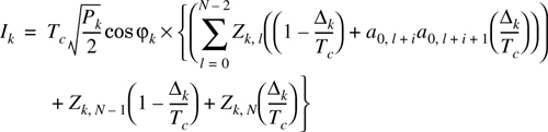
Then, using Equation (E.24) and the fact that ![]() , Equation (E.23) may be expressed as
, Equation (E.23) may be expressed as
Let ![]() be the set of all integers in [0, N – 2] for which
be the set of all integers in [0, N – 2] for which ![]() . Similarly, let
. Similarly, let ![]() be defined as the set of all integers in [0, N – 2] for which
be defined as the set of all integers in [0, N – 2] for which ![]() . Then, Equation (E.25) may be expressed as
. Then, Equation (E.25) may be expressed as

Now define


Note that {Zk, l} is a set of independent Bernoulli trials [Coo86], each with each outcome identically distributed on {−1, +1}. If we let A denote the number of elements in the set ![]() and let B denote the number of elements in the set
and let B denote the number of elements in the set ![]() , then the probability density functions for Xk and Yk are given by
, then the probability density functions for Xk and Yk are given by


and the quantities Uk and Vk are each distributed as


Thus, the interference contributed to the decision statistic by a particular multiple access interferer is entirely defined by the quantities Pk, φk, Δk, A, and B as given in Equations (E.16)–(E.20). Note that A and B are solely dependent on the sequence of user 0. Furthermore, A + B = N − 1, since sets ![]() and
and ![]() are disjoint and span the set of total possible signature sequences of length N in which there are a total of N – 1 possible chip level transitions.
are disjoint and span the set of total possible signature sequences of length N in which there are a total of N – 1 possible chip level transitions.
The use of the Gaussian Approximation to determine the bit error rate in binary, CDMA, multiple access, communication systems is based on the argument that the decision statistic, Z0, given by Equation (E.8), may be modeled as a Gaussian random variable [Pur77], [Mor89b]. The first component in Equation (E.8), I0, is deterministic, and its value is given by Equation (E.9). The other two components of Z0 (i.e., ζ and η), are assumed to be zero-mean Gaussian random variables. Assuming that the additive receiver noise, n(t), is bandpass Gaussian noise, then η, which is given by Equation (E.10), is a zero-mean Gaussian random variable. This section derives an expression for the bit error rate based on the assumption that the multiple access interference term, ζ, may be approximated by a Gaussian random variable.
First define a combined noise and interference term ξ, given by
such that the decision statistic, Z0, is given by
where Z0 is a Gaussian random variable with mean I0 and a variance which is equal to the variance, ![]() of ξ.
of ξ.
The probability of error in determining the value of a received bit is equal to the probability that ξ < – I0 when I0 is positive and ξ > I0 when I0 is negative. Due to its structure, ξ is symmetrically distributed such that these two conditions occur with equal probability, therefore we may say that the probability of error is equal to the probability that ξ > |I0|. If ξ is a zero-mean Gaussian random variable with variance, ![]() , the probability of a bit error is given by
, the probability of a bit error is given by

where the Q function is defined in Appendix F. Using Equation (E.9), this may be rewritten as:

Assuming that the multiple access interference contribution to the decision statistic, ζ, can be modelled as a zero-mean Gaussian random variable with variance ![]() , and that the noise contribution to the decision statistic, η, may be modelled as a zero-mean Gaussian noise process with variance
, and that the noise contribution to the decision statistic, η, may be modelled as a zero-mean Gaussian noise process with variance ![]() , then it follows that since the noise and the multiple access interference are independent, the variance of ξ is given simply by
, then it follows that since the noise and the multiple access interference are independent, the variance of ξ is given simply by
All that remains is to justify the Gaussian approximation for ζ, and to determine the value of ![]() .
.
Using Equations (E.13) and (E.16), the total multiple access interference contribution to the decision statistic for user 0, is given by

which may be expressed as

where

The exact distributions for Xk and Yk are given by Equations (E.17) and (E.18) and the distributions of Uk and Vk are given in Equations (E.19) and (E.20). Note that Wk may only take on discrete values (a maximum of (N − 1) B − B2 + 6 values) for a given Δk.
The Central Limit Theorem (CLT) [Sta86], [Coo86] is used to justify the approximation of ζ as a Gaussian random variable. The CLT considers the normalized sum of a large number of identically distributed random variables xi, where y is the normalized random variable given by

and each xi has mean μ and variance σ2. The random variable y is approximately normally distributed (a Gaussian distribution with zero mean and unit variance) as M becomes large. To justify the Gaussian approximation when the interferer power levels are not equal or not constant, a more general definition of the CLT is required as given by Stark and Woods [Sta86].
This more general statement of the CLT [Sta86], requires that the sum

of M random variables, xi (which are not necessarily identically distributed but are independent), each with mean μxi and variance ![]() , approaches a Gaussian random variable as M gets large, provided that
, approaches a Gaussian random variable as M gets large, provided that

Furthermore, the mean and variance of the sum, y, are given by


The condition for Equation (E.45) to hold is equivalent to specifying that no single user dominates the total multiple access interference.
Consider the statistics of ζ conditioned on a specific set of operating conditions, namely, the set of K – 1 delays {Δk}, K – 1 phase shifts {φk}, K – 1 received power levels {Pk}, and the number of chip transitions during on complete cycle of the PN sequence for user 0.
It can be shown that each of the multiple access interferers are uncorrelated given a particular set of operating conditions [Leh87]:

The terms Xk, Yk, Uk, and Vk in Equation (E.42) are uncorrelated, so that

Noting that the random variables Uk and Vk take on values of {−1, +1} with equal probability, therefore ![]() and
and ![]() , and it follows that
, and it follows that

where Xk is the summation of A independent and identically distributed Bernoulli trials, xi, each with equally likely outcomes from {−1, +1}. In Equation (E.31), A is the number of possible values of l such that the bit patterns ![]() for l ε [0, N − 2] and i is the offset of first chip of the detected bit relative to the start of the PN sequence. Now, solving for E[Xk|B]
for l ε [0, N − 2] and i is the offset of first chip of the detected bit relative to the start of the PN sequence. Now, solving for E[Xk|B]

where B is the number of bit transitions, i.e., the values of l such that the bit patterns ![]() . Similarly for Yk,
. Similarly for Yk,

Therefore, Equation (E.50) may be rewritten

Using Equation (E.48)
Taking the expected value of Equation (E.54) over Δk and φk on a chip interval yields

Finally, assuming random signature sequences for each user, and averaging Equation (E.55) over B with E[B] = (N − 1)/2, the variance of the total multiple access interference conditioned on the received power level, Pk is found to be

If the set of power levels for the K − 1 interfering users are constant, then

If the K − 1 values of ![]() satisfy Equation (E.45), then ζ, will be a zero-mean Gaussian random variable as K − 1 gets large. The variance of ζ is given by
satisfy Equation (E.45), then ζ, will be a zero-mean Gaussian random variable as K − 1 gets large. The variance of ζ is given by

Therefore the decision statistic Z0 of Equation (E.36) may be modeled as a Gaussian random variable with mean given by Equation (E.9) and variance given by Equation (E.39)

Therefore, from Equation (E.38), the average bit error probability is given by

In typical mobile radio environments, communication links are interference-limited and not noise-limited. For the interference-limited case,  , and the average bit error probability is given by

In the noninterference limited case, for perfect power control where Pk = P0 for all k = 1... K − 1,

Finally, in the interference limited case with perfect power control, Equation (E.62) may be approximated by

Note that in Equation (E.60), the bit error rate is evaluated assuming that variance of the multiple access interference assumes its average value. In Section E.2, an alternative expression for the bit error rate is presented in which the bit error rate expression is averaged over the possible operating conditions, rather than evaluated at the average operating condition.
The expressions in Section E.1 are only valid when the number of users, K, is large. Furthermore, depending on the distribution of the power levels for the K – 1 interfering users, even when K is large, if Equation (E.45) is not satisfied, ζ will not be accurately modelled as a Gaussian random variable.
In situations where the Gaussian Approximation of Section E.1 is not appropriate, a more in-depth analysis must be applied. This analysis defines the interference terms Ik, conditioned on the particular operating condition of each user. When this is done, each Ik becomes Gaussian for large K. Define ψ as the variance of the multiple access interference for a specific operating condition:
First note that the conditional variance of the multiple access interference, ψ, is itself a random variable which is conditioned on the operating conditions {φk}, {Δk}, {Pk}, and B. In Equation (E.60), the bit error rate is evaluated assuming that the variance of the multiple access interference takes on its average value. Rather that evaluating Equation (E.37) for the average value of ψ, if the distribution of ψ is known, the bit error rate may be found by averaging overall possible values of ψ. This is given by

From Equations (E.48) and (E.54)

where

and where

Since the Uk and Vk are identically distributed for all k, it is convenient to drop the subscripts to obtain


and it is easily shown that E[Z′] = E[UV] = E[U]E[V] = N / 3.
The distribution of U is given as [Mor00]
and the distribution of V is given by [Mor00] as

where ![]() .
.
The distribution of the product of U and V, denoted by Z′, is given by [Mor89b]

The distribution of Zk, conditioned on the received power Pk of the kth user is
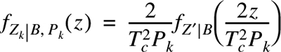
Letting ![]() and
and ![]() in Equation (E.75)
in Equation (E.75)

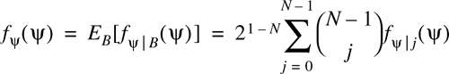
Since ψ is the summation of the K – 1 Zk terms, the probability density function for ψ is then given by the convolution
If the set of received powers, {Pk}, is fixed and nonrandom, then Equation (E.78) may be computed numerically by evaluating Equation (E.77) for each value of Pk. If the received power is a random variable, then an expression may be found for fψ(ψ) based on the distribution of power levels for the interfering users. Making the reasonable assumption that the power level for each user is identically and randomly distributed, then the distributions of the Zk terms are identical, such that ![]() . Then assuming that the distribution of the received interfering powers is known and given by some distribution fp(p) [Lib95]
. Then assuming that the distribution of the received interfering powers is known and given by some distribution fp(p) [Lib95]

in which case, Equation (E.78) reduces to
and the probability density function for the variance of the multiple access interference is given by
Equation (E.81) may be used in Equation (E.65) to determine the average bit error probability. This technique has been shown [Mor89b] to be accurate for a very small number of interfering users for the case of perfect power control.
Equation (E.65) assumes the interference-limited case. In general, when the noise term is significant

Thus, using Equations (E.76) and (E.79), the results of Morrow and Lehnert [Mor00] may be extended to include the case in which the power levels of the interfering users are constant but unequal and the case in which the power levels of the interfering users are independent and identically distributed random variables [Lib94a], [Lib95].
A Simplified Expression for the Improved Gaussian Approximation (SEIGA) [Lib95]
The expressions presented in Section E.2 are complicated and require significant computational time to evaluate. Holtzman [Hol92] presents a technique is for evaluating Equation (E.65) with (E.81) for the case of perfect power control. In addition, his results have been extended by Liberti [Lib94a] [Lib99] to treat the power levels of the K – 1 interfering users as independent and identically distributed random variables. This section also presents results for the case where the received power levels for the interfering users are constant but not identical (which is representative for very wideband CDMA systems).
The simplified bit error probability expressions are based on the fact that a continuous function f(x), may be expressed as
If x is a random variable and μ is the mean of x, then [Coo86]
where σ2 is the variance of x.
Further computational savings can be obtained by expanding in differences rather than derivatives, so that

which gives the approximation
In [Hol92], it is suggested that an appropriate choice for h is ![]() which yields
which yields
Using this approximation to evaluate Equation (E.65), the expression derived [Hol92] is found to be

where μψ is the mean of the variance of the multiple access interference, ψ, conditioned on a specific set of operating conditions, and ![]() is the variance of ψ. The conditional variance of the multiple access interference is given by Equation (E.66). If the received power levels from the K – 1 interfering users are identically distributed with mean μp and variance
is the variance of ψ. The conditional variance of the multiple access interference is given by Equation (E.66). If the received power levels from the K – 1 interfering users are identically distributed with mean μp and variance ![]() , then using the relationships in Equations (E.70)–(E.72), the mean and variance of ψ are given by
, then using the relationships in Equations (E.70)–(E.72), the mean and variance of ψ are given by

Using Equation (E.89), the variance of ψ is given by

where μp is the mean of the received power for each interfering user, and ![]() is the variance of the received power.
is the variance of the received power.
The expressions in Equations (E.89) and (E.90) were developed by Liberti [Lib94a] and are more general than the results originally given by Holtzman [Hol92], because they allow for the case in which the power levels of the interfering users are independent and identically distributed random variables.
Note that Equation (E.88) is only valid for ![]() to ensure that the denominator of the third term is positive. This leads to the following requirement
to ensure that the denominator of the third term is positive. This leads to the following requirement

Note that, in addition to limiting the ratio ![]() , Equation (E.91) bounds the lowest number of users K for which Equation (E.88) may be evaluated, since both
, Equation (E.91) bounds the lowest number of users K for which Equation (E.88) may be evaluated, since both ![]() and
and ![]() are positive. Examination of Equation (E.91) reveals that regardless of the values of
are positive. Examination of Equation (E.91) reveals that regardless of the values of ![]() and
and ![]() , for N ≥ 7, K must be greater than 2 to use Equation (E.88). For N < 7, K must be greater than 3. For most practical systems N ≥ 7 therefore a reasonable limitation is that Equation (E.88) may not be evaluated for the case of a single interfering user. Note that this is for the case of infinite signal-to-noise ratio. Later in this section, it is shown that for finite Eb/N0, the simplified expression for the Improved Gaussian Approximation may be used for K = 2 under certain conditions. Therefore, the Improved Gaussian Approximation (IGA) of Section E.2 should be used if the bit error probability is required for the case of K = 2, and for random powers, Equation (E.91) should be used to determine the minimum value of K which is allowed.
, for N ≥ 7, K must be greater than 2 to use Equation (E.88). For N < 7, K must be greater than 3. For most practical systems N ≥ 7 therefore a reasonable limitation is that Equation (E.88) may not be evaluated for the case of a single interfering user. Note that this is for the case of infinite signal-to-noise ratio. Later in this section, it is shown that for finite Eb/N0, the simplified expression for the Improved Gaussian Approximation may be used for K = 2 under certain conditions. Therefore, the Improved Gaussian Approximation (IGA) of Section E.2 should be used if the bit error probability is required for the case of K = 2, and for random powers, Equation (E.91) should be used to determine the minimum value of K which is allowed.
In cases for which Equation (E.91) is not satisfied, a value of h smaller than ![]() may be used in Equation (E.86). However, as h decreases, the simplified expression for the Improved Gaussian Approximation approaches the Gaussian Approximation of Equation (E.60) and, accordingly, it will become inaccurate for small numbers of users.
may be used in Equation (E.86). However, as h decreases, the simplified expression for the Improved Gaussian Approximation approaches the Gaussian Approximation of Equation (E.60) and, accordingly, it will become inaccurate for small numbers of users.
For the special case of perfect power control such that all users have identical power levels and these power levels are not random, Equation (E.90) may be used with ![]() . In particular, for
. In particular, for ![]() and
and ![]() with the chip period normalized to Tc = 1, Equations (E.89) and (E.90) yield the results presented by Holtzman [Hol92]:
with the chip period normalized to Tc = 1, Equations (E.89) and (E.90) yield the results presented by Holtzman [Hol92]:

For the case where the K – 1 interfering users have constant but unequal power levels, the mean and variance of ψ are given by


For the case of perfect power control with Pk = 2 for all k = 1...K – 1 and normalized Tc = 1, Equations (E.94) and (E.95) reduce to Equations (E.92) and (E.93), respectively. Finally, in the most general case, in which the received power from each user is a random variable with mean ![]() and variance
and variance ![]() , the mean and variance of ψ are given by
, the mean and variance of ψ are given by


The expressions given in Equations (E.94) through (E.97) generalize the results of Holtzman [Hol92] to the case in which the power levels of the interfering users are unequal and constant and to the case in which the power levels of the interfering users are independent and not identically distributed. Note that Equations (E.89) and (E.90), as well as Equations (E.96) and (E.97), hold for any power level distribution provided that the mean and variance exist for that power level.
In cases where the noise term is significant, Equation (E.88) should be rewritten as [Hol92]

As noted earlier, the conditions required on K to evaluate Equation (E.98) are somewhat relaxed compared with Equation (E.88). In particular, the condition required for ![]() , given
, given ![]() is
is

Examining Equation (E.99) for several values of Eb/N0, we find the values given in Table E.1. Note that Nmin may be approximated by 0.24(Eb/N0) with Eb/N0 in linear units. Note that when N is greater than Nmin in Table E.1, Equation (E.99) must still be satisfied by appropriate values ![]() and
and ![]() in order to obtain a solution using Equation (E.98).
in order to obtain a solution using Equation (E.98).
Table E.1. Minimum Values of N Required for a Given Eb/N0 Such That Equation (E.98) May be Evaluated for the Case of a Single Interfering User
Eb/N0 (dB) | Nmin |
|---|---|
0.0 | 1 |
3.0 | 1 |
7.0 | 2 |
10.0 | 3 |
13.0 | 6 |
17.0 | 12 |
20.0 | 23 |
23.0 | 44 |
27.0 | 106 |
30.0 | 211 |
This technique extends the work of Holtzman [Hol92] to include cases other than those of perfect power control. Figure E.3 and Figure E.4 illustrate the average bit error rates for single-cell CDMA systems using the different analytical methods described in this appendix. For the results shown, the processing gain, N, is 31 chips per bit.
![Comparison of the calculated average bit error rates for a desired user as a function of the total number of system users ( N = 31). It is assumed that the power levels for all K users are fixed. K2 = [K/2] users have a power level of P0/4. The remaining K1 = K − 1 − K2 users each have power levels equal to that of the desired user, P0. Note that the SEIGA provides a very close match to the IGA. The step-like appearance of the curves is due to the fact that as users are added, they alternate between low and high power levels.](http://imgdetail.ebookreading.net/system_admin/3/0130422320/0130422320__wireless-communications-principles__0130422320__graphics__appefig03.gif)
Figure E.3. Comparison of the calculated average bit error rates for a desired user as a function of the total number of system users ( N = 31). It is assumed that the power levels for all K users are fixed. K2 = [K/2] users have a power level of P0/4. The remaining K1 = K − 1 − K2 users each have power levels equal to that of the desired user, P0. Note that the SEIGA provides a very close match to the IGA. The step-like appearance of the curves is due to the fact that as users are added, they alternate between low and high power levels.
![Comparison of GA, IGA, and SEIGA for the case when interfering users have random, but identically distributed power levels. The interferer power levels obey a log-normal distribution with a standard deviation of 5 dB. The power level of the desired user is constant and equal to the mean value of the power level of each individual interfering user. The curve designated “Holtzman” represents the computation described in [Hol92] which is given by Equation (E.88). Note that the SEIGA, the generalization of Holtzman’s results derived by [Lib94a], matches the IGA more closely.](http://imgdetail.ebookreading.net/system_admin/3/0130422320/0130422320__wireless-communications-principles__0130422320__graphics__appefig04.gif)
Figure E.4. Comparison of GA, IGA, and SEIGA for the case when interfering users have random, but identically distributed power levels. The interferer power levels obey a log-normal distribution with a standard deviation of 5 dB. The power level of the desired user is constant and equal to the mean value of the power level of each individual interfering user. The curve designated “Holtzman” represents the computation described in [Hol92] which is given by Equation (E.88). Note that the SEIGA, the generalization of Holtzman’s results derived by [Lib94a], matches the IGA more closely.