
Speech coders have assumed considerable importance in communication systems as their performance, to a large extent, determines the quality of the recovered speech and the capacity of the system. In wireless communication systems, bandwidth is a precious commodity, and service providers are continuously met with the challenge of accommodating more users within a limited allocated bandwidth. Low bit-rate speech coding offers a way to meet this challenge. The lower the bit rate at which the coder can deliver toll-quality speech, the more speech channels can be compressed within a given bandwidth. For this reason, manufacturers and service providers are continuously in search of speech coders that will provide toll quality speech at lower bit rates. All 2G wireless standards, in fact, were designed so that their common air interfaces instantly support twice the number of users on a single radio channel as soon as speech coders allow toll-quality speech using half the rate of the original specification.
In mobile communication systems, the design and subjective test of speech coders has been extremely difficult. Without low data rate speech coding, digital modulation schemes offer little in the way of spectral efficiency for voice traffic. To make speech coding practical, implementations must consume little power and provide tolerable, if not excellent, speech quality.
The goal of all speech coding systems is to transmit speech with the highest possible quality using the least possible channel capacity. This has to be accomplished while maintaining certain required levels of complexity of implementation and communication delay. In general, there is a positive correlation between coder bit-rate efficiency and the algorithmic complexity required to achieve it. The more complex an algorithm is, the more its processing delay and cost of implementation. A balance needs to be struck between these conflicting factors, and it is the aim of all speech processing developments to shift the point at which this balance is made toward ever lower bit rates [Jay92].
The hierarchy of speech coders is shown in Figure 8.1. The principles used to design and implement the speech coding techniques in Figure 8.1 are described throughout this chapter.
Speech coders differ widely in their approaches to achieving signal compression. Based on the means by which they achieve compression, speech coders are broadly classified into two categories: waveform coders and vocoders. Waveform coders essentially strive to reproduce the time waveform of the speech signal as closely as possible. They are, in principle, designed to be source independent and can hence code equally well a variety of signals. They have the advantage of being robust for a wide range of speech characteristics and for noisy environments. All these advantages are preserved with minimal complexity, and in general this class of coders achieves only moderate economy in transmission bit rate. Examples of waveform coders include pulse code modulation (PCM), differential pulse code modulation (DPCM), adaptive differential pulse code modulation (ADPCM), delta modulation (DM), continuously variable slope delta modulation (CVSDM), and adaptive predictive coding (APC) [Del93]. Vocoders on the other hand achieve very high economy in transmission bit rate and are in general more complex. They are based on using a priori knowledge about the signal to be coded, and for this reason, they are, in general, signal specific.
Speech waveforms have a number of useful properties that can be exploited when designing efficient coders [Fla79]. Some of the properties that are most often utilized in coder design include the nonuniform probability distribution of speech amplitude, the nonzero autocorrelation between successive speech samples, the nonflat nature of the speech spectra, the existence of voiced and unvoiced segments in speech, and the quasiperiodicity of voiced speech signals. The most basic property of speech waveforms that is exploited by all speech coders is that they are bandlimited. A finite bandwidth means that it can be time-discretized (sampled) at a finite rate and reconstructed completely from its samples, provided that the sampling frequency is greater than twice the highest frequency component in the low pass signal. While the band limited property of speech signals makes sampling possible, the aforementioned properties allow quantization, the other most important process in speech coding, to be performed with greater efficiency.
probability density function (pdf)—. The nonuniform probability density function of speech amplitudes is perhaps the next most exploited property of speech. The pdf of a speech signal is in general characterized by a very high probability of near-zero amplitudes, a significant probability of very high amplitudes, and a monotonically decreasing function of amplitudes between these extremes. The exact distribution, however, depends on the input bandwidth and recording conditions. The two-sided exponential (Laplacian) function given in Equation (8.1) provides a good approximation to the long-term pdf of telephone quality speech signals [Jay84]
Note that this pdf shows a distinct peak at zero, which is due to the existence of frequent pauses and low level speech segments. Short-time pdfs of speech segments are also singlepeaked functions and are usually approximated as a Gaussian distribution.
Nonuniform quantizers, including the vector quantizers, attempt to match the distribution of quantization levels to that of the pdf of the input speech signal by allocating more quantization levels in regions of high probability and fewer levels in regions where the probability is low.
Autocorrelation Function (ACF)—. Another very useful property of speech signals is that there exists much correlation between adjacent samples of a segment of speech. This implies that in every sample of speech, there is a large component that is easily predicted from the value of the previous samples with a small random error. All differential and predictive coding schemes are based on exploiting this property.
The autocorrelation function (ACF) gives a quantitative measure of the closeness or similarity between samples of a speech signal as a function of their time separation. This function is mathematically defined as [Jay84]
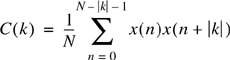
where x(k) represents the kth speech sample. The autocorrelation function is often normalized to the variance of the speech signal and hence is constrained to have values in the range {–1,1} with C(0) = 1. Typical signals have an adjacent sample correlation, C(1), as high as 0.85 to 0.9.
Power Spectral Density function (PSD)—. The nonflat characteristic of the power spectral density of speech makes it possible to obtain significant compression by coding speech in the frequency domain. The nonflat nature of the PSD is basically a frequency domain manifestation of the nonzero autocorrelation property. Typical long-term averaged PSDs of speech show that high frequency components contribute very little to the total speech energy. This indicates that coding speech separately in different frequency bands can lead to significant coding gain. However, it should be noted that the high frequency components, though insignificant in energy are very important carriers of speech information and hence need to be adequately represented in the coding system.
A qualitative measure of the theoretical maximum coding gain that can be obtained by exploiting the nonflat characteristics of the speech spectra is given by the spectral flatness measure (SFM). The SFM is defined as the ratio of the arithmetic to geometric mean of the samples of the PSD taken at uniform intervals in frequency. Mathematically,

where, Sk is the kth frequency sample of the PSD of the speech signal. Typically, speech signals have a long-term SFM value of 8 and a short-time SFM value varying widely between 2 and 500.
Quantization is the process of mapping a continuous range of amplitudes of a signal into a finite set of discrete amplitudes. Quantizers can be thought of as devices that remove the irrelevancies in the signal, and their operation is irreversible. Unlike sampling, quantization introduces distortion. Amplitude quantization is an important step in any speech coding process, and it determines to a great extent the overall distortion as well as the bit rate necessary to represent the speech waveform. A quantizer that uses n bits can have M = 2n discrete amplitude levels. The distortion introduced by any quantization operation is directly proportional to the square of the step size, which in turn is inversely proportional to the number of levels for a given amplitude range. One of the most frequently used measures of distortion is the mean square error distortio which is defined as:
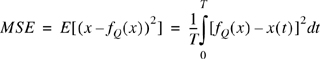
where x(t) represents the original speech signal and fQ(t) represents the quantized speech signal. The distortion introduced by a quantizer is often modeled as additive quantization noise, and the performance of a quantizer is measured as the output signal-to-quantization noise ratio (SQNR). A pulse code modulation (PCM) coder is basically a quantizer of sampled speech amplitudes. PCM coding, using 8 bits per sample at a sampling frequency of 8 kHz, was the first digital coding standard adopted for commercial telephony. The SQNR of a PCM encoder is related to the number of bits used for encoding through the following relation:
where α = 4.77 dB for peak SQNR and α = 0 dB for the average SQNR. The above equation indicates that with every additional bit used for encoding, the output SQNR improves by 6 dB.
The performance of a quantizer can be improved by distributing the quantization levels in a more efficient manner. Nonuniform quantizers distribute the quantization levels in accordance with the pdf of the input waveform. For an input signal with a pdf p(x), the mean square distortion is given by

where fQ(x) is the output of the quantizer. From the above equation, it is clear that the total distortion can be reduced by decreasing the quantization noise, [x-fQ(x)]2, where the pdf, p(x), is large. This means that quantization levels need to be concentrated in amplitude regions of high probability.
To design an optimal nonuniform quantizer, we need to determine the quantization levels which will minimize the distortion of a signal with a given pdf. The Lloyd–Max algorithm [Max60] provides a method to determine the optimum quantization levels by iteratively changing the quantization levels in a manner that minimizes the mean square distortion.
A simple and robust implementation of a nonuniform quantizer used in commercial telephony is the logarithmic quantizer. This quantizer uses fine quantization steps for the frequently occurring low amplitudes in speech and uses much coarser steps for the less frequent, large amplitude excursions. Different companding techniques known as μ-law and A-law companding are used in the US and Europe, respectively.
Nonuniform quantization is obtained by first passing the analog speech signal through a compression (logarithmic) amplifier, and then passing the compressed speech into a standard uniform quantizer. In US μ-law companding, weak speech signals are amplified where strong speech signals are compressed. Let the speech voltage level into the compander be w(t) and the speech output voltage be vo(t). Following [Smi57],
where μ is a positive constant and has a value typically between 50 and 300. The peak value of w(t) is normalized to 1.
In Europe, A-law companding is used [Cat69], and is defined by

Example 8.1.
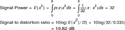
Let the input signal to a quantizer have a probability density function (pdf) as shown in Figure E8.1. Assume the quantization levels to be {1, 3, 5, 7}. Compute the mean square error distortion at the quantizer output and the output signal-to-distortion ratio. How would you change the distribution of quantization levels to decrease the distortion? For what input pdf would this quantizer be optimal?
Solution
From Figure E8.1, the pdf of the input signal can be recognized as:
Given the quantization levels to be {1, 3, 5, 7}, we can define the quantization boundaries as {0, 2, 4, 6, 8}.
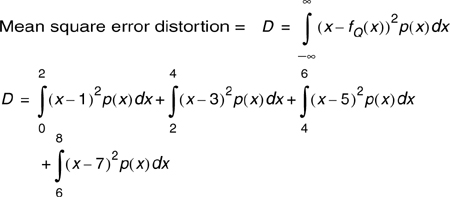
This expression evaluates to 0.333.
To minimize the distortion, we need to concentrate the quantization levels in regions of higher probability. Since the input signal has a greater probability of higher amplitude levels than lower amplitudes, we need to place the quantization levels closer (i.e., more quantization levels) at amplitudes close to eight and farther (i.e., less quantization levels) at amplitudes close to zero.
Since this quantizer has quantization levels uniformly distributed, this would be optimal for an input signal with a uniform pdf.
As noted earlier, there is a distinction between the long term and short term pdf of speech waveforms. This fact is a result of the nonstationarity of speech signals. The time-varying or nonstationary nature of speech signals results in a dynamic range of 40 dB or more. An efficient way to accommodate such a huge dynamic range is to adopt a time varying quantization technique. An adaptive quantizer varies its step size in accordance to the input speech signal power. Its characteristics shrink and expand in time like an accordion. The idea is illustrated in Figure 8.2 through two snapshots of the quantizer characteristics at two different times. The input power level of the speech signal varies slowly enough that simple adaptation algorithms can be easily designed and implemented. One simple adaptation strategy would be to make the step size, Δk, of the quantizer at any given sampling instant, proportional to the quantizer output fQ at the preceding sampling instant as shown below.
Since the adaptation follows the quantizer output rather than the input, step size information need not be explicitly transmitted, but can be recreated at the receiver.
Shannon’s Rate-Distortion Theorem [Sha48] states that there exists a mapping from a source waveform to output code words such that for a given distortion D, R(D) bits per sample are sufficient to reconstruct the waveform with an average distortion arbitrarily close to D. Therefore, the actual rate R has to be greater than R(D). The function R(D), called the rate-distortion function, represents a fundamental limit on the achievable rate for a given distortion. Scalar quantizers do not achieve performance close to this information theoretical limit. Shannon predicted that better performance can be achieved by coding many samples at a time instead of one sample at a time.
Vector quantization (VQ) [Gra84] is a delayed-decision coding technique which maps a group of input samples (typically a speech frame), called a vector, to a code book index. A code book is set up consisting of a finite set of vectors covering the entire anticipated range of values. In each quantizing interval, the code-book is searched and the index of the entry that gives the best match to the input signal frame is selected. Vector quantizers can yield better performance even when the samples are independent of one another. Performance is greatly enhanced if there is strong correlation between samples in the group.
The number of samples in a block (vector) is called the dimension L of the vector quantizer. The rate R of the vector quantizer is defined as:
where n is the size of the VQ code book. R may take fractional values also. All the quantization principles used in scalar quantization apply to vector quantization as a straightforward extension. Instead of quantization levels, we have quantization vectors, and distortion is measured as the squared Euclidean distance between the quantization vector and the input vector.
Vector quantization is known to be most efficient at very low bit rates (R = 0.5 bits/sample or less). This is because when R is small, one can afford to use a large vector dimension L, and yet have a reasonable size, 2RL, of the VQ code book. Use of larger dimensions tends to bring out the inherent capability of VQ to exploit the redundancies in the components of the vector being quantized. Vector quantization is a computationally intensive operation and, for this reason, is not often used to code speech signals directly. However, it is used in many speech coding systems to quantize the speech analysis parameters like the linear prediction coefficients, spectral coefficients, filter bank energies, etc. These systems use improved versions of VQ algorithms which are more computationally efficient such as the multistage VQ, tree-structured VQ, and shape-gain VQ.
Pulse code modulation systems do not attempt to remove the redundancies in the speech signal. Adaptive differential pulse code modulation (ADPCM) [Jay84] is a more efficient coding scheme which exploits the redundancies present in the speech signal. As mentioned earlier, adjacent samples of a speech waveform are often highly correlated. This means that the variance of the difference between adjacent speech amplitudes is much smaller than the variance of the speech signal itself. ADPCM allows speech to be encoded at a bit rate of 32 kbps, which is half the standard 64 kbps PCM rate, while retaining the same voice quality. Efficient algorithms for ADPCM have been developed and standardized. The CCITT standard G.721 ADPCM algorithm for 32 kbps speech coding is used in cordless telephone systems like CT2 and DECT.
In a differential PCM scheme, the encoder quantizes a succession of adjacent sample differences, and the decoder recovers an approximation to the original speech signal by essentially integrating quantized adjacent sample differences. Since the quantization error variance for a given number of bits/sample R, is directly proportional to the input variance, the reduction obtained in the quantizer input variance leads directly to a reduction of reconstruction error variance for a given value of R.
In practice, ADPCM encoders are implemented using signal prediction techniques. Instead of encoding the difference between adjacent samples, a linear predictor is used to predict the current sample. The difference between the predicted and actual sample called the prediction error is then encoded for transmission. Prediction is based on the knowledge of the autocorrelation properties of speech.
Figure 8.3 shows a simplified block diagram of an ADPCM encoder used in the CT2 cordless telephone system [Det89]. This encoder consists of a quantizer that maps the input signal sample onto a four-bit output sample. The ADPCM encoder makes best use of the available dynamic range of four bits by varying its step size in an adaptive manner. The step size of the quantizer depends on the dynamic range of the input, which is speaker dependent and varies with time. The adaptation is, in practice, achieved by normalizing the input signals via a scaling factor derived from a prediction of the dynamic range of the current input. This prediction is obtained from two components: a fast component for signals with rapid amplitude fluctuations and a slow component for signals that vary more slowly. The two components are weighted to give a single quantization scaling factor. It should be noted that the two feedback signals that drive the algorithm—se(k), the estimate of the input signal and y(k), the quantization scaling factor—are ultimately derived solely from I(k), the transmitted 4-bit ADPCM signal. The ADPCM encoder at the transmitter and the ADPCM decoder, at the receiver, are thus driven by the same control signals, with decoding simply the reverse of encoding.
Example 8.2.
In an adaptive PCM system for speech coding, the input speech signal is sampled at 8 kHz, and each sample is represented by 8 bits. The quantizer step size is recomputed every 10 ms, and it is encoded for transmission using 5 bits. Compute the transmission bit rate of such a speech coder. What would be the average and peak SQNR of this system?
Solution
Given:
Sampling frequency = fs = 8 kHz
Number of bits per sample = n = 8 bits
Number of information bits per second = 8000 × 8 = 64000 bits
Since the quantization step size is recomputed every 10 ms, we have 100 step size samples to be transmitted every second.
Therefore, the number of overhead bits = 100 × 5 = 500 bits/s
Therefore, the effective transmission bit rate = 64000 + 500 = 64.5 kbps.
The signal-to-quantization noise ratio depends only on the number of bits used to quantize the samples.
Peak signal to quantization noise ratio in dB = 6.02n + 4.77 = (6.02 × 8) + 4.77 = 52.93 dB.
Average signal-to-noise ratio in dB = 6.02n = 48.16 dB.
Frequency domain coders [Tri79] are a class of speech coders which take advantage of speech perception and generation models without making the algorithm totally dependent on the models used. In this class of coders, the speech signal is divided into a set of frequency components which are quantized and encoded separately. In this way, different frequency bands can be preferentially encoded according to some perceptual criteria for each band, and hence the quantization noise can be contained within bands and prevented from creating harmonic distortions outside the band. These schemes have the advantage that the number of bits used to encode each frequency component can be dynamically varied and shared among the different bands.
Many frequency domain coding algorithms, ranging from simple to complex are available. The most common types of frequency domain coding include sub-band coding (SBC) and block transform coding. While a sub-band coder divides the speech signal into many smaller sub-bands and encodes each sub-band separately according to some perceptual criterion, a transform coder codes the short-time transform of a windowed sequence of samples and encodes them with number of bits proportional to its perceptual significance.
Sub-band coding can be thought of as a method of controlling and distributing quantization noise across the signal spectrum. Quantization is a nonlinear operation which produces distortion products that are typically broad in spectrum. The human ear does not detect the quantization distortion at all frequencies equally well. It is therefore possible to achieve substantial improvement in quality by coding the signal in narrower bands. In a sub-band coder, speech is typically divided into four or eight sub-bands by a bank of filters, and each sub-band is sampled at a bandpass Nyquist rate (which is lower than the original sampling rate) and encoded with different accuracy in accordance to a perceptual criteria. Band-splitting can be done in many ways. One approach could be to divide the entire speech band into unequal sub-bands that contribute equally to the articulation index. One partitioning of the speech band according to this method as suggested by Crochiere et al. [Cro76] is given below.
Sub-band Number | Frequency Range |
|---|---|
1 | 200–700 Hz |
2 | 700–1310 Hz |
3 | 1310–2020 Hz |
4 | 2020–3200 Hz |
Another way to split the speech band would be to divide it into equal width sub-bands and assign to each sub-band number of bits proportional to perceptual significance while encoding them. Instead of partitioning into equal width bands, octave band splitting is often employed. As the human ear has an exponentially decreasing sensitivity to frequency, this kind of splitting is more in tune with the perception process.
There are various methods for processing the sub-band signals. One obvious way is to make a low pass translation of the sub-band signal to zero frequency by a modulation process equivalent to single sideband modulation. This kind of translation facilitates sampling rate reduction and possesses other benefits that accrue from coding low-pass signals. Figure 8.4 shows a simple means of achieving this low pass translation. The input signal is filtered with a bandpass filter of width wn for the n th band. w1n is the lower edge of the band and w2n is the upper edge of the band. The resulting signal sn(t) is modulated by a cosine wave cos (w1nt), and filtered using a low pass filter hn(t) with bandwidth (0 − wn). The resulting signal rn(t) corresponds to the low pass translated version of sn(t) and can be expressed as
where ⊗ denotes a convolution operation. The signal rn(t) is sampled at a rate 2wn. This signal is then digitally encoded and multiplexed with encoded signals from other channels as shown in Figure 8.4. At the receiver, the data is demultiplexed into separate channels, decoded, and bandpass translated to give the estimate of rn(t) for the nth channel.
The low pass translation technique is straightforward and takes advantage of a bank of nonoverlapping bandpass filters. Unfortunately, unless we use sophisticated bandpass filters, this approach will lead to perceptible aliasing effects. Estaban and Galand proposed [Est77] a scheme which avoids this inconvenience even with quasiperfect, sub-band splitting. Filter banks known as quadrature mirror filters (QMFs) are used to achieve this. By designing a set of mirror filters which satisfy certain symmetry conditions, it is possible to obtain perfect alias cancellation. This facilitates the implementation of sub-band coding without the use of very high order filters. This is particularly attractive for real time implementation as a reduced filter order means a reduced computational load and also a reduced latency.
Sub-band coding can be used for coding speech at bit rates in the range 9.6 kbps to 32 kbps. In this range, speech quality is roughly equivalent to that of ADPCM at an equivalent bit rate. In addition, its complexity and relative speech quality at low bit rates make it particularly advantageous for coding below about 16 kbps. However, the increased complexity of sub-band coding when compared to other higher bit rate techniques does not warrant its use at bit rates greater than about 20 kbps. The CD-900 cellular telephone system uses sub-band coding for speech compression.
Example 8.3.
Consider a sub-band coding scheme where the speech bandwidth is partitioned into four bands. The Table below gives the corner frequencies of each band along with the number of bits used to encode each band. Assuming that no side information need be transmitted, compute the minimum encoding rate of this SBC coder.
Sub-band Number | Frequency Band (Hz) | # of Encoding Bits |
|---|---|---|
1 | 225–450 | 4 |
2 | 450–900 | 3 |
3 | 1000–1500 | 2 |
4 | 1800–2700 | 1 |
Solution
Given:
Number of sub-bands = N = 4
For perfect reconstruction of the band-pass signals, they need to be sampled at a Nyquist rate equal to twice the bandwidth of the signal.
Therefore, the different sub-bands need to be sampled at the following rates:
Sub-band 1 = 2 × (450 – 225) = 450 samples/s
Sub-band 2 = 2 × (900 – 450) = 900 samples/s
Sub-band 3 = 2 × (1500 – 1000) = 1000 samples/s
Sub-band 4 = 2 × (2700 – 1800) = 1800 samples/s
Now, total encoding rate is
450 × 4 + 900 × 3 + 1000 × 2 + 1800 × 1 = 8300 bits/s = 8.3 kbps
Adaptive transform coding (ATC) [Owe93] is another frequency domain technique that has been successfully used to encode speech at bit rates in the range 9.6 kbps to 20 kbps. This is a more complex technique which involves block transformations of windowed input segments of the speech waveform. Each segment is represented by a set of transform coefficients, which are separately quantized and transmitted. At the receiver, the quantized coefficients are inverse transformed to produce a replica of the original input segment.
One of the most attractive and frequently used transforms for speech coding is the discrete cosine transform (DCT). The DCT of a N-point sequence x(n) is defined as
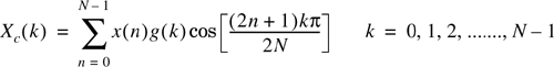
where g(0) = 1 and ![]() , k = 1,2, ......., N − 1. The inverse DCT is defined as:
, k = 1,2, ......., N − 1. The inverse DCT is defined as:

In practical situations the DCT and IDCT are not evaluated directly using the above equations. Fast algorithms developed for computing the DCT in a computationally efficient manner are used.
Most of the practical transform coding schemes vary the bit allocation among different coefficients adaptively from frame to frame while keeping the total number of bits constant. This dynamic bit allocation is controlled by time-varying statistics which have to be transmitted as side information. This constitutes an overhead of about 2 kbps. The frame of N samples to be transformed or inverse-transformed is accumulated in the buffer in the transmitter and receiver respectively. The side information is also used to determine the step size of the various coefficient quantizers. In a practical system, the side information transmitted is a coarse representation of the log-energy spectrum. This typically consists of L frequency points, where L is in the range 15–20, which are computed by averaging sets of N/L adjacent squared values of the transform coefficients X(k). At the receiver, an N-point spectrum is reconstructed from the L-point spectrum by geometric interpolation in the log-domain. The number of bits assigned to each transform coefficient is proportional to its corresponding spectral energy value.
Vocoders are a class of speech coding systems that analyze the voice signal at the transmitter, transmit parameters derived from the analysis, and then synthesize the voice at the receiver using those parameters. All vocoder systems attempt to model the speech generation process as a dynamic system and try to quantify certain physical constraints of the system. These physical constraints are used to provide a parsimonious description of the speech signal. Vocoders are, in general, much more complex than the waveform coders and achieve very high economy in transmission bit rate. However, they are less robust, and their performance tends to be talker dependent. The most popular among the vocoding systems is the linear predictive coder (LPC). The other vocoding schemes include the channel vocoder, formant vocoder, cepstrum vocoder and voice excited vocoder.
Figure 8.5 shows the traditional speech generation model that is the basis of all vocoding systems [Fla79]. The sound generating mechanism forms the source and is linearly separated from the intelligence modulating vocal tract filter which forms the system. The speech signal is assumed to be of two types: voiced and unvoiced. Voiced sound (“m”, “n”, “v” pronunciations) are a result of quasiperiodic vibrations of the vocal chord and unvoiced sounds (“f”, “s”, “sh” pronunciations) are fricatives produced by turbulent air flow through a constriction. The parameters associated with this model are the voice pitch, the pole frequencies of the modulating filter, and the corresponding amplitude parameters. The pitch frequency for most speakers is below 300 Hz, and extracting this information from the signal is very difficult. The pole frequencies correspond to the resonant frequencies of the vocal tract and are often called the formants of the speech signal. For adult speakers, the formants are centered around 500 Hz, 1500 Hz, 2500 Hz, and 3500 Hz. By meticulously adjusting the parameters of the speech generation model, good quality speech can be synthesized.
The channel vocoder was the first among the analysis–synthesis systems of speech demonstrated practically. Channel vocoders are frequency domain vocoders that determine the envelope of the speech signal for a number of frequency bands and then sample, encode, and multiplex these samples with the encoded outputs of the other filters. The sampling is done synchronously every 10 ms to 30 ms. Along with the energy information about each band, the voiced/unvoiced decision, and the pitch frequency for voiced speech are also transmitted.
The formant vocoder [Bay73] is similar in concept to the channel vocoder. Theoretically, the formant vocoder can operate at lower bit rates than the channel vocoder because it uses fewer control signals. Instead of sending samples of the power spectrum envelope, the formant vocoder attempts to transmit the positions of the peaks (formants) of the spectral envelope. Typically, a formant vocoder must be able to identify at least three formants for representing the speech sounds, and it must also control the intensities of the formants.
Formant vocoders can reproduce speech at bit rates lower than 1200 bits/s. However, due to difficulties in accurately computing the location of formants and formant transitions from human speech, they have not been very successful.
The Cepstrum vocoder separates the excitation and vocal tract spectrum by inverse Fourier transforming of the log magnitude spectrum to produce the cepstrum of the signal. The low frequency coefficients in the cepstrum correspond to the vocal tract spectral envelope, with the high frequency excitation coefficients forming a periodic pulse train at multiples of the sampling period. Linear filtering is performed to separate the vocal tract cepstral coefficients from the excitation coefficients. In the receiver, the vocal tract cepstral coefficients are Fourier transformed to produce the vocal tract impulse response. By convolving this impulse response with a synthetic excitation signal (random noise or periodic pulse train), the original speech is reconstructed.
Voice-excited vocoders eliminate the need for pitch extraction and voicing detection operations. This system uses a hybrid combination of PCM transmission for the low frequency band of speech, combined with channel vocoding of higher frequency bands. A pitch signal is generated at the synthesizer by rectifying, bandpass filtering, and clipping the baseband signal, thus creating a spectrally flat signal with energy at pitch harmonics. Voice excited vocoders have been designed for operation at 7200 bits/s to 9600 bits/s, and their quality is typically superior to that obtained by the traditional pitch excited vocoders.
Linear predictive coders (LPCs) [Sch85a] belong to the time domain class of vocoders. This class of vocoders attempts to extract the significant features of speech from the time waveform. Though LPC coders are computationally intensive, they are by far the most popular among the class of low bit rate vocoders. With LPC, it is possible to transmit good quality voice at 4.8 kbps and poorer quality voice at even lower rates.
The linear predictive coding system models the vocal tract as an all pole linear filter with a transfer function described by
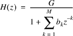
where G is a gain of the filter and z-1 represents a unit delay operation. The excitation to this filter is either a pulse at the pitch frequency or random white noise depending on whether the speech segment is voiced or unvoiced. The coefficients of the all pole filter are obtained in the time domain using linear prediction techniques [Mak75]. The prediction principles used are similar to those in ADPCM coders. However, instead of transmitting quantized values of the error signal representing the difference between the predicted and actual waveform, the LPC system transmits only selected characteristics of the error signal. The parameters include the gain factor, pitch information, and the voiced/unvoiced decision information, which allow approximation of the correct error signal. At the receiver, the received information about the error signal is used to determine the appropriate excitation for the synthesis filter. That is, the error signal is the excitation to the decoder. The synthesis filter is designed at the receiver using the received predictor coefficients. In practice, many LPC coders transmit the filter coefficients which already represent the error signal and can be directly synthesized by the receiver. Figure 8.6 shows a block diagram of an LPC system [Jay86].
Determination of Predictor Coefficients—. The linear predictive coder uses a weighted sum of p past samples to estimate the present sample, where p is typically in the range of 10–15. Using this technique, the current sample sn can be written as a linear sum of the immediately preceding samples sn-k
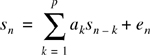
where en is the prediction error (residual). The predictor coefficients are calculated to minimize the average energy E in the error signal that represents the difference between the predicted and actual speech amplitude
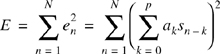
where a0 = −1. Typically, the error is computed for a time window of 10 ms, which corresponds to a value of N = 80. To minimize E with respect to am, it is required to set the partial derivatives equal to zero

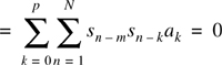
The inner summation can be recognized as the correlation coefficient Crm and hence the above equation can be rewritten as
After determining the correlation coefficients Crm, Equation (8.18) can be used to determine the predictor coefficients. Equation (8.18) is often expressed in matrix notation and the predictor coefficients calculated using matrix inversion. A number of algorithms have been developed to speed up the calculation of predictor coefficients. Normally, the predictor coefficients are not coded directly, as they would require 8 bits to 10 bits per coefficient for accurate representation [Del93]. The accuracy requirements are lessened by transmitting the reflection coefficients (a closely related parameter), which have a smaller dynamic range. These reflection coefficients can be adequately represented by 6 bits per coefficient. Thus, for a 10th order predictor, the total number of bits assigned to the model parameters per frame is 72, which includes 5 bits for a gain parameter and 6 bits for the pitch period. If the parameters are estimated every 15 ms to 30 ms, the resulting bit rate is in the range of 2400 bps to 4800 bps. The coding of the reflection coefficient can be further improved by performing a nonlinear transformation of the coefficients prior to coding. This nonlinear transformation reduces the sensitivity of the reflection coefficients to quantization errors. This is normally done through a log-area ratio (LAR) transform which performs an inverse hyperbolic tangent mapping of the reflection coefficients, Rn(k)
Various LPC schemes differ in the way they recreate the error signal (excitation) at the receiver. Three alternatives are shown in Figure 8.7 [Luc89]. The first one shows the most popular means. It uses two sources at the receiver, one of white noise and the other with a series of pulses at the current pitch rate. The selection of either of these excitation methods is based on the voiced/unvoiced decision made at the transmitter and communicated to the receiver along with the other information. This technique requires that the transmitter extract pitch frequency information which is often very difficult. Moreover, the phase coherence between the harmonic components of the excitation pulse tends to produce a buzzy twang in the synthesized speech. These problems are mitigated in the other two approaches: Multipulse excited LPC and stochastic or code excited LPC.
Atal showed [Ata86] that, no matter how well the pulse is positioned, excitation by a single pulse per pitch period produces audible distortion. Therefore, he suggested using more than one pulse, typically eight per period, and adjusting the individual pulse positions and amplitudes sequentially to minimize a spectrally weighted mean square error. This technique is called the multipulse excited LPC (MPE-LPC) and results in better speech quality, not only because the prediction residual is better approximated by several pulses per pitch period, but also because the multipulse algorithm does not require pitch detection. The number of pulses used can be reduced, in particular for high pitched voices, by incorporating a linear filter with a pitch loop in the synthesizer.
In this method, the coder and decoder have a predetermined code book of stochastic (zero-mean white Gaussian) excitation signals [Sch85b]. For each speech signal, the transmitter searches through its code book of stochastic signals for the one that gives the best perceptual match to the sound when used as an excitation to the LPC filter. The index of the code book where the best match was found is then transmitted. The receiver uses this index to pick the correct excitation signal for its synthesizer filter. The code excited LPC (CELP) coders are extremely complex and can require more than 500 million multiply and add operations per second. They can provide high quality even when the excitation is coded at only 0.25 bits per sample. These coders can achieve transmission bit rates as low as 4.8 kbps.
Figure 8.8 illustrates the procedure for selecting the optimum excitation signal. The procedure is best illustrated through an example. Consider the coding of a short 5 ms block of speech signal. At a sampling frequency of 8 kHz, each block consists of 40 speech samples. A bit rate of 1/4 bit per sample corresponds to 10 bits per block. Therefore, there are 210 = 1024 possible sequences of length 40 for each block. Each member of the code book provides 40 samples of the excitation signal with a scaling factor that is changed every 5 ms block. The scaled samples are passed sequentially through two recursive filters, which introduce voice periodicity and adjust the spectral envelope. The regenerated speech samples at the output of the second filter are compared with samples of the original speech signal to form a difference signal. The difference signal represents the objective error in the regenerated speech signal. This is further processed through a linear filter which amplifies the perceptually more important frequencies and attenuates the perceptually less important frequencies.
Though computationally intensive, advances in DSP and VLSI technology have made real-time implementation of CELP codecs possible. The CDMA digital cellular standard (IS-95) proposed by QUALCOMM uses a variable rate CELP codec at 1.2 to 14.4 kbps. In 1995, QUALCOMM introduced QCELP13, a 13.4 kbps CELP coder that operates on a 14.4 kbps channel.
The rationale behind the residual excited LPC (RELP) is related to that of the DPCM technique in waveform coding [Del93]. In this class of LPC coders, after estimating the model parameters (LP coefficients or related parameters) and excitation parameters (voiced/unvoiced decision, pitch, gain) from a speech frame, the speech is synthesized at the transmitter and subtracted from the original speech signal to from a residual signal. The residual signal is quantized, coded, and transmitted to the receiver along with the LPC model parameters. At the receiver, the residual error signal is added to the signal generated using the model parameters to synthesize an approximation of the original speech signal. The quality of the synthesized speech is improved due to the addition of the residual error. Figure 8.9 shows a block diagram of a simple RELP codec.
Choosing the right speech codec is an important step in the design of a digital mobile communication system [Gow93]. Because of the limited bandwidth that is available, it is required to compress speech to maximize the number of users on the system. A balance must be struck between the perceived quality of the speech resulting from this compression and the overall system cost and capacity. Other criterion that must be considered include the end-to-end encoding delay, the algorithmic complexity of the coder, the dc power requirements, compatibility with existing standards, and the robustness of the encoded speech to transmission errors.
As seen in Chapter 4 and 5, the mobile radio channel is a hostile transmission medium beset with problems such as fading, multipath, and interference. It is therefore important that the speech codec be robust to transmission errors. Depending on the technique used, different speech coders show varying degree of immunity to transmission errors. For example, under same bit error rate conditions, 40 kbps adaptive delta modulation (ADM) sounds much better than 56 kbps log-PCM [Ste93]. This does not mean that decreasing bit rate enhances the coder robustness to transmission errors. On the contrary, as speech signals are represented by fewer and fewer bits, the information content per bit increases and hence need to be more safely preserved. Low bit rate vocoder type codecs, which do parametric modeling of the vocal tract and auditory mechanisms, have some bits carrying critical information which if corrupted would lead to unacceptable distortion. While transmitting low bit rate encoded speech, it is imperative to determine the perceptual importance of each bit and group them according to their sensitivity to errors. Depending on their perceptual significance, bits in each group are provided with different levels of error protection through the use of different forward error correction (FEC) codes.
The choice of the speech coder will also depend on the cell size used. When the cell size is sufficiently small such that high spectral efficiency is achieved through frequency reuse, it may be sufficient to use a simple high rate speech codec. In the cordless telephone systems like CT2 and DECT, which use very small cells (microcells), 32 kbps ADPCM coders are used to achieve acceptable performance even without channel coding and equalization. Cellular systems operating with much larger cells and poorer channel conditions need to use error correction coding, thereby requiring the speech codecs to operate at lower bit rates. In mobile satellite communications, the cell sizes are very large and the available bandwidth is very small. In order to accommodate realistic number of users the speech rate must be of the order of 3 kbps, requiring the use of vocoder techniques [Ste93].
The type of multiple access technique used, being an important factor in determining the spectral efficiency of the system, strongly influences the choice of speech codec. The US digital TDMA cellular system (IS-136) increased the capacity of the existing analog system (AMPS) threefold by using an 8 kbps VSELP speech codec. CDMA systems, due to their innate interference rejection capabilities and broader bandwidth availability, allow the use of a low bit rate speech codec without regard to its robustness to transmission errors. Transmission errors can be corrected with powerful FEC codes, the use of which, in CDMA systems, does not effect bandwidth efficiency very significantly.
The type of modulation employed also has considerable impact on the choice of speech codec. For example, using bandwidth-efficient modulation schemes can lower the bit rate reduction requirements on the speech codec, and vice versa. Table 8.1 shows a listing of the types of speech codecs used in various digital mobile communication systems.
Table 8.1. Speech Coders Used in Various First and Second Generation Wireless Systems
Standard | Service Type | Speech Coder Type Used | Bit Rate (kbps) |
|---|---|---|---|
GSM | Cellular | RPE-LTP | 9.6, 13 |
CD-900 | Cellular | SBC | 16 |
USDC (IS-136) | Cellular | VSELP | 8 |
IS-95 | Cellular | CELP | 1.2, 2.4, 4.8, 9.6, 13.4, 14.4 |
IS-95 PCS | PCS | CELP | 13.4, 14.4 |
PDC | Cellular | VSELP | 4.5, 6.7, 11.2 |
CT2 | Cordless | ADPCM | 32 |
DECT | Cordless | ADPCM | 32 |
PHS | Cordless | ADPCM | 32 |
DCS-1800 | PCS | RPE-LTP | 13 |
PACS | PCS | ADPCM | 32 |
Example 8.4.
A digital mobile communication system has a forward channel frequency band ranging between 810 MHz to 826 MHz and a reverse channel band between 940 MHz to 956 MHz. Assume that 90 percent of the bandwidth is used by traffic channels. It is required to support at least 1150 simultaneous calls using FDMA. The modulation scheme employed has a spectral efficiency of 1.68 bps/Hz. Assuming that the channel impairments necessitate the use of rate 1/2 FEC codes, find the upper bound on the transmission bit rate that a speech coder used in this system should provide?
Solution
Total Bandwidth available for traffic channels = 0.9 × (810 – 826) = 14.4 MHz.
Number of simultaneous users = 1150.
Therefore, maximum channel bandwidth = 14.4 /1150 MHz = 12.5 kHz.
Spectral Efficiency = 1.68 bps/Hz.
Therefore, maximum channel data rate = 1.68 × 12500 bps = 21 kbps.
FEC coder rate = 0.5.
Therefore, maximum net data rate = 21 × 0.5 kbps = 10.5 kbps.
Therefore, we need to design a speech coder with a data rate less than or equal to 10.5 kbps.
Example 8.5.
The output of a speech coder has bits which contribute to signal quality with varying degree of importance. Encoding is done on blocks of samples of 20 ms duration (260 bits of coder output). The first 50 of the encoded speech bits (say type 1) in each block are considered to be the most significant and hence to protect them from channel errors are appended with 10 CRC bits and convolutionally encoded with a rate 1/2 FEC coder. The next 132 bits (say type 2) are appended with 5 CRC bits and the last 78 bits (say type 3) are not error protected. Compute the gross channel data rate achievable.
Solution
Number of type 1 channel bits to be transmitted every 20 ms (50 + 10) × 2 = 120 bits
Number of type 2 channel bits to be transmitted every 20 ms 132 + 5 = 137 bits
Number of type 3 channel bits to be encoded = 78 bits
Total number of channel bits to be transmitted every 20 ms 120 + 137 + 78 bits = 335 bits
Therefore, gross channel bit rate = 335/(20 × 10−3) = 16.75 kbps.
The original speech coder used in the pan-European digital cellular standard GSM goes by a rather grandiose name of regular pulse excited long-term prediction (RPE-LTP) codec. This codec has a net bit rate of 13 kbps and was chosen after conducting exhaustive subjective tests [Col89] on various competing codecs. More recent GSM upgrades have improved upon the original codec specification.
The RPE-LTP codec [Var88] combines the advantages of the earlier French proposed baseband RELP codec with those of the multipulse excited long-term prediction (MPE-LTP) codec proposed by Germany. The advantage of the baseband RELP codec is that it provides good quality speech at low complexity. The speech quality of a RELP codec is, however, limited due to the tonal noise introduced by the process of high frequency regeneration and by the bit errors introduced during transmission. The MPE-LTP technique, on the other hand, produces excellent speech quality at high complexity and is not much affected by bit errors in the channel. By modifying the RELP codec to incorporate certain features of the MPE-LTP codec, the net bit rate was reduced from 14.77 kbps to 13.0 kbps without loss of quality. The most important modification was the addition of a long-term prediction loop.
The GSM codec is relatively complex and power hungry. Figure 8.10 shows a block diagram of the speech encoder [Ste94]. The encoder is comprised of four major processing blocks. The speech sequence is first pre-emphasized, ordered into segments of 20 ms duration, and then Hamming-windowed. This is followed by short-term prediction (STP) filtering analysis where the logarithmic area ratios (LARs) of the reflection coefficients rn(k) (eight in number) are computed. The eight LAR parameters have different dynamic ranges and probability distribution functions, and hence all of them are not encoded with the same number of bits for transmission. The LAR parameters are also decoded by the LPC inverse filter so as to minimize the error en.
LTP analysis which involves finding the pitch period pn and gain factor gn is then carried out such that the LTP residual rn is minimized. To minimize rn, pitch extraction is done by the LTP by determining that value of delay, D, which maximizes the cross-correlation between the current STP error sample, en, and a previous error sample en-D. The extracted pitch pn and gain gn are transmitted and encoded at a rate of 3.6 kbps. The LTP residual, rn, is weighted and decomposed into three candidate excitation sequences. The energies of these sequences are identified, and the one with the highest energy is selected to represent the LTP residual. The pulses in the excitation sequence are normalized to the highest amplitude, quantized, and transmitted at a rate of 9.6 kbps.
Figure 8.11 shows a block diagram of the GSM speech decoder [Ste94]. It consists of four blocks which perform operations complementary to those of the encoder. The received excitation parameters are RPE decoded and passed to the LTP synthesis filter which uses the pitch and gain parameter to synthesize the long-term signal. Short-term synthesis is carried out using the received reflection coefficients to recreate the original speech signal.
Every 260 bits of the coder output (i.e., 20 ms blocks of speech) are ordered, depending on their importance, into groups of 50, 132, and 78 bits each. The bits in the first group are very important bits called type Ia bits. The next 132 bits are important bits called Ib bits, and the last 78 bits are called type II bits. Since type Ia bits are the ones which effect speech quality the most, they have error detection CRC bits added. Both Ia and Ib bits are convolutionally encoded for forward error correction. The least significant type II bits have no error correction or detection.
The US digital cellular system (IS-136) uses a vector sum excited linear predictive coder (VSELP). This coder operates at a raw data rate of 7950 bits/s and a total data rate of 13 kbps after channel coding. The VSELP coder was developed by a consortium of companies, and the Motorola implementation was selected as the speech coding standard after extensive testing.
The VSELP speech coder is a variant of the CELP type vocoders [Ger90]. This coder was designed to accomplish the three goals of highest speech quality, modest computational complexity, and robustness to channel errors. The code books in the VSELP encoder are organized with a predefined structure such that a brute-force search is avoided. This significantly reduces the time required for the optimum code word search. These code books also impart high speech quality and increased robustness to channel errors while maintaining modest complexity.
Figure 8.12 shows a block diagram of a VSELP encoder. The 8 kbps VSELP codec utilizes three excitation sources. One is from the long-term (“pitch”) predictor state, or adaptive code book. The second and third sources are from the two VSELP excitation code books. Each of these VSELP code books contain the equivalent of 128 vectors. These three excitation sequences are multiplied by their corresponding gain terms and summed to give the combined excitation sequence. After each subframe, the combined excitation sequence is used to update the long-term filter state (adaptive code book). The synthesis filter is a direct form 10th order LPC all pole-filter. The LPC coefficients are coded once per 20 ms frame and updated in each 5 ms subframe. The number of samples in a subframe is 40 at an 8 kHz sampling rate. The decoder is shown in Figure 8.13.
There are two approaches to evaluating the performance of a speech coder in terms of its ability to preserve the signal quality [Jay84]. Objective measures have the general nature of a signal-to-noise ratio and provide a quantitative value of how well the reconstructed speech approximates the original speech. Mean square error (MSE) distortion, frequency weighted MSE, and segmented SNR, articulation index are examples of objective measures. While objective measures are useful in initial design and simulation of coding systems, they do not necessarily give an indication of speech quality as perceived by the human ear. Since the listener is the ultimate judge of the signal quality, subjective listening tests constitute an integral part of speech coder evaluation.
Subjective listening tests are conducted by playing the sample to a number of listeners and asking them to judge the quality of the speech. Speech coders are highly speaker dependent in that the quality varies with the age and gender of the speaker, the speed at which the speaker speaks, and other factors. The subjective tests are carried out in different environments to simulate real life conditions such as noisy, multiple speakers, etc. These tests provide results in terms of overall quality, listening effort, intelligibility, and naturalness. The intelligibility tests measure the listeners ability to identify the spoken word. The diagnostic rhyme test (DRT) is the most popular and widely used intelligibility test. In this test, a word from a pair of rhymed words such as “those-dose” is presented to the listener and the listener is asked to identify which word was spoken. Typical percentage correct on the DRT tests range from 75–90. The diagnostic acceptability measure (DAM) is another test that evaluates acceptability of speech coding systems. All these tests results are difficult to rank and hence require a reference system. The most popular ranking system is known as the mean opinion score or MOS ranking. This is a five point quality ranking scale with each point associated with a standardized descriptions: bad, poor, fair, good, excellent. Table 8.2 gives a listing of the mean square opinion ranking system.
Table 8.2. MOS Quality Rating [Col89]
Quality Scale | Score | Listening Effort Scale |
|---|---|---|
Excellent | 5 | No effort required |
Good | 4 | No appreciable effort required |
Fair | 3 | Moderate effort required |
Poor | 2 | Considerable effort required |
Bad | 1 | No meaning understood with reasonable effort |
One of the most difficult conditions for speech coders to perform well in is the case where a digital speech-coded signal is transmitted from the mobile to the base station, and then demodulated into an analog signal which is then speech coded for retransmission as a digital signal over a landline or wireless link. This situation, called tandem signaling, tends to exaggerate the bit errors originally received at the base station. Tandem signaling is difficult to protect against, but is an important evaluation criterion in the evaluation of speech coders. As wireless systems proliferate, there will be a greater demand for mobile-to-mobile communications, and such links will, by definition, involve at least two independent, noisy tandems.
In general, the MOS rating of a speech codec decreases with decreasing bit rate. Table 8.3 gives the performance of some of the popular speech coders on the MOS scale.
8.1 | For an 8 bit uniform quantizer that spans the range (–1 V, 1 V), determine the step size of the quantizer. Compute the SNR due to quantization if the signal is a sinusoid that spans the entire range of the quantizer. |
8.2 | Derive a general expression that relates the signal-to-noise ratio due to quantization as a function of the number of bits. |
8.3 | For a μ-law compander with μ = 255, plot the magnitude of the output voltage as a function of the magnitude of the input voltage. If an input voltage of 0.1 V is applied to the compander, what is the resulting output voltage? If an input voltage of 0.01 V is applied to the input, determine the resulting output voltage. Assume the compander has a maximum input of 1 V. |
8.4 | For an A-law compander with A = 90, plot the magnitude of the output voltage as a function of the magnitude of the input voltage. If an input voltage of 0.1 V is applied to the compander, what is the resulting output voltage? If an input voltage of 0.01 V is applied to the input, determine the resulting output voltage. Assume the compander has a maximum input of 1 V. |
8.5 | A compander relies on speech compression and speech expansion (decompression) at the receiver in order to restore signals to their correct relative values. The expander has an inverse characteristic when compared to the compressor. Determine the proper compressor characteristics for the speech compressors in Problems 8.3 and 8.4. |
8.6 | A speech signal has an amplitude pdf that can be characterized as a zero-mean Gaussian process with a standard deviation of 0.5 V. For such a speech signal, determine the mean square error distortion at the output of a 4 bit quantizer if quantization levels are uniformly spaced by 0.25 V. Design a nonuniform quantizer that would minimize the mean square error distortion, and determine the level of distortion. |
8.7 | Consider a sub-band speech coder that allocates 5 bits for the audio spectrum between 225 Hz and 500 Hz, 3 bits for 500 Hz to 1200 Hz, and 2 bits for frequencies between 1300 Hz and 3 kHz. Assume that the sub-band coder output is then applied to a rate 3/4 convolutional coder. Determine the data rate out of the channel coder. |
8.8 | List four significant factors which influence the choice of speech coders in mobile communication systems. Elaborate on the tradeoffs which are caused by each factor. Rank order the factors based on your personal view point, and defend your position. |
8.9 | Professors Deller, Proakis, and Hansen co-authored an extensive text entitled “Discrete-Time Processing of Speech Signals” [Del93]. As part of this work, they have created an Internet “ftp” site which contains numerous speech files. Browse the site and download several files which demonstrate several speech coders. Report your findings and indicate which files you found to be most useful. The files are available via ftp at archive.egr.msu.edu in the directory pub/jojo/DPHTEXT. The file README.DPH includes instructions and file descriptions. These files are in ASCII, one signed integer decimal sample per line, and are easily read by MATLAB. |
8.10 | Scalar quantization computer program: Consider a data sequence of random variables {Xi}, where each Xi~N(0,1) has a Gaussian distribution with mean zero and variance 1. Construct a scalar quantizer which quantizes each sample at a rate of 3 bits/sample (so there will be eight quantizer levels). Use the generalized Lloyd algorithm to determine your quantization levels. Train your quantizer on a sequence of 250 samples. Your solution should include:
|
8.11 | Vector quantization computer program: Consider data sequence of random variables {Xi}, where each Xi~N(0,1) has a Gaussian distribution with mean zero and variance 1. Now construct a two-dimensional vector quantizer which quantizes each sample at a rate of 3 bits/sample (so there will be 8 × 8 = 64 quantization vectors). Use the generalized Lloyd algorithm to determine your quantization vectors. Train your quantizer using a sequence of 1200 vectors (2400 samples). Your solution should include:
|
8.12 | Vector quantization with correlated samples: Consider a sequence of random variables {Yi} and {Xi}, where Xi~N(0,1), Y1~N(0,1) and As a result, each Yi in the sequence {Yi} will have a Gaussian distribution with mean zero and variance 1, but the samples will be correlated (this is a simple example of what is called a Gauss–Markov Source). Now construct a two-dimensional vector quantizer which quantizes each sample at a rate of 3 bits/sample. Use the generalized Lloyd algorithm to determine your quantization vectors. Train your quantizer on a sequence of 1200 vectors (2400 samples). Your solution should include:
|