Small-scale fading, or simply fading, is used to describe the rapid fluctuations of the amplitudes, phases, or multipath delays of a radio signal over a short period of time or travel distance, so that large-scale path loss effects may be ignored. Fading is caused by interference between two or more versions of the transmitted signal which arrive at the receiver at slightly different times. These waves, called multipath waves, combine at the receiver antenna to give a resultant signal which can vary widely in amplitude and phase, depending on the distribution of the intensity and relative propagation time of the waves and the bandwidth of the transmitted signal.
Multipath in the radio channel creates small-scale fading effects. The three most important effects are:
Rapid changes in signal strength over a small travel distance or time interval
Random frequency modulation due to varying Doppler shifts on different multipath signals
Time dispersion (echoes) caused by multipath propagation delays.
In built-up urban areas, fading occurs because the height of the mobile antennas are well below the height of surrounding structures, so there is no single line-of-sight path to the base station. Even when a line-of-sight exists, multipath still occurs due to reflections from the ground and surrounding structures. The incoming radio waves arrive from different directions with different propagation delays. The signal received by the mobile at any point in space may consist of a large number of plane waves having randomly distributed amplitudes, phases, and angles of arrival. These multipath components combine vectorially at the receiver antenna, and can cause the signal received by the mobile to distort or fade. Even when a mobile receiver is stationary, the received signal may fade due to movement of surrounding objects in the radio channel.
If objects in the radio channel are static, and motion is considered to be only due to that of the mobile, then fading is purely a spatial phenomenon. The spatial variations of the resulting signal are seen as temporal variations by the receiver as it moves through the multipath field. Due to the constructive and destructive effects of multipath waves summing at various points in space, a receiver moving at high speed can pass through several fades in a small period of time. In a more serious case, a receiver may stop at a particular location at which the received signal is in a deep fade. Maintaining good communications can then become very difficult, although passing vehicles or people walking in the vicinity of the mobile can often disturb the field pattern, thereby diminishing the likelihood of the received signal remaining in a deep null for a long period of time. Antenna space diversity can prevent deep fading nulls, as shown in Chapter 6. Figure 3.1 shows typical rapid variations in the received signal level due to small-scale fading as a receiver is moved over a distance of a few meters.
Due to the relative motion between the mobile and the base station, each multipath wave experiences an apparent shift in frequency. The shift in received signal frequency due to motion is called the Doppler shift, and is directly proportional to the velocity and direction of motion of the mobile with respect to the direction of arrival of the received multipath wave.
Many physical factors in the radio propagation channel influence small-scale fading. These include the following:
Multipath propagation—. The presence of reflecting objects and scatterers in the channel creates a constantly changing environment that dissipates the signal energy in amplitude, phase, and time. These effects result in multiple versions of the transmitted signal that arrive at the receiving antenna, displaced with respect to one another in time and spatial orientation. The random phase and amplitudes of the different multipath components cause fluctuations in signal strength, thereby inducing small-scale fading, signal distortion, or both. Multipath propagation often lengthens the time required for the baseband portion of the signal to reach the receiver which can cause signal smearing due to intersymbol interference.
Speed of the mobile—. The relative motion between the base station and the mobile results in random frequency modulation due to different Doppler shifts on each of the multipath components. Doppler shift will be positive or negative depending on whether the mobile receiver is moving toward or away from the base station.
Speed of surrounding objects—. If objects in the radio channel are in motion, they induce a time varying Doppler shift on multipath components. If the surrounding objects move at a greater rate than the mobile, then this effect dominates the small-scale fading. Otherwise, motion of surrounding objects may be ignored, and only the speed of the mobile need be considered. The coherence time defines the “staticness” of the channel, and is directly impacted by the Doppler shift.
The transmission bandwidth of the signal—. If the transmitted radio signal bandwidth is greater than the “bandwidth” of the multipath channel, the received signal will be distorted, but the received signal strength will not fade much over a local area (i.e., the small-scale signal fading will not be significant). As will be shown, the bandwidth of the channel can be quantified by the coherence bandwidth which is related to the specific multipath structure of the channel. The coherence bandwidth is a measure of the maximum frequency difference for which signals are still strongly correlated in amplitude. If the transmitted signal has a narrow bandwidth as compared to the channel, the amplitude of the signal will change rapidly, but the signal will not be distorted in time. Thus, the statistics of small-scale signal strength and the likelihood of signal smearing appearing over small-scale distances are very much related to the specific amplitudes and delays of the multipath channel, as well as the bandwidth of the transmitted signal.
Consider a mobile moving at a constant velocity v, along a path segment having length d between points X and Y, while it receives signals from a remote source S, as illustrated in Figure 5.1. The difference in path lengths traveled by the wave from source S to the mobile at points X and Y is Δl = d cos θ = vΔt cos θ, where Δt is the time required for the mobile to travel from X to Y, and θ is assumed to be the same at points X and Y since the source is assumed to be very far away. The phase change in the received signal due to the difference in path lengths is therefore
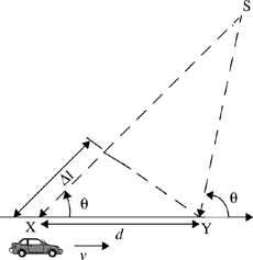
and hence the apparent change in frequency, or Doppler shift, is given by fd, where
Equation (5.2) relates the Doppler shift to the mobile velocity and the spatial angle between the direction of motion of the mobile and the direction of arrival of the wave. It can be seen from Equation (5.2) that if the mobile is moving toward the direction of arrival of the wave, the Doppler shift is positive (i.e., the apparent received frequency is increased), and if the mobile is moving away from the direction of arrival of the wave, the Doppler shift is negative (i.e., the apparent received frequency is decreased). As shown in Section 5.7.1, multipath components from a CW signal that arrive from different directions contribute to Doppler spreading of the received signal, thus increasing the signal bandwidth.
Example 5.1.
Consider a transmitter which radiates a sinusoidal carrier frequency of 1850 MHz. For a vehicle moving 60 mph, compute the received carrier frequency if the mobile is moving (a) directly toward the transmitter, (b) directly away from the transmitter, and (c) in a direction which is perpendicular to the direction of arrival of the transmitted signal.
Solution
Given:
|
|
|
The vehicle is moving directly toward the transmitter.
The Doppler shift in this case is positive and the received frequency is given by Equation (5.2)
The vehicle is moving directly away from the transmitter.
The Doppler shift in this case is negative and hence the received frequency is given by
The vehicle is moving perpendicular to the angle of arrival of the transmitted signal.
In this case, θ = 90°, cosθ = 0, and there is no Doppler shift.
The received signal frequency is the same as the transmitted frequency of 1850 MHz.
The small-scale variations of a mobile radio signal can be directly related to the impulse response of the mobile radio channel. The impulse response is a wideband channel characterization and contains all information necessary to simulate or analyze any type of radio transmission through the channel. This stems from the fact that a mobile radio channel may be modeled as a linear filter with a time varying impulse response, where the time variation is due to receiver motion in space. The filtering nature of the channel is caused by the summation of amplitudes and delays of the multiple arriving waves at any instant of time. The impulse response is a useful characterization of the channel, since it may be used to predict and compare the performance of many different mobile communication systems and transmission bandwidths for a particular mobile channel condition.
To show that a mobile radio channel may be modeled as a linear filter with a time varying impulse response, consider the case where time variation is due strictly to receiver motion in space. This is shown in Figure 5.2.
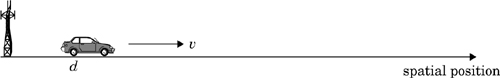
In Figure 5.2, the receiver moves along the ground at some constant velocity v. For a fixed position d, the channel between the transmitter and the receiver can be modeled as a linear time invariant system. However, due to the different multipath waves which have propagation delays which vary over different spatial locations of the receiver, the impulse response of the linear time invariant channel should be a function of the position of the receiver. That is, the channel impulse response can be expressed as h(d,t). Let x(t) represent the transmitted signal, then the received signal y(d,t) at position d can be expressed as a convolution of x(t) with h(d,t)
For a causal system, h(d,t) = 0 for t < 0, thus Equation (5.3) reduces to

Since the receiver moves along the ground at a constant velocity v, the position of the receiver can by expressed as
Substituting (5.5) in (5.4), we obtain
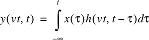
Since v is a constant, y(vt,t) is just a function of t. Therefore, Equation (5.6) can be expressed as

From Equation (5.7), it is clear that the mobile radio channel can be modeled as a linear time varying channel, where the channel changes with time and distance.
Since v may be assumed constant over a short time (or distance) interval, we may let x(t) represent the transmitted bandpass waveform, y(t) the received waveform, and h(t,τ) the impulse response of the time varying multipath radio channel. The impulse response h(t,τ) completely characterizes the channel and is a function of both t and τ. The variable t represents the time variations due to motion, whereas τ represents the channel multipath delay for a fixed value of t. One may think of τ as being a vernier adjustment of time. The received signal y(t) can be expressed as a convolution of the transmitted signal x(t) with the channel impulse response (see Figure 5.3a)
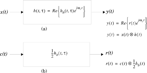
If the multipath channel is assumed to be a bandlimited bandpass channel, which is reasonable, then h(t,τ) may be equivalently described by a complex baseband impulse response hb(t,τ) with the input and output being the complex envelope representations of the transmitted and received signals, respectively (see Figure 5.3b). That is,
where c(t) and r(t) are the complex envelopes of x(t) and y(t), defined as
The factor of 1/2 in Equation (5.9) is due to the properties of the complex envelope, in order to represent the passband radio system at baseband. The lowpass characterization removes the high frequency variations caused by the carrier, making the signal analytically easier to handle. It is shown by Couch [Cou93] that the average power of a bandpass signal ![]() is equal to
is equal to ![]() , where the overbar denotes ensemble average for a stochastic signal, or time average for a deterministic or ergodic stochastic signal.
, where the overbar denotes ensemble average for a stochastic signal, or time average for a deterministic or ergodic stochastic signal.
It is useful to discretize the multipath delay axis τ of the impulse response into equal time delay segments called excess delay bins, where each bin has a time delay width equal to τi + 1 − τi, where τ0 is equal to 0, and represents the first arriving signal at the receiver. Letting i = 0, it is seen that τ1 − τ0 is equal to the time delay bin width given by Δτ. For convention, τ0 = 0, τ1 = Δτ, and τi = iΔτ, for i = 0 to N − 1, where N represents the total number of possible equally-spaced multipath components, including the first arriving component. Any number of multipath signals received within the ith bin are represented by a single resolvable multipath component having delay τi. This technique of quantizing the delay bins determines the time delay resolution of the channel model, and the useful frequency span of the model can be shown to be 2/Δτ. That is, the model may be used to analyze transmitted RF signals having bandwidths which are less than 2/Δτ. Note that τ0 = 0 is the excess time delay of the first arriving multipath component, and neglects the propagation delay between the transmitter and receiver. Excess delay is the relative delay of the ith multipath component as compared to the first arriving component and is given by τi. The maximum excess delay of the channel is given by NΔτ.
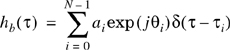
Since the received signal in a multipath channel consists of a series of attenuated, time-delayed, phase shifted replicas of the transmitted signal, the baseband impulse response of a multipath channel can be expressed as

where ai(t,τ) and τi(t) are the real amplitudes and excess delays, respectively, of ith multipath component at time t [Tur72]. The phase term 2πfc τi(t) + фi(t,τ) in (5.12) represents the phase shift due to free space propagation of the ith multipath component, plus any additional phase shifts which are encountered in the channel. In general, the phase term is simply represented by a single variable θi(t,τ) which lumps together all the mechanisms for phase shifts of a single multipath component within the ith excess delay bin. Note that some excess delay bins may have no multipath at some time t and delay τi, since ai(t,τ) may be zero. In Equation (5.12), N is the total possible number of multipath components (bins), and δ(•) is the unit impulse function which determines the specific multipath bins that have components at time t and excess delays τi. Figure 5.4 illustrates an example of different snapshots of hb(t,τ), where t varies into the page, and the time delay bins are quantized to widths of Δτ. Modern wireless communication systems have recently used spatial filtering to increase capacity and coverage, and often it is useful to modify Equation (5.12) to include the effects of angle of arrival of each multipath component [Lib99], [Ert98], [Mol01].
![An example of the time varying discrete-time impulse response model for a multipath radio channel. Discrete models are useful in simulation where modulation data must be convolved with the channel impulse response [Tra02].](http://imgdetail.ebookreading.net/system_admin/3/0130422320/0130422320__wireless-communications-principles__0130422320__graphics__05fig04.jpg)
Figure 5.4. An example of the time varying discrete-time impulse response model for a multipath radio channel. Discrete models are useful in simulation where modulation data must be convolved with the channel impulse response [Tra02].
It is important to note that depending on the choice of Δτ and the physical channel delay properties, there may be two or more multipath signals that arrive within an excess delay bin that are unresolvable and that vectorially combine to yield the instantaneous amplitude and phase of a single modeled multipath component. Such situations cause the multipath amplitude within an excess delay bin to fade over the local area. However, when only a single multipath component arrives within an excess delay bin, the amplitude over the local area for that particular time delay will generally not fade significantly.
If the channel impulse response is assumed to be time invariant, or is at least wide sense stationary over a small-scale time or distance interval, then the channel impulse response may be simplified as
The assumption of time invariance over a local area is valid when the time delay resolution of the channel impulse response model accurately and uniquely resolves every multipath component over the local area.
When measuring or predicting hb(τ), a probing pulse p(t) which approximates a delta function is used at the transmitter. That is,
is used to sound the channel to determine hb(τ).
For small-scale channel modeling, the power delay profile of the channel is found by taking the spatial average of ![]() over a local area. By making several local area measurements of
over a local area. By making several local area measurements of ![]() in different locations, it is possible to build an ensemble of power delay profiles, each one representing a possible small-scale multipath channel state [Rap91a].
in different locations, it is possible to build an ensemble of power delay profiles, each one representing a possible small-scale multipath channel state [Rap91a].
Based on work by Cox [Cox72], [Cox75], if p(t) has a time duration much smaller than the impulse response of the multipath channel, p(t) does not need to be deconvolved from the received signal r(t) in order to determine relative multipath signal strengths. The received power delay profile in a local area is given by
where the bar represents the average over the local area and many snapshots of ![]() are typically averaged over a local (small-scale) area to provide a single time-invariant multipath power delay profile P(τ). The gain k in Equation (5.15) relates the transmitted power in the probing pulse p(t) to the total power received in a multipath delay profile.
are typically averaged over a local (small-scale) area to provide a single time-invariant multipath power delay profile P(τ). The gain k in Equation (5.15) relates the transmitted power in the probing pulse p(t) to the total power received in a multipath delay profile.
In actual wireless communication systems, the impulse response of a multipath channel is measured in the field using channel sounding techniques. We now consider two extreme channel sounding cases as a means of demonstrating how the small-scale fading behaves quite differently for two signals with different bandwidths in the identical multipath channel.
Consider a pulsed, transmitted RF signal of the form
x(t) = Re{p(t)exp(j2πfct)} |
where p(t) is a repetitive baseband pulse train with very narrow pulse width Tbb and repetition period TREP which is much greater than the maximum measured excess delay τmax in the channel. Such a wideband pulse will produce an output that approximates hb(t,τ). Now let
and let p(t) be zero elsewhere for all excess delays of interest. The low pass channel output r(t) is found by convolving p(t) with hb(t,τ) and yields

To determine the received power at some time t0, the power |r(t0)|2 is measured. The quantity |r(t0)|2 is found by summing up the multipath powers resolved in the instantaneous multipath power delay profile |hb(t0;τ)|2 of the channel, and is equal to the energy received over the time duration of the multipath delay divided by τmax. That is, using Equation (5.16)
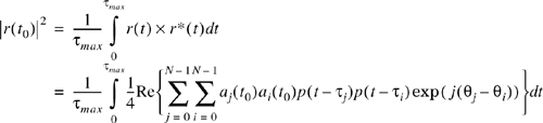
Note that if all the multipath components are resolved by the probe p(t), then ![]() for all j ≠ i, and
for all j ≠ i, and

For a wideband probing signal p(t), Tbb is smaller than the delays between multipath components in the channel, and Equation (5.18) shows that the total received power is simply related to the sum of the powers in the individual multipath components, and is scaled by the ratio of the probing pulse’s width and amplitude, and the maximum observed excess delay of the channel. Assuming that the received power from the multipath components forms a random process where each component has a random amplitude and phase at any time t, the average small-scale received power for the wideband probe is found from Equation (5.17) as
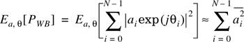
In Equation (5.19), Ea,θ[•] denotes the ensemble average over all possible values of ai and θi in a local area, and the overbar denotes sample average over a local measurement area which is generally measured using multipath measurement equipment. The striking result of Equations (5.18) and (5.19) is that if a transmitted signal is able to resolve the multipaths, then the average small-scale received power is simply the sum of the average powers received in each multipath component. In practice, the amplitudes of individual multipath components do not fluctuate widely in a local area. Thus, the received power of a wideband signal such as p(t) does not fluctuate significantly when a receiver is moved about a local area [Rap89].
Now, instead of a pulse, consider a CW signal which is transmitted into the exact same channel, and let the complex envelope be given by c(t) = 2. Then, the instantaneous complex envelope of the received signal is given by the phasor sum
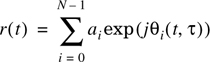
and the instantaneous power is given by

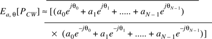
As the receiver is moved over a local area, the channel induces changes on r(t), and the received signal strength will vary at a rate governed by the fluctuations of ai and θi. As mentioned earlier, ai varies little over local areas, but θi will vary greatly due to changes in propagation distance over space, resulting in large fluctuations of r(t) as the receiver is moved over small distances (on the order of a wavelength). That is, since r(t) is the phasor sum of the individual multipath components, the instantaneous phases of the multipath components cause the large fluctuations which typifies small-scale fading for CW signals. The average received power over a local area is then given by

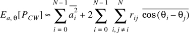
where rij is the path amplitude correlation coefficient defined to be
and the overbar denotes time average for CW measurements made by a mobile receiver over the local measurement area [Rap89]. Note that when ![]() and/or rij = 0, then the average power for a CW signal is equivalent to the average received power for a wideband signal in a small-scale region. This is seen by comparing Equation (5.19) and Equation (5.24). This can occur when either the multipath phases are identically and independently distributed (i.i.d uniform) over [0, 2π] or when the path amplitudes are uncorrelated. The i.i.d uniform distribution of θ is a valid assumption since multipath components traverse differential path lengths that measure hundreds of wavelengths and are likely to arrive with random phases. If for some reason it is believed that the phases are not independent, the average wideband power and average CW power will still be equal if the paths have uncorrelated amplitudes. However, if the phases of the paths are dependent upon each other, then the amplitudes are likely to be correlated, since the same mechanism which affects the path phases is likely to also affect the amplitudes. This situation is highly unlikely at transmission frequencies used in wireless mobile systems.
and/or rij = 0, then the average power for a CW signal is equivalent to the average received power for a wideband signal in a small-scale region. This is seen by comparing Equation (5.19) and Equation (5.24). This can occur when either the multipath phases are identically and independently distributed (i.i.d uniform) over [0, 2π] or when the path amplitudes are uncorrelated. The i.i.d uniform distribution of θ is a valid assumption since multipath components traverse differential path lengths that measure hundreds of wavelengths and are likely to arrive with random phases. If for some reason it is believed that the phases are not independent, the average wideband power and average CW power will still be equal if the paths have uncorrelated amplitudes. However, if the phases of the paths are dependent upon each other, then the amplitudes are likely to be correlated, since the same mechanism which affects the path phases is likely to also affect the amplitudes. This situation is highly unlikely at transmission frequencies used in wireless mobile systems.
Thus it is seen that the received local ensemble average power of wideband and narrowband signals are equivalent. When the transmitted signal has a bandwidth much greater than the bandwidth of the channel, then the multipath structure is completely resolved by the received signal at any time, and the received power varies very little since the individual multipath amplitudes do not change rapidly over a local area. However, if the transmitted signal has a very narrow bandwidth (e.g., the baseband signal has a duration greater than the excess delay of the channel), then multipath is not resolved by the received signal, and large signal fluctuations (fading) occur at the receiver due to the phase shifts of the many unresolved multipath components.
Figure 5.5 illustrates actual indoor radio channel measurements made simultaneously with a wideband probing pulse having Tbb = 10ns, and a CW transmitter. The carrier frequency was 4 GHz. It can be seen that the CW signal undergoes rapid fades, whereas the wideband measurements change little over the 5λ measurement track. However, the local average received powers of both signals were measured to be virtually identical [Haw91].
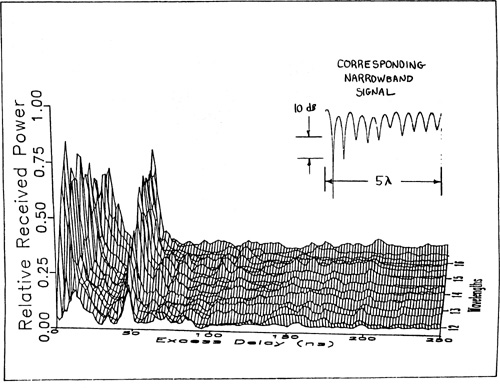
Figure 5.5. Measured wideband and narrowband received signals over a 5λ (0.375 m) measurement track inside a building. Carrier frequency is 4 GHz. Wideband power is computed using Equation (5.19), which can be thought of as the area under the power delay profile. The axis into the page is distance (wavelengths) instead of time.
Example 5.2.
Assume a discrete channel impulse response is used to model urban RF radio channels with excess delays as large as 100 μs and microcellular channels with excess delays no larger than 4 μs. If the number of multipath bins is fixed at 64, find (a) Δτ, and (b) the maximum RF bandwidth which the two models can accurately represent. Repeat the exercise for an indoor channel model with excess delays as large as 500 ns. As described in Section 5.7.6, SIRCIM and SMRCIM are statistical channel models based on Equation (5.12) that use parameters in this example.
Solution
The maximum excess delay of the channel model is given by τN = NΔτ. Therefore, for τN = 100 μs, and N = 64 we obtain Δτ = τN/N = 1.5625 μs. The maximum bandwidth that the SMRCIM model can accurately represent is equal to
2/Δτ = 2/1.5625 μs = 1.28 MHz. |
For the SMRCIM urban microcell model, τN = 4 μs, Δτ = τN/N = 62.5 ns. The maximum RF bandwidth that can be represented is
2/Δτ = 2/62.5 ns = 32 MHz. |
Similarly, for indoor channels, ![]() .
.
The maximum RF bandwidth for the indoor channel model is
2/Δτ = 2/7.8125 ns = 256 MHz. |
Example 5.3.
Assume a mobile traveling at a velocity of 10 m/s receives two multipath components at a carrier frequency of 1000 MHz. The first component is assumed to arrive at τ = 0 with an initial phase of 0° and a power of –70 dBm, and the second component which is 3 dB weaker than the first component is assumed to arrive at τ = 1 μs, also with an initial phase of 0°. If the mobile moves directly toward the direction of arrival of the first component and directly away from the direction of arrival of the second component, compute the narrowband instantaneous power at time intervals of 0.1 s from 0 s to 0.5 s. Compute the average narrowband power received over this observation interval. Compare average narrowband and wideband received powers over the interval, assuming the amplitudes of the two multipath components do not fade over the local area.
Solution
Given v = 10 m/s, time intervals of 0.1 s correspond to spatial intervals of 1 m. The carrier frequency is given to be 1000 MHz, hence the wavelength of the signal is
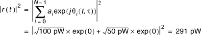
The narrowband instantaneous power can be computed using Equation (5.21).
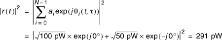
Note –70 dBm = 100 pW. At time t = 0, the phases of both multipath components are 0°, hence the narrowband instantaneous power is equal to
Now, as the mobile moves, the phase of the two multipath components changes in opposite directions.
At t = 0.1 s, the phase of the first component is
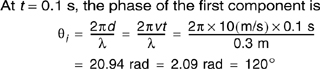
Since the mobile moves toward the direction of arrival of the first component, and away from the direction of arrival of the second component, θ1 is positive, and θ2 is negative.
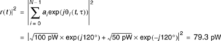
Therefore, at t = 0.1 s, θ1 = 120°, and θ2 = −120°, and the instantaneous power is equal to
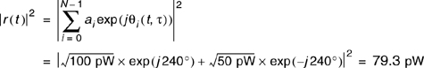
Similarly, at t = 0.2 s, θ1 = 240°, and θ2 = –240°, and the instantaneous power is equal to
Similarly, at t = 0.3 s, θ1 = 360° = 0°, and θ2 = −360° = 0°, and the instantaneous power is equal to
It follows that at t = 0.4 s, |r(t)|2 = 79.3pW, and at t = 0.5 s, |r(t)|2 = 79.3 pW. The average narrowband received power is equal to
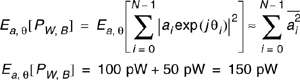
Using Equation (5.19), the wideband power is given by
As can be seen, the narrowband and wideband received power are virtually identical when averaged over 0.5 s (or 5 m). While the CW signal fades over the observation interval, the wideband signal power remains constant over the same spatial interval.
Because of the importance of the multipath structure in determining the small-scale fading effects, a number of wideband channel sounding techniques have been developed. These techniques may be classified as direct pulse measurements, spread spectrum sliding correlator measurements, and swept frequency measurements.
A simple channel sounding approach is the direct RF pulse system (see Figure 5.6). This technique allows engineers to determine rapidly the power delay profile of any channel, as demonstrated by Rappaport and Seidel [Rap89], [Rap90]. Essentially a wideband pulsed bistatic radar, this system transmits a repetitive pulse of width Tbb s, and uses a receiver with a wide bandpass filter (BW = 2/TbbHz). The signal is then amplified, detected with an envelope detector, and displayed and stored on a high speed oscilloscope. This gives an immediate measurement of the square of the channel impulse response convolved with the probing pulse (see Equation (5.17)). If the oscilloscope is set on averaging mode, then this system can provide a local average power delay profile. Another attractive aspect of this system is the lack of complexity, since off-the-shelf equipment may be used.
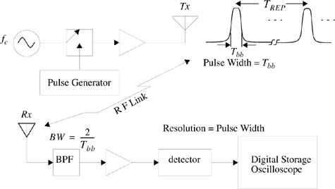
The minimum resolvable delay between multipath components is equal to the probing pulse width Tbb. The main problem with this system is that it is subject to interference and noise, due to the wide passband filter required for multipath time resolution. Also, the pulse system relies on the ability to trigger the oscilloscope on the first arriving signal. If the first arriving signal is blocked or fades, severe fading occurs, and it is possible the system may not trigger properly. Another disadvantage is that the phases of the individual multipath components are not received, due to the use of an envelope detector. However, use of a coherent detector permits measurement of the multipath phase using this technique.
The basic block diagram of a spread spectrum channel sounding system is shown in Figure 5.7. The advantage of a spread spectrum system is that, while the probing signal may be wideband, it is possible to detect the transmitted signal using a narrowband receiver preceded by a wideband mixer, thus improving the dynamic range of the system as compared to the direct RF pulse system.
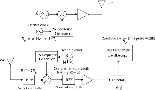
In a spread spectrum channel sounder, a carrier signal is “spread” over a large bandwidth by mixing it with a binary pseudo-noise (PN) sequence having a chip duration Tc and a chip rate Rc equal to 1/Tc Hz. The power spectrum envelope of the transmitted spread spectrum signal is given by [Dix84] as
and the null-to-null RF bandwidth is
The spread spectrum signal is then received, filtered, and despread using a PN sequence generator identical to that used at the transmitter. Although the two PN sequences are identical, the transmitter chip clock is run at a slightly faster rate than the receiver chip clock. Mixing the chip sequences in this fashion implements a sliding correlator [Dix84]. When the PN code of the faster chip clock catches up with the PN code of the slower chip clock, the two chip sequences will be virtually identically aligned, giving maximal correlation. When the two sequences are not maximally correlated, mixing the incoming spread spectrum signal with the unsynchronized receiver chip sequence will spread this signal into a bandwidth at least as large as the receiver’s reference PN sequence. In this way, the narrowband filter that follows the correlator can reject almost all of the incoming signal power. This is how processing gain is realized in a spread spectrum receiver and how it can reject passband interference, unlike the direct RF pulse sounding system.
Processing gain (PG) is given as
where Tbb = 1/Rbb, is the period of the baseband information. For the case of a sliding correlator channel sounder, the baseband information rate is equal to the frequency offset of the PN sequence clocks at the transmitter and receiver.
When the incoming signal is correlated with the receiver sequence, the signal is collapsed back to the original bandwidth (i.e., “despread”), envelope detected, and displayed on an oscilloscope. Since different incoming multipaths will have different time delays, they will maximally correlate with the receiver PN sequence at different times. The energy of these individual paths will pass through the correlator depending on the time delay. Therefore, after envelope detection, the channel impulse response convolved with the pulse shape of a single chip is displayed on the oscilloscope. Cox [Cox72] first used this method to measure channel impulse responses in outdoor suburban environments at 910 MHz. Devasirvatham [Dev86], [Dev90a] successfully used a direct sequence spread spectrum channel sounder to measure time delay spread of multipath components and signal level measurements in office and residential buildings at 850 MHz. Bultitude [Bul89] used this technique for indoor and microcellular channel sounding work, as did Landron [Lan92], while Newhall and Saldanha measured campuses and train yards [New96a]. A detailed description of a practical sliding correlator is given in [New96b].
The time resolution (Δτ) of multipath components using a spread spectrum system with sliding correlation is
In other words, the system can resolve two multipath components as long as they are equal to or greater than two chip durations, or 2Tc seconds apart. In actuality, multipath components with interarrival times smaller than 2Tc can be resolved since the rms pulse width of a chip is smaller than the absolute width of the triangular correlation pulse, and is on the order of Tc.
The sliding correlation process gives equivalent time measurements that are updated every time the two sequences are maximally correlated. The time between maximal correlations (ΔT) can be calculated from Equation (5.30)
where Tc | = | chip period (s) |
Rc | = | chip rate (Hz) |
γ | = | slide factor (dimensionless) |
l | = | sequence length (chips) |
The slide factor is defined as the ratio between the transmitter chip clock rate and the difference between the transmitter and receiver chip clock rates [Dev86]. Mathematically, this is expressed as
where α | = | transmitter chip clock rate (Hz) |
β | = | receiver chip clock rate (Hz) |
For a maximal length PN sequence, the sequence length is
where n is the number of shift registers in the sequence generator [Dix84].
Since the incoming spread spectrum signal is mixed with a receiver PN sequence that is slower than the transmitter sequence, the signal is essentially down-converted (“collapsed”) to a low-frequency narrowband signal. In other words, the relative rate of the two codes slipping past each other is the rate of information transferred to the oscilloscope. This narrowband signal allows narrowband processing, eliminating much of the passband noise and interference. The processing gain of Equation (5.28) is then realized using a narrowband filter (BW = 2(α − β)).
The equivalent time measurements refer to the relative times of multipath components as they are displayed on the oscilloscope. The observed time scale on the oscilloscope using a sliding correlator is related to the actual propagation time scale by
This effect is due to the relative rate of information transfer in the sliding correlator. For example, ΔT of Equation (5.30) is an observed time measured on an oscilloscope and not actual propagation time. This effect, known as time dilation, occurs in the sliding correlator system because the propagation delays are actually expanded in time by the sliding correlator.
Caution must be taken to ensure that the sequence length has a period which is greater than the longest multipath propagation delay. The PN sequence period is
The sequence period gives an estimate of the maximum unambiguous range of incoming multipath signal components. This range is found by multiplying the speed of light with τPNseq in Equation (5.34).
There are several advantages to the spread spectrum channel sounding system. One of the key spread spectrum modulation characteristics is the ability to reject passband noise, thus improving the coverage range for a given transmitter power. Transmitter and receiver PN sequence synchronization is eliminated by the sliding correlator. Sensitivity is adjustable by changing the sliding factor and the post-correlator filter bandwidth. Also, required transmitter powers can be considerably lower than comparable direct pulse systems due to the inherent “processing gain” of spread spectrum systems.
A disadvantage of the spread spectrum system, as compared to the direct pulse system, is that measurements are not made in real time, but they are compiled as the PN codes slide past one another. Depending on system parameters and measurement objectives, the time required to make power delay profile measurements may be excessive. Another disadvantage of the system described here is that a noncoherent detector is used, so that phases of individual multipath components can not be measured. Even if coherent detection is used, the sweep time of a spread spectrum signal induces delay such that the phases of individual multipath components with different time delays would be measured at substantially different times, during which the channel might change.
Because of the dual relationship between time domain and frequency domain techniques, it is possible to measure the channel impulse response in the frequency domain. Figure 5.8 shows a frequency domain channel sounder used for measuring channel impulse responses. A vector network analyzer controls a synthesized frequency sweeper, and an S-parameter test set is used to monitor the frequency response of the channel. The sweeper scans a particular frequency band (centered on the carrier) by stepping through discrete frequencies. The number and spacings of these frequency steps impact the time resolution of the impulse response measurement. For each frequency step, the S-parameter test set transmits a known signal level at port 1 and monitors the received signal level at port 2. These signal levels allow the analyzer to determine the complex response (i.e., transmissivity S21(ω)) of the channel over the measured frequency range. The transmissivity response is a frequency domain representation of the channel impulse response. This response is then converted to the time domain using inverse discrete Fourier transform (IDFT) processing, giving a band-limited version of the impulse response. In theory, this technique works well and indirectly provides amplitude and phase information in the time domain. However, the system requires careful calibration and hardwired synchronization between the transmitter and receiver, making it useful only for very close measurements (e.g., indoor channel sounding). Another limitation with this system is the non-real-time nature of the measurement. For time varying channels, the channel frequency response can change rapidly, giving an erroneous impulse response measurement. To mitigate this effect, fast sweep times are necessary to keep the total swept frequency response measurement interval as short as possible. A faster sweep time can be accomplished by reducing the number of frequency steps, but this sacrifices time resolution and excess delay range in the time domain. The swept frequency system has been used successfully for indoor propagation studies by Pahlavan [Pah95] and Zaghloul et al. [Zag91a], [Zag91b].

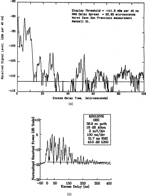
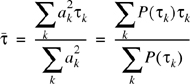
Many multipath channel parameters are derived from the power delay profile, given by Equation (5.18). Power delay profiles are measured using the techniques discussed in Section 5.4 and are generally represented as plots of relative received power as a function of excess delay with respect to a fixed time delay reference. Power delay profiles are found by averaging instantaneous power delay profile measurements over a local area in order to determine an average small-scale power delay profile. Depending on the time resolution of the probing pulse and the type of multipath channels studied, researchers often choose to sample at spatial separations of a quarter of a wavelength and over receiver movements no greater than 6 m in outdoor channels and no greater than 2 m in indoor channels in the 450 MHz–6 GHz range. This small-scale sampling avoids large-scale averaging bias in the resulting small-scale statistics. Figure 5.9 shows typical power delay profile plots from outdoor and indoor channels, determined from a large number of closely sampled instantaneous profiles.
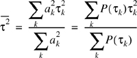
In order to compare different multipath channels and to develop some general design guidelines for wireless systems, parameters which grossly quantify the multipath channel are used. The mean excess delay, rms delay spread, and excess delay spread (X dB) are multipath channel parameters that can be determined from a power delay profile. The time dispersive properties of wide band multipath channels are most commonly quantified by their mean excess delay ![]() and rms delay spread (στ). The mean excess delay is the first moment of the power delay profile and is defined to be
and rms delay spread (στ). The mean excess delay is the first moment of the power delay profile and is defined to be
The rms delay spread is the square root of the second central moment of the power delay profile and is defined to be
where
These delays are measured relative to the first detectable signal arriving at the receiver at τ0 = 0. Equations (5.35)–(5.37) do not rely on the absolute power level of P(τ), but only the relative amplitudes of the multipath components within P(τ). Typical values of rms delay spread are on the order of microseconds in outdoor mobile radio channels and on the order of nanoseconds in indoor radio channels. Table 5.1 shows the typical measured values of rms delay spread.
Table 5.1. Typical Measured Values of RMS Delay Spread
Environment | Frequency (MHz) | RMS Delay Spread (στ) | Notes | Reference |
|---|---|---|---|---|
Urban | 910 | 1300 ns avg. 600 ns st. dev. 3500 ns max. | New York City | |
Urban | 892 | 10–25 μs | Worst case San Francisco | |
Suburban | 910 | 200–310 ns | Averaged typical case | |
Suburban | 910 | 1960–2110 ns | Averaged extreme case | |
Indoor | 1500 | 10–50 ns 25 ns median | Office building | |
Indoor | 850 | 270 ns max. | Office building | |
Indoor | 1900 | 70–94 ns avg. 1470 ns max. | Three San Francisco buildings |
It is important to note that the rms delay spread and mean excess delay are defined from a single power delay profile which is the temporal or spatial average of consecutive impulse response measurements collected and averaged over a local area. Typically, many measurements are made at many local areas in order to determine a statistical range of multipath channel parameters for a mobile communication system over a large-scale area [Rap90].
The maximum excess delay (X dB) of the power delay profile is defined to be the time delay during which multipath energy falls to X dB below the maximum. In other words, the maximum excess delay is defined as τX − τ0, where τ0 is the first arriving signal and τX is the maximum delay at which a multipath component is within X dB of the strongest arriving multipath signal (which does not necessarily arrive at τ0). Figure 5.10 illustrates the computation of the maximum excess delay for multipath components within 10 dB of the maximum. The maximum excess delay (X dB) defines the temporal extent of the multipath that is above a particular threshold. The value of τX is sometimes called the excess delay spread of a power delay profile, but in all cases must be specified with a threshold that relates the multipath noise floor to the maximum received multipath component.
In practice, values for ![]() ,
, ![]() , and στ depend on the choice of noise threshold used to process P(τ). The noise threshold is used to differentiate between received multipath components and thermal noise. If the noise threshold is set too low, then noise will be processed as multipath, thus giving rise to values of
, and στ depend on the choice of noise threshold used to process P(τ). The noise threshold is used to differentiate between received multipath components and thermal noise. If the noise threshold is set too low, then noise will be processed as multipath, thus giving rise to values of ![]() ,
, ![]() , and στ that are artificially high.
, and στ that are artificially high.
It should be noted that the power delay profile and the magnitude frequency response (the spectral response) of a mobile radio channel are related through the Fourier transform. It is therefore possible to obtain an equivalent description of the channel in the frequency domain using its frequency response characteristics. Analogous to the delay spread parameters in the time domain, coherence bandwidth is used to characterize the channel in the frequency domain. The rms delay spread and coherence bandwidth are inversely proportional to one another, although their exact relationship is a function of the exact multipath structure.

While the delay spread is a natural phenomenon caused by reflected and scattered propagation paths in the radio channel, the coherence bandwidth, Bc, is a defined relation derived from the rms delay spread. Coherence bandwidth is a statistical measure of the range of frequencies over which the channel can be considered “flat” (i.e., a channel which passes all spectral components with approximately equal gain and linear phase). In other words, coherence bandwidth is the range of frequencies over which two frequency components have a strong potential for amplitude correlation. Two sinusoids with frequency separation greater than Bc are affected quite differently by the channel. If the coherence bandwidth is defined as the bandwidth over which the frequency correlation function is above 0.9, then the coherence bandwidth is approximately [Lee89b]
If the definition is relaxed so that the frequency correlation function is above 0.5, then the coherence bandwidth is approximately
It is important to note that an exact relationship between coherence bandwidth and rms delay spread is a funtion of specific channel impulse responses and applied signals, and Equations (5.38) and (5.39) are “ball park estimates.” In general, spectral analysis techniques and simulation are required to determine the exact impact that time varying multipath has on a particular transmitted signal [Chu87], [Fun93], [Ste94]. For this reason, accurate multipath channel models must be used in the design of specific modems for wireless applications [Rap91a], [Woe94].
Example 5.5.
Calculate the mean excess delay, rms delay spread, and the maximum excess delay (10 dB) for the multipath profile given in the figure below. Estimate the 50% coherence bandwidth of the channel. Would this channel be suitable for AMPS or GSM service without the use of an equalizer?

Solution
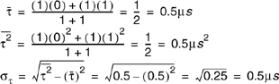
Using the definition of maximum excess delay (10 dB), it can be seen that τ10 dB is 5 μs. The rms delay spread for the given multipath profile can be obtained using Equations (5.35)–(5.37). The delays of each profile are measured relative to the first detectable signal. The mean excess delay for the given profile is
The second moment for the given power delay profile can be calculated as
Therefore the rms delay spread is ![]()
The coherence bandwidth is found from Equation (5.39) to be
Since Bc is greater than 30 kHz, AMPS will work without an equalizer. However, GSM requires 200 kHz bandwidth which exceeds Bc, thus an equalizer would be needed for this channel.
Delay spread and coherence bandwidth are parameters which describe the time dispersive nature of the channel in a local area. However, they do not offer information about the time varying nature of the channel caused by either relative motion between the mobile and base station, or by movement of objects in the channel. Doppler spread and coherence time are parameters which describe the time varying nature of the channel in a small-scale region.
Doppler spread BD is a measure of the spectral broadening caused by the time rate of change of the mobile radio channel and is defined as the range of frequencies over which the received Doppler spectrum is essentially non-zero. When a pure sinusoidal tone of frequency fc is transmitted, the received signal spectrum, called the Doppler spectrum, will have components in the range fc − fd to fc + fd, where fd is the Doppler shift. The amount of spectral broadening depends on fd which is a function of the relative velocity of the mobile, and the angle θ between the direction of motion of the mobile and direction of arrival of the scattered waves. If the baseband signal bandwidth is much greater than BD, the effects of Doppler spread are negligible at the receiver. This is a slow fading channel.
Coherence time Tc is the time domain dual of Doppler spread and is used to characterize the time varying nature of the frequency dispersiveness of the channel in the time domain. The Doppler spread and coherence time are inversely proportional to one another. That is,
Coherence time is actually a statistical measure of the time duration over which the channel impulse response is essentially invariant, and quantifies the similarity of the channel response at different times. In other words, coherence time is the time duration over which two received signals have a strong potential for amplitude correlation. If the reciprocal bandwidth of the baseband signal is greater than the coherence time of the channel, then the channel will change during the transmission of the baseband message, thus causing distortion at the receiver. If the coherence time is defined as the time over which the time correlation function is above 0.5, then the coherence time is approximately [Ste94]
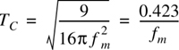
where fm is the maximum Doppler shift given by fm = v/λ. In practice, (5.40.a) suggests a time duration during which a Rayleigh fading signal may fluctuate wildly, and (5.40.b) is often too restrictive. A popular rule of thumb for modern digital communications is to define the coherence time as the geometric mean of Equations (5.40.a) and (5.40.b). That is,
The definition of coherence time implies that two signals arriving with a time separation greater than TC are affected differently by the channel. For example, for a vehicle traveling 60 mph using a 900 MHz carrier, a conservative value of TC can be shown to be 2.22 ms from Equation (5.40.b). If a digital transmission system is used, then as long as the symbol rate is greater than 1/TC = 454 bps, the channel will not cause distortion due to motion (however, distortion could result from multipath time delay spread, depending on the channel impulse response). Using the practical formula of (5.40.c), TC = 6.77 ms and the symbol rate must exceed 150 bits/s in order to avoid distortion due to frequency dispersion.
Example 5.6.
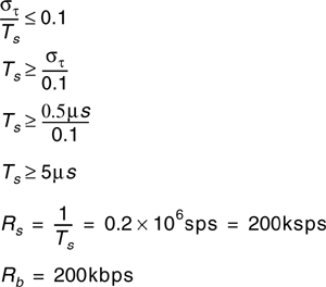
Determine the proper spatial sampling interval required to make small-scale propagation measurements which assume that consecutive samples are highly correlated in time. How many samples will be required over 10 m travel distance if fc = 1900 MHz and v = 50 m/s. How long would it take to make these measurements, assuming they could be made in real time from a moving vehicle? What is the Doppler spread BD for the channel?
Solution
For correlation, ensure that the time between samples is equal to TC/2, and use the smallest value of TC for conservative design.
Using Equation (5.40.b)

Taking time samples at less than half TC, at 282.5 μs corresponds to a spatial sampling interval of
Therefore, the number of samples required over a 10 m travel distance is
The time taken to make this measurement is equal to ![]()
The Doppler spread is ![]()
Section 5.3 demonstrated that the type of fading experienced by a signal propagating through a mobile radio channel depends on the nature of the transmitted signal with respect to the characteristics of the channel. Depending on the relation between the signal parameters (such as bandwidth, symbol period, etc.) and the channel parameters (such as rms delay spread and Doppler spread), different transmitted signals will undergo different types of fading. The time dispersion and frequency dispersion mechanisms in a mobile radio channel lead to four possible distinct effects, which are manifested depending on the nature of the transmitted signal, the channel, and the velocity. While multipath delay spread leads to time dispersion and frequency selective fading, Doppler spread leads to frequency dispersion and time selective fading. The two propagation mechanisms are independent of one another. Figure 5.11 shows a tree of the four different types of fading.
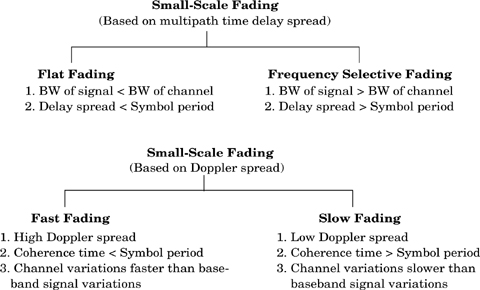
Time dispersion due to multipath causes the transmitted signal to undergo either flat or frequency selective fading.
If the mobile radio channel has a constant gain and linear phase response over a bandwidth which is greater than the bandwidth of the transmitted signal, then the received signal will undergo flat fading. This type of fading is historically the most common type of fading described in the technical literature. In flat fading, the multipath structure of the channel is such that the spectral characteristics of the transmitted signal are preserved at the receiver. However the strength of the received signal changes with time, due to fluctuations in the gain of the channel caused by multipath. The characteristics of a flat fading channel are illustrated in Figure 5.12.
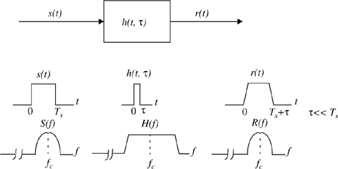
It can be seen from Figure 5.12 that if the channel gain changes over time, a change of amplitude occurs in the received signal. Over time, the received signal r(t) varies in gain, but the spectrum of the transmission is preserved. In a flat fading channel, the reciprocal bandwidth of the transmitted signal is much larger than the multipath time delay spread of the channel, and hb(t,τ) can be approximated as having no excess delay (i.e., a single delta function with τ = 0). Flat fading channels are also known as amplitude varying channels and are sometimes referred to as narrowband channels, since the bandwidth of the applied signal is narrow as compared to the channel flat fading bandwidth. Typical flat fading channels cause deep fades, and thus may require 20 or 30 dB more transmitter power to achieve low bit error rates during times of deep fades as compared to systems operating over non-fading channels. The distribution of the instantaneous gain of flat fading channels is important for designing radio links, and the most common amplitude distribution is the Rayleigh distribution. The Rayleigh flat fading channel model assumes that the channel induces an amplitude which varies in time according to the Rayleigh distribution.
To summarize, a signal undergoes flat fading if
and
where TS is the reciprocal bandwidth (e.g., symbol period) and BS is the bandwidth, respectively, of the transmitted modulation, and στ and BC are the rms delay spread and coherence bandwidth, respectively, of the channel.
If the channel possesses a constant-gain and linear phase response over a bandwidth that is smaller than the bandwidth of transmitted signal, then the channel creates frequency selective fading on the received signal. Under such conditions, the channel impulse response has a multipath delay spread which is greater than the reciprocal bandwidth of the transmitted message waveform. When this occurs, the received signal includes multiple versions of the transmitted waveform which are attenuated (faded) and delayed in time, and hence the received signal is distorted. Frequency selective fading is due to time dispersion of the transmitted symbols within the channel. Thus the channel induces intersymbol interference (ISI). Viewed in the frequency domain, certain frequency components in the received signal spectrum have greater gains than others.
Frequency selective fading channels are much more difficult to model than flat fading channels since each multipath signal must be modeled and the channel must be considered to be a linear filter. It is for this reason that wideband multipath measurements are made, and models are developed from these measurements. When analyzing mobile communication systems, statistical impulse response models such as the two-ray Rayleigh fading model (which considers the impulse response to be made up of two delta functions which independently fade and have sufficient time delay between them to induce frequency selective fading upon the applied signal), or computer generated or measured impulse responses, are generally used for analyzing frequency selective small-scale fading. Figure 5.13 illustrates the characteristics of a frequency selective fading channel.
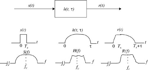
For frequency selective fading, the spectrum S(f) of the transmitted signal has a bandwidth which is greater than the coherence bandwidth BC of the channel. Viewed in the frequency domain, the channel becomes frequency selective, where the gain is different for different frequency components. Frequency selective fading is caused by multipath delays which approach or exceed the symbol period of the transmitted symbol. Frequency selective fading channels are also known as wideband channels since the bandwidth of the signal s(t) is wider than the bandwidth of the channel impulse response. As time varies, the channel varies in gain and phase across the spectrum of s(t), resulting in time varying distortion in the received signal r(t). To summarize, a signal undergoes frequency selective fading if
and
A common rule of thumb is that a channel is flat fading if Ts ≥ 10 στ and a channel is frequency selective if Ts < 10 στ, although this is dependent on the specific type of modulation used. Chapter 6 presents simulation results which illustrate the impact of time delay spread on bit error rate (BER).
Depending on how rapidly the transmitted baseband signal changes as compared to the rate of change of the channel, a channel may be classified either as a fast fading or slow fading channel. In a fast fading channel, the channel impulse response changes rapidly within the symbol duration. That is, the coherence time of the channel is smaller than the symbol period of the transmitted signal. This causes frequency dispersion (also called time selective fading) due to Doppler spreading, which leads to signal distortion. Viewed in the frequency domain, signal distortion due to fast fading increases with increasing Doppler spread relative to the bandwidth of the transmitted signal. Therefore, a signal undergoes fast fading if
and
It should be noted that when a channel is specified as a fast or slow fading channel, it does not specify whether the channel is flat fading or frequency selective in nature. Fast fading only deals with the rate of change of the channel due to motion. In the case of the flat fading channel, we can approximate the impulse response to be simply a delta function (no time delay). Hence, a flat fading, fast fading channel is a channel in which the amplitude of the delta function varies faster than the rate of change of the transmitted baseband signal. In the case of a frequency selective, fast fading channel, the amplitudes, phases, and time delays of any one of the multipath components vary faster than the rate of change of the transmitted signal. In practice, fast fading only occurs for very low data rates.
In a slow fading channel, the channel impulse response changes at a rate much slower than the transmitted baseband signal s(t). In this case, the channel may be assumed to be static over one or several reciprocal bandwidth intervals. In the frequency domain, this implies that the Doppler spread of the channel is much less than the bandwidth of the baseband signal. Therefore, a signal undergoes slow fading if
and
It should be clear that the velocity of the mobile (or velocity of objects in the channel) and the baseband signaling determines whether a signal undergoes fast fading or slow fading.
The relation between the various multipath parameters and the type of fading experienced by the signal are summarized in Figure 5.14. Over the years, some authors have confused the terms fast and slow fading with the terms large-scale and small-scale fading. It should be emphasized that fast and slow fading deal with the relationship between the time rate of change in the channel and the transmitted signal, and not with propagation path loss models.

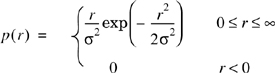
In mobile radio channels, the Rayleigh distribution is commonly used to describe the statistical time varying nature of the received envelope of a flat fading signal, or the envelope of an individual multipath component. It is well known that the envelope of the sum of two quadrature Gaussian noise signals obeys a Rayleigh distribution. Figure 5.15 shows a Rayleigh distributed signal envelope as a function of time. The Rayleigh distribution has a probability density function (pdf) given by
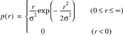

where σ is the rms value of the received voltage signal before envelope detection, and σ2 is the time-average power of the received signal before envelope detection. The probability that the envelope of the received signal does not exceed a specified value R is given by the corresponding cumulative distribution function (CDF)
The mean value rmean of the Rayleigh distribution is given by

and the variance of the Rayleigh distribution is given by ![]() , which represents the ac power in the signal envelope
, which represents the ac power in the signal envelope

The rms value of the envelope is the square root of the mean square, or ![]() , where σ is the standard deviation of the original complex Gaussian signal prior to envelope detection.
, where σ is the standard deviation of the original complex Gaussian signal prior to envelope detection.
The median value of r is found by solving
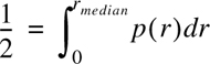
and is
Thus the mean and the median differ by only 0.55 dB in a Rayleigh fading signal. Note that the median is often used in practice, since fading data are usually measured in the field and a particular distribution cannot be assumed. By using median values instead of mean values, it is easy to compare different fading distributions which may have widely varying means. Figure 5.16 illustrates the Rayleigh pdf. The corresponding Rayleigh cumulative distribution function (CDF) is shown in Figure 5.17.

When there is a dominant stationary (nonfading) signal component present, such as a line-of-sight propagation path, the small-scale fading envelope distribution is Ricean. In such a situation, random multipath components arriving at different angles are superimposed on a stationary dominant signal. At the output of an envelope detector, this has the effect of adding a dc component to the random multipath.
Just as for the case of detection of a sine wave in thermal noise [Ric48], the effect of a dominant signal arriving with many weaker multipath signals gives rise to the Ricean distribution. As the dominant signal becomes weaker, the composite signal resembles a noise signal which has an envelope that is Rayleigh. Thus, the Ricean distribution degenerates to a Rayleigh distribution when the dominant component fades away.
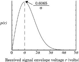
The Ricean distribution is given by
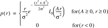
The parameter A denotes the peak amplitude of the dominant signal and I0(•) is the modified Bessel function of the first kind and zero-order. The Ricean distribution is often described in terms of a parameter K which is defined as the ratio between the deterministic signal power and the variance of the multipath. It is given by K = A2/(2σ2) or, in terms of dB
The parameter K is known as the Ricean factor and completely specifies the Ricean distribution. As A → 0, K → –∞ dB, and as the dominant path decreases in amplitude, the Ricean distribution degenerates to a Rayleigh distribution. Figure 5.18 shows the Ricean pdf. The Ricean CDF is compared with the Rayleigh CDF in Figure 5.17.

Several multipath models have been suggested to explain the observed statistical nature of a mobile channel. The first model presented by Ossana [Oss64] was based on interference of waves incident and reflected from the flat sides of randomly located buildings. Although Ossana’s model [Oss64] predicts flat fading power spectra that were in agreement with measurements in suburban areas, it assumes the existence of a direct path between the transmitter and receiver, and is limited to a restricted range of reflection angles. Ossana’s model is therefore rather inflexible and inappropriate for urban areas where the direct path is almost always blocked by buildings or other obstacles. Clarke’s model [Cla68] is based on scattering and is widely used.
Clarke [Cla68] developed a model where the statistical characteristics of the electromagnetic fields of the received signal at the mobile are deduced from scattering. The model assumes a fixed transmitter with a vertically polarized antenna. The field incident on the mobile antenna is assumed to be comprised of N azimuthal plane waves with arbitrary carrier phases, arbitrary azimuthal angles of arrival, and each wave having equal average amplitude. It should be noted that the equal average amplitude assumption is based on the fact that in the absence of a direct line-of-sight path, the scattered components arriving at a receiver will experience similar attenuation over small-scale distances.
Figure 5.19 shows a diagram of plane waves incident on a mobile traveling at a velocity v, in the x-direction. The angle of arrival is measured in the x-y plane with respect to the direction of motion. Every wave that is incident on the mobile undergoes a Doppler shift due to the motion of the receiver and arrives at the receiver at the same time. That is, no excess delay due to multipath is assumed for any of the waves (flat fading assumption). For the nth wave arriving at an angle αn to the x-axis, the Doppler shift in Hertz is given by
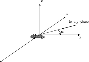
where λ is the wavelength of the incident wave.
The vertically polarized plane waves arriving at the mobile have E and H field components given by
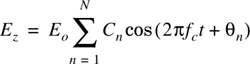
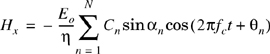

where E0 is the real amplitude of local average E-field (assumed constant), Cn is a real random variable representing the amplitude of individual waves, η is the intrinsic impedance of free space (377Ω), and fc is the carrier frequency. The random phase of the nth arriving component θn is given by
The amplitudes of the E-and H-field are normalized such that the ensemble average of the Cn ’s is given by

Since the Doppler shift is very small when compared to the carrier frequency, the three field components may be modeled as narrow band random processes. The three components Ez, Hx, and Hy can be approximated as Gaussian random variables if N is sufficiently large. The phase angles are assumed to have a uniform probability density function (pdf) on the interval (0,2π]. Based on the analysis by Rice [Ric48] the E-field can be expressed in an in-phase and quadrature form
where
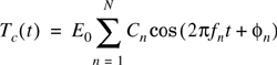
and
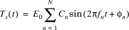
Both Tc(t) and Ts(t) are Gaussian random processes which are denoted as Tc and Ts, respectively, at any time t. Tc and Ts are uncorrelated zero-mean Gaussian random variables with an equal variance given by
where the overbar denotes the ensemble average.
The envelope of the received E-field, Ez(t), is given by
Since Tc and Ts are Gaussian random variables, it can be shown through a Jacobean transformation [Pap91] that the random received signal envelope r has a Rayleigh distribution given by
where ![]() .
.
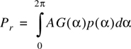
Gans [Gan72] developed a spectrum analysis for Clarke’s model. Let p(α)dα denote the fraction of the total incoming power within dα of the angle α, and let A denote the average received power with respect to an isotropic antenna. As N → ∞, p(α)dα approaches a continuous, rather than a discrete, distribution. If G(α) is the azimuthal gain pattern of the mobile antenna as a function of the angle of arrival, the total received power can be expressed as
where AG(α)p(α)dα is the differential variation of received power with angle. If the scattered signal is a CW signal of frequency fc, then the instantaneous frequency of the received signal component arriving at an angle α is obtained using Equation (5.57)
where fm is the maximum Doppler shift. It should be noted that f(α) is an even function of α, (i.e., f(α) = f(−α)).
If S(f) is the power spectrum of the received signal, the differential variation of received power with frequency is given by
Equating the differential variation of received power with frequency to the differential variation in received power with angle, we have
Differentiating Equation (5.70), and rearranging the terms, we have
Using Equation (5.70), α can be expressed as a function of f as
This implies that

Substituting Equation (5.73) and (5.75) into both sides of (5.72), the power spectral density S(f) can be expressed as

where
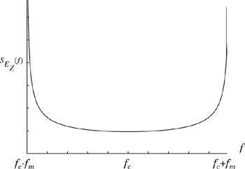
The spectrum is centered on the carrier frequency and is zero outside the limits of fc ± fm. Each of the arriving waves has its own carrier frequency (due to its direction of arrival) which is slightly offset from the center frequency. For the case of a vertical λ/4 antenna (G(α) = 1.5), and a uniform distribution p(α) = 1/2π over 0 to 2π, the output spectrum is given by (5.76) as
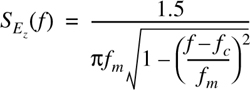
In Equation (5.78), the power spectral density at f = fc ± fm is infinite, i.e., Doppler components arriving at exactly 0° and 180° have an infinite power spectral density. This is not a problem since α is continuously distributed and the probability of components arriving at exactly these angles is zero.
Figure 5.20 shows the power spectral density of the resulting RF signal due to Doppler fading. Smith [Smi75] demonstrated an easy way to simulate Clarke’s model using a computer simulation as described Section 5.7.2.
After envelope detection of the Doppler-shifted signal, the resulting baseband spectrum has a maximum frequency of 2fm. It can be shown [Jak74] that the electric field produces a baseband power spectral density given by
where K[•] is the complete elliptical integral of the first kind. Equation (5.79) is not intuitive and is a result of the temporal correlation of the received signal when passed through a nonlinear envelope detector. Figure 5.21 illustrates the baseband spectrum of the received signal after envelope detection.
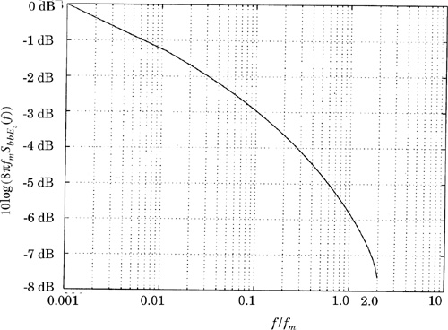
The spectral shape of the Doppler spread determines the time domain fading waveform and dictates the temporal correlation and fade slope behaviors. Rayleigh fading simulators must use a fading spectrum such as Equation (5.78) in order to produce realistic fading waveforms that have proper time correlation.
It is often useful to simulate multipath fading channels in hardware or software. A popular simulation method uses the concept of in-phase and quadrature modulation paths to produce a simulated signal representing Equation (5.63) with spectral and temporal characteristics very close to measured data.
As shown in Figure 5.22(b), two independent Gaussian low pass noise sources are used to produce in-phase and quadrature fading branches. Each Gaussian source may be formed by summing two independent Gaussian random variables which are orthogonal (i.e., g = a + jb, where a and b are real Gaussian random variables and g is complex Gaussian). By using the spectral filter defined by Equation (5.78) to shape the random signals in the frequency domain, accurate time domain waveforms of Doppler fading can be produced by using an inverse fast Fourier transform (IFFT) at the last stage of the simulator.

Smith [Smi75] demonstrated a simple computer program that implements Figure 5.22(b). His method uses a complex Gaussian random number generator (noise source) to produce a baseband line spectrum with complex weights in the positive frequency band. The maximum frequency component of the line spectrum is fm. Using the property of real signals, the negative frequency components are constructed by simply conjugating the complex Gaussian values obtained for the positive frequencies. Note that the IFFT of each complex Gaussian signal should be a purely real Gaussian random process in the time domain which is used in each of the quadrature arms shown in Figure 5.24. The random valued line spectrum is then multiplied with a discrete frequency representation of ![]() having the same number of points as the noise source. To handle the case where Equation (5.78) approaches infinity at the passband edge, Smith truncated the value of SEz (fm) by computing the slope of the function at the sample frequency just prior to the passband edge and increasing the slope to the passband edge. Simulations using the architecture in Figure 5.22 are usually implemented in the frequency domain using complex Gaussian line spectra to take advantage of easy implementation of Equation (5.78). This, in turn, implies that the low pass Gaussian noise components are actually a series of frequency components (line spectrum from −fm to fm), which are equally spaced and each have a complex Gaussian weight. Smith’s simulation methodology is shown in Figure 5.24.
having the same number of points as the noise source. To handle the case where Equation (5.78) approaches infinity at the passband edge, Smith truncated the value of SEz (fm) by computing the slope of the function at the sample frequency just prior to the passband edge and increasing the slope to the passband edge. Simulations using the architecture in Figure 5.22 are usually implemented in the frequency domain using complex Gaussian line spectra to take advantage of easy implementation of Equation (5.78). This, in turn, implies that the low pass Gaussian noise components are actually a series of frequency components (line spectrum from −fm to fm), which are equally spaced and each have a complex Gaussian weight. Smith’s simulation methodology is shown in Figure 5.24.


To implement the simulator shown in Figure 5.24, the following steps are used:
Specify the number of frequency domain points (N) used to represent
 and the maximum Doppler frequency shift (fm). The value used for N is usually a power of two.
Compute the frequency spacing between adjacent spectral lines as Δf = 2fm/(N − 1). This defines the time duration of a fading waveform, T = 1/Δf.
Generate complex Gaussian random variables for each of the N/2 positive frequency components of the noise source.
Construct the negative frequency components of the noise source by conjugating positive frequency values and assigning these at negative frequency values.
Multiply the in-phase and quadrature noise sources by the fading spectrum
.Perform an IFFT on the resulting frequency domain signals from the in-phase and quadrature arms to get two N-length time series, and add the squares of each signal point in time to create an N-point time series like under the radical of Equation (5.67). Note that each quadrature arm should be a real signal after the IFFT to model Equation (5.63).
Take the square root of the sum obtained in Step 6 to obtain an N-point time series of a simulated Rayleigh fading signal with the proper Doppler spread and time correlation.
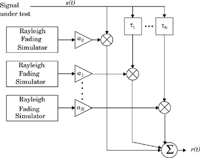
Several Rayleigh fading simulators may be used in conjunction with variable gains and time delays to produce frequency selective fading effects. This is shown in Figure 5.25.
By making a single frequency component dominant in amplitude within ![]() and at f = 0, the fading is changed from Rayleigh to Ricean. For a multipath fading simulator with many resolvable components, this mtheod can be used to alter the probability distributions of the individual multipath components in the simulator of Figure 5.25. One must take care to properly implement the IFFT such that each arm of Figure 5.24 produces a real time domain signal as given by Tc(t) and Ts(t) in Equations (5.64) and (5.65).
and at f = 0, the fading is changed from Rayleigh to Ricean. For a multipath fading simulator with many resolvable components, this mtheod can be used to alter the probability distributions of the individual multipath components in the simulator of Figure 5.25. One must take care to properly implement the IFFT such that each arm of Figure 5.24 produces a real time domain signal as given by Tc(t) and Ts(t) in Equations (5.64) and (5.65).
To determine the impact of flat fading on an applied signal s(t), one merely needs to multiply the applied signal by r(t), the output of the fading simulator. To determine the impact of more than one multipath component, a convolution must be performed as shown in Figure 5.25.
Rice computed joint statistics for a mathematical problem which is similar to Clarke’s fading model [Cla68], and thereby provided simple expressions for computing the average number of level crossing and the duration of fades. The level crossing rate (LCR) and average fade duration of a Rayleigh fading signal are two important statistics which are useful for designing error control codes and diversity schemes to be used in mobile communication systems, since it becomes possible to relate the time rate of change of the received signal to the signal level and velocity of the mobile.
The level crossing rate (LCR) is defined as the expected rate at which the Rayleigh fading envelope, normalized to the local rms signal level, crosses a specified level in a positive-going direction. The number of level crossings per second is given by

where ![]() is the time derivative of r(t) (i.e., the slope), p(R,
is the time derivative of r(t) (i.e., the slope), p(R,![]() ) is the joint density function of r and
) is the joint density function of r and ![]() at r = R, fm is the maximum Doppler frequency, and ρ = R/Rrms is the value of the specified level R, normalized to the local rms amplitude of the fading envelope [Jak74]. Equation (5.80) gives the value of NR, the average number of level crossings per second at specified R. The level crossing rate is a function of the mobile speed as is apparent from the presence of fm in Equation (5.80). There are few crossings at both high and low levels, with the maximum rate occurring at
at r = R, fm is the maximum Doppler frequency, and ρ = R/Rrms is the value of the specified level R, normalized to the local rms amplitude of the fading envelope [Jak74]. Equation (5.80) gives the value of NR, the average number of level crossings per second at specified R. The level crossing rate is a function of the mobile speed as is apparent from the presence of fm in Equation (5.80). There are few crossings at both high and low levels, with the maximum rate occurring at ![]() , (i.e., at a level 3 dB below the rms level). The signal envelope experiences very deep fades only occasionally, but shallow fades are frequent.
, (i.e., at a level 3 dB below the rms level). The signal envelope experiences very deep fades only occasionally, but shallow fades are frequent.
Example 5.7.
For a Rayleigh fading signal, compute the positive-going level crossing rate for ρ = 1, when the maximum Doppler frequency (fm) is 20 Hz. What is the maximum velocity of the mobile for this Doppler frequency if the carrier frequency is 900 MHz?
Solution
Using Equation (5.80), the number of zero level crossings is
The maximum velocity of the mobile can be obtained using the Doppler relation, fd, max = v/λ.
Therefore velocity of the mobile at fm = 20 Hz is
v = fdλ = 20 Hz(1/3 m) = 6.66 m/s = 24 km/hr |
The average fade duration is defined as the average period of time for which the received signal is below a specified level R. For a Rayleigh fading signal, this is given by
where Pr[r≤R] is the probability that the received signal r is less than R and is given by
where τi is the duration of the fade and T is the observation interval of the fading signal. The probability that the received signal r is less than the threshold R is found from the Rayleigh distribution as
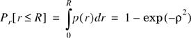
where p(r) is the pdf of a Rayleigh distribution. Thus, using Equations (5.80), (5.81), and (5.83), the average fade duration as a function of ρ and fm can be expressed as

The average duration of a signal fade helps determine the most likely number of signaling bits that may be lost during a fade. Average fade duration primarily depends upon the speed of the mobile, and decreases as the maximum Doppler frequency fm becomes large. If there is a particular fade margin built into the mobile communication system, it is appropriate to evaluate the receiver performance by determining the rate at which the input signal falls below a given level R, and how long it remains below the level, on average. This is useful for relating SNR during a fade to the instantaneous BER which results.
Example 5.8.
Find the average fade duration for threshold levels ρ = 0.01, ρ = 0.1, and ρ = 1, when the Doppler frequency is 200 Hz.
Solution
Average fade duration can be found by substituting the given values in Equation (5.84)
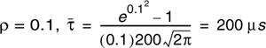

Example 5.9.
Find the average fade duration for a threshold level of ρ = 0.707 when the Doppler frequency is 20 Hz. For a binary digital modulation with bit duration of 50 bps, is the Rayleigh fading slow or fast? What is the average number of bit errors per second for the given data rate. Assume that a bit error occurs whenever any portion of a bit encounters a fade for which ρ < 0.1.
Solution
The average fade duration can be obtained using Equation (5.84).
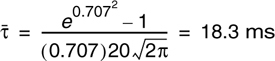
For a data rate of 50 bps, the bit period is 20 ms. Since the bit period is greater than the average fade duration, for the given data rate the signal undergoes fast Rayleigh fading. Using Equation (5.84), the average fade duration for ρ = 0.1 is equal to 0.002 s. This is less than the duration of one bit. Therefore, only one bit on average will be lost during a fade. Using Equation (5.80), the number of level crossings for ρ = 0.1 is Nr = 4.96 crossings per seconds. Since a bit error is assumed to occur whenever a portion of a bit encounters a fade, and since average fade duration spans only a fraction of a bit duration, the total number of bits in error is 5 per second, resulting in a BER = (5/50) = 0.1.
Clarke’s model and the statistics for Rayleigh fading are for flat fading conditions and do not consider multipath time delay. In modern mobile communication systems with high data rates, it has become necessary to model the effects of multipath delay spread as well as fading. A commonly used multipath model is an independent Rayleigh fading two-ray model (which is a specific implementation of the generic fading simulator shown in Figure 5.25). Figure 5.26 shows a block diagram of the two-ray independent Rayleigh fading channel model. The impulse response of the model is represented as
where α1 and α2 are independent and Rayleigh distributed, ф1 and ф2 are independent and uniformly distributed over [0, 2π], and τ is the time delay between the two rays. By setting α2 equal to zero, the special case of a flat Rayleigh fading channel is obtained as
By varying τ, it is possible to create a wide range of frequency selective fading effects. The proper time correlation properties of the Rayleigh random variables α1 and α2 are guaranteed by generating two independent waveforms, each produced from the inverse Fourier transform of the spectrum described in Section 5.7.2.
Saleh and Valenzuela [Sal87] reported the results of indoor propagation measurements between two vertically polarized omnidirectional antennas located on the same floor of a medium sized office building. Measurements were made using 10 ns, 1.5 GHz, radar-like pulses. The method involved averaging the square law detected pulse response while sweeping the frequency of the transmitted pulse. Using this method, multipath components within 5 ns were resolvable.
The results obtained by Saleh and Valenzuela show that: (a) the indoor channel is quasistatic or very slowly time varying, and (b) the statistics of the channel impulse response are independent of transmitting and receiving antenna polarization, if there is no line-of-sight path between them. They reported a maximum multipath delay spread of 100 ns to 200 ns within the rooms of a building, and 300 ns in hallways. The measured rms delay spread within rooms had a median of 25 ns and a maximum of 50 ns. The large-scale path loss with no line-of-sight path was found to vary over a 60 dB range and obey a log-distance power law (see Equation (4.68)) with an exponent between three and four.
Saleh and Valenzuela developed a simple multipath model for indoor channels based on measurement results. The model assumes that the multipath components arrive in clusters. The amplitudes of the received components are independent Rayleigh random variables with variances that decay exponentially with cluster delay as well as excess delay within a cluster. The corresponding phase angles are independent uniform random variables over [0, 2π]. The clusters and multipath components within a cluster form Poisson arrival processes with different rates. The clusters and multipath components within a cluster have exponentially distributed interarrival times. The formation of the clusters is related to the building structure, while the components within the cluster are formed by multiple reflections from objects in the vicinity of the transmitter and the receiver.
Rappaport and Seidel [Rap91a] reported measurements at 1300 MHz in five factory buildings and carried out subsequent measurements in other types of buildings. The authors developed an elaborate, empirically derived statistical model to generate measured channels based on the discrete impulse response channel model of Equation (5.12) and wrote a computer program called SIRCIM (Simulation of Indoor Radio Channel Impulse-response Models). SIRCIM generates realistic samples of small-scale indoor channel impulse response measurements [Rap91a]. Subsequent work by Huang produced SMRCIM (Simulation of Mobile Radio Channel Impulse-response Models), a similar program that generates small-scale urban cellular and microcellular channel impulse responses [Rap93a]. These programs are currently in use at over 100 institutions throughout the world, and have been updated to include angle of arrival information for microcell, indoor, and macrocell channels [Nuc99], [Lib99].
By recording power delay profile impulse responses at λ/4 intervals on a 1 m track at many indoor measurement locations, the authors were able to characterize local small-scale fading of individual multipath components, and the small-scale variation in the number and arrival times of multipath components within a local area. Thus, the resulting statistical models are functions of multipath time delay bin τi, the small-scale receiver spacing, Xl, within a 1 m local area, the topography Sm which is either line-of-sight (LOS) or obstructed, the large-scale T–R separation distance Dn, and the particular measurement location Pn. Therefore, each individual baseband power delay profile is expressed in a manner similar to Equation (5.12), except the random amplitudes and time delays are random variables which depend on the surrounding environment. Phases are synthesized using a pseudo-deterministic model which provides realistic results, so that a complete time varying complex baseband channel impulse response hb (t;τi) may be obtained over a local area through simulation.

In Equation (5.87), ![]() is the average multipath receiver power within a discrete excess delay interval of 7.8125 ns.
is the average multipath receiver power within a discrete excess delay interval of 7.8125 ns.
The measured multipath delays inside open-plan buildings ranged from 40 ns to 800 ns. Mean multipath delay and rms delay spread values ranged from 30 ns to 300 ns, with median values of 96 ns in LOS paths and 105 ns in obstructed paths. Delay spreads were found to be uncorrelated with T–R separation but were affected by factory inventory, building construction materials, building age, wall locations, and ceiling heights. Measurements in a food processing factory that manufactures dry-goods and has considerably less metal inventory than other factories had an rms delay spread that was half of those observed in factories producing metal products. Newer factories which incorporate steel beams and steel reinforced concrete in the building structure have stronger multipath signals and less attenuation than older factories which used wood and brick for perimeter walls. The data suggested that radio propagation in buildings may be described by a hybrid geometric/statistical model that accounts for both reflections from walls and ceilings and random scattering from inventory and equipment.
By analyzing the measurements from fifty local areas in many buildings, it was found that the number of multipath components, Np, arriving at a certain location is a function of X, Sm, and Pn, and almost always has a Gaussian distribution. The average number of multipath components ranges between 9 and 36, and is generated based on an empirical fit to measurements. The probability that a multipath component will arrive at a receiver at a particular excess delay Ti in a particular environment Sm is denoted as PR(Ti,Sm). This was found from measurements by counting the total number of detected multipath components at a particular discrete excess delay time, and dividing by the total number of possible multipath components for each excess delay interval. The probabilities for multipath arriving at a particular excess delay values may be modeled as piecewise functions of excess delay, and are given by

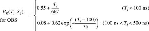
where S1 corresponds to the LOS topography, and S2 corresponds to obstructed topography. SIRCIM uses the probability of arrival distributions described by Equation (5.88) or (5.89) along with the probability distribution of the number of multipath components, Np(X, Sm,Pn), to simulate power delay profiles over small-scale distances. A recursive algorithm repeatedly compares Equation (5.88) or (5.89) with a uniformly distributed random variable until the proper NP is generated for each profile [Hua91], [Rap91a].
Figure 5.27 shows an example of measured power delay profiles at 19 discrete receiver locations along a 1 m track, and illustrates accompanying narrowband information which SIRCIM computes based on synthesized phases for each multipath component [Rap91a]. Measurements reported in the literature provide excellent agreement with impulse responses predicted by SIRCIM.
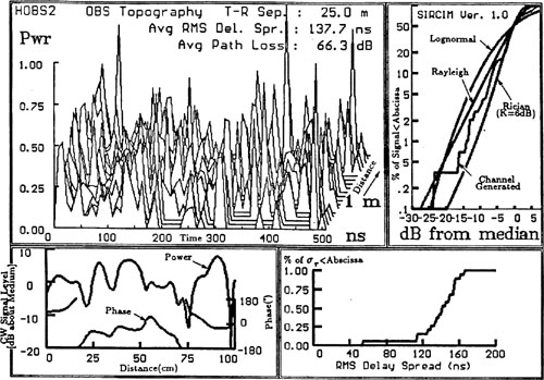
Figure 5.27. Indoor wideband impulse responses simulated by SIRCIM at 1.3 GHz. Also shown are the distributions of the rms delay spread and the narrowband signal power distribution. The channel is simulated as being obstructed in an open-plan building, T–R separation is 25 m. The rms delay spread is 137.7 ns. All multipath components and parameters are stored on disk.
Using similar statistical modeling techniques, urban cellular and microcellular multipath measurement data from [Rap90], [Sei91], [Sei92a] were used to develop SMRCIM. Both large cell and microcell models were developed. Figure 5.28 shows an example of SMRCIM output for an outdoor microcell environment [Rap93a].
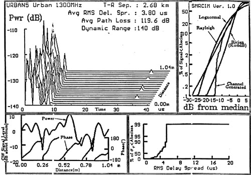
A new method of analysis has been developed that characterizes the flat, small-scale fading experienced by a receiver in an arbitrary spatial-temporal channel [Dur00]. This method characterizes a multipath channel with arbitrary spatial complexity to three shape factors that have simple, intuitive geometrical interpretations. Furthermore, these shape factors describe the statistics of received signal fluctuations in a fading multipath channel. Analytical expressions for level-crossing rate, average fade duration, envelope autocovariance, and coherence distance are easily derived using the new shape factor theory, and match all of the classical results in [Jak74].
The term small-scale fading describes the rapid fluctuations of received power level due to small, sub-wavelength changes in receiver position. This effect is due to the constructive and destructive interference of the numerous multipath waves that impinge upon a wireless receiver [Jak74]. The resulting signal strength fluctuations affect, in some way, nearly every aspect of receiver design: dynamic range, equalization, diversity, modulation scheme, and channel and error-correction coding. These fluctuations are a function of direction of travel as related to the angle of arrival of multipath delay.
Numerous researchers have measured and analyzed the first-order statistics of these processes, which mostly involves the characterization of small-scale fading with a probability density function (PDF) discussed in Section 5.6 [Ric48], [Suz77], [Cou98]. The autocorrelation statistics of fading processes, or second-order statistics, include measures of a process such as power spectral density (PSD), level-crossing rate, and average fade duration, as discussed in Section 5.7
It turns out that second-order statistics are heavily dependent on the angles-of-arrival of received multipath, yet they have traditionally been studied using an omnidirectional, azimuthal propagation model as shown in Section 5.7 [Jak74]. That is, multipath waves usually are assumed to arrive at the receiver with equal power from the horizon in every possible direction. Truthfully, no realistic channel resembles this idealized model, but it is a reasonable multipath propagation model for receivers operating in heavily shadowed regions with a dense concentration of scatterers, and yields analytical results which resembled early field measurements [Cla68]. Clarke’s model conveniently produces analytical statistics that are isotropic, unrealistically identical regardless of the direction traveled by the mobile receiver. Unfortunately, recent measurements and models have shown that the arriving multipath in a local area bears little resemblance to the omnidirectional propagation assumption and, in fact, the direction of travel relative to the arriving multipath is a key factor in producing the observed fading [Ros97], [Fuh97]. An approximately omnidirectional channel model does not accurately describe fading statistics if directional or smart antenna systems are employed at a receiver [Win98, Lib99, Mol01].
The new concept of multipath shape factors allows the quantitative analysis of any distribution of non-omnidirectional multipath waves in a local area (where the local average signal strength is assumed to be wide-sense stationary). Three principle shape factors—the angular spread, the angular constriction, and the azimuthal direction of maximum fading—are defined and exactly related to the average rate at which a received signal fades [Dur99]. Four of the basic second-order small-scale fading statistics—level-crossing rate, average fade duration, autocovariance, and coherence distance—may be described in terms of this multipath shape factor theory. As shown subsequently, several classical propagation problems are analyzed easily using multipath shape factors.
Three multipath shape factors influence second-order fading statistics, and these may be derived from the angular distribution of multipath power, p(θ), which is a general representation of from-the-horizon propagation in a local area [Gan72]. This representation of p(θ) includes antenna gains and polarization mismatch effects [Dur98a]. The shape factors are based on the complex Fourier coefficients of p(θ):

where Fn is the nth complex Fourier coefficient. The utility of these three shape factors becomes clear in Section 5.8.1.2.
The shape factor angular spread, Λ, is a measure of how multipath concentrates about a single azimuthal direction of arrival. We define angular spread to be
where F0 and F1 are defined by Equation (5.90). There are several advantages to defining angular spread by Equation (5.91). First, since angular spread is normalized by F0 (the total amount of local average received power), it is invariant under changes in transmitted power. Second, Λ is invariant under any series of rotational or reflective transformations of p(θ). Finally, this definition is intuitive; angular spread ranges from 0 to 1, whereby 0 denotes the extreme case of a single multipath component from a single direction and 1 denotes no clear bias in the angular distribution of received power (e.g., Clarke’s model).
It should be noted that other definitions exist in the literature for angular spread. These definitions involve either beamwidth or the RMS θ calculations and are often ill-suited for general application to arbitrary channels or periodic functions such as p(θ) [Ebi91], [Nag96], [Ful98], [Jen98].
The shape factor angular constriction, γ, is a measure of how multipath concentrates about two azimuthal directions. We define angular constriction to be
where F0, F1, and F2 are defined by Equation (5.90). Much like the definition of angular spread, the measure for angular constriction is invariant under changes in transmitted power or any series of rotational or reflective transformations of p(θ). The possible values of angular constriction, γ, range from 0 to 1, with 0 denoting no clear bias in two arrival directions and 1 denoting the extreme case of exactly two multipath components arriving from different directions.
A third shape factor, which may be thought of as a directional, or orientation, parameter, is the azimuthal direction of maximum fading, θmax. We define this parameter to be
The θmax value corresponds to the direction in which a mobile user would move in order to experience the maximum fading rate in the local area.
Complex received voltage, received power, and received envelope are the three basic stochastic processes that are studied in small-scale fading. In order to understand how these stochastic processes evolve over space, it is useful to study the position derivatives or rate-of-changes of the three processes. Since the mean derivative of a stationary process is zero, the mean-squared derivative is the simplest statistic that measures the fading rate of a channel. In fact, a mean-squared derivative of a stationary process is actually the variance of the rate-of-change. This section, therefore, presents equations for describing the rate variance relationships of small-scale received complex voltage, power, and envelope fluctuations. All of these relationships are proven exactly in Appendix C.
The complex received voltage, ![]() , is a baseband representation of the summation of numerous multipath waves that have impinged upon the receiver antenna and have excited a complex voltage component at the input of a receiver (see Section 5.2). Appendix C.1 derives the rate variance,
, is a baseband representation of the summation of numerous multipath waves that have impinged upon the receiver antenna and have excited a complex voltage component at the input of a receiver (see Section 5.2). Appendix C.1 derives the rate variance, ![]() , for the complex voltage of a receiver traveling along the azimuthal direction θ:
, for the complex voltage of a receiver traveling along the azimuthal direction θ:
where λ is the wavelength of the carrier frequency, PT is the local average mean-squared received power (units of volts-squared). Note that the dependence on multipath angle-of-arrival in Equation (5.94) may be reduced to the three basic shape factors: angular spread, angular constriction, and the azimuthal direction of maximum fading. The physical significance of ![]() is that it describes the spatial selectivity of a channel in a local area and, by extension, the average complex voltage fluctuations for a mobile receiver as it moves over a local area.
is that it describes the spatial selectivity of a channel in a local area and, by extension, the average complex voltage fluctuations for a mobile receiver as it moves over a local area.
Received power, Pr, is equal to the magnitude-squared of complex voltage, ![]() . Note that this definition of power yields units of volts-squared rather than watts, which would differ only by a constant of proportionality related to the input impedance of the receiver; the volts-squared definition is more general and independent of the receiver used.
. Note that this definition of power yields units of volts-squared rather than watts, which would differ only by a constant of proportionality related to the input impedance of the receiver; the volts-squared definition is more general and independent of the receiver used.
The mathematical operation of taking the squared magnitude of a complex quantity is a nonlinear operation, so in order to derive a rate variance relationship for received power, we will assume that the channel is Rayleigh fading. This assumption, however, is unnecessary for the derivation of Equation (5.94). Appendix C.2 derives the rate variance, ![]() , for the power of a receiver traveling along the azimuthal direction θ:
, for the power of a receiver traveling along the azimuthal direction θ:
Once again, the dependence on multipath angle-of-arrival in Equation (5.95) may be reduced entirely to the three basic shape factors. The physical significance of ![]() is that it describes the average received power fluctuations in a local area where the signal envelope undergoes Rayleigh flat fading.
is that it describes the average received power fluctuations in a local area where the signal envelope undergoes Rayleigh flat fading.
Received envelope, R(r), is equal to the magnitude of complex voltage, ![]() . Once again, we assume that the channel is Rayleigh fading to calculate the mean-squared fading rate. Appendix C.3 shows how this assumption leads to the envelope rate variance,
. Once again, we assume that the channel is Rayleigh fading to calculate the mean-squared fading rate. Appendix C.3 shows how this assumption leads to the envelope rate variance,
Again, Equation (5.96) depends on Λ, γ, and θmax. The physical significance of ![]() is that it describes the average envelope fluctuations in a local area where the signal envelope undergoes Rayleigh flat fading.
is that it describes the average envelope fluctuations in a local area where the signal envelope undergoes Rayleigh flat fading.
Applying the three shape factors, Λ, γ, and θmax, to the classical omnidirectional propagation model of Section 5.7, we find that there is not a bias in either one or two directions of angle-of-arrival, leading to maximum angular spread (Λ = 1) and minimum angular constriction (γ = 0). The statistics of omnidirectional propagation are isotropic, exhibiting no dependence on the azimuthal direction of receiver travel, θ.
If the rate variance relationships of Equations (5.94)–(5.96) are normalized against their values for omnidirectional propagation, then they reduce to the following form:

where ![]() is a normalized fading rate variance. Equation (5.97) provides a convenient way to analyze the effects of the shape factors on the second-order statistics of small-scale fading.
is a normalized fading rate variance. Equation (5.97) provides a convenient way to analyze the effects of the shape factors on the second-order statistics of small-scale fading.
First, notice that angular spread, Λ, describes the average fading rate within a local area. A convenient way of viewing this effect is to consider the fading rate variance taken along two perpendicular directions within the same local area. From Equation (5.97), the average of the two fading rate variances, regardless of the orientation of the measurement, is always given by averaging the variances observed over two perpendicular directions within the local area
Equation (5.98) clearly shows that the average fading rate within a local area decreases with respect to omnidirectional propagation as multipath power becomes more and more concentrated about a single azimuthal direction. A method for measuring multipath angular spread based on this relationship has been presented in [Pat99].
Second, notice that angular constriction, γ, does not affect the average fading rate within a local area, but describes the variability of fading rates taken along different azimuthal directions, θ. From Equation (5.97), fading rate variance ![]() will change as a function of direction of receiver travel θ, but will always fall within the following range:
will change as a function of direction of receiver travel θ, but will always fall within the following range:
The upper limit of Equation (5.99) corresponds to a receiver traveling in the azimuthal direction of maximum fading (θ = θmax) while the lower limit corresponds to travel in a perpendicular direction (θ = θmax + π/2). Equation (5.99) clearly shows that the variability of fading rates within the same local area increases as the channel becomes more and more constricted.
It is interesting to note that the propagation mechanisms of a channel are not uniquely described by the three shape factors Λ, γ, and θmax. An infinitum of propagation mechanisms exist which may have the same set of shape factors and, by extension, lead to channels which exhibit nearly the same end-to-end performance. In fact, Equation (5.97) provides rigorous mathematical criteria for a multipath channel that may be treated as “pseudo-omnidirectional”:
Under the condition of Equation (5.100), angular spread becomes approximately 1 and angular constriction becomes approximately 0. Thus, the second-order statistics of the channel behave nearly identical to the classical omnidirectional channel developed by Clarke and Gans.
This section presents four different analytical examples of non-omnidirectional propagation channels that provide insight into the shape factor definitions and how they describe fading rates.
Consider the simplest small-scale fading situation where two coherent, constant-amplitude multipath components, with individual powers defined by P1 and P2, arrive at a mobile receiver separated by an azimuthal angle α. We call this the two-wave channel model. Figure 5.29 illustrates this angular distribution of power, which is mathematically defined as
where θo is an arbitrary offset angle and δ(·) is an impulse function. By applying Equations (5.91)–(5.93), the expressions for Λ, γ, and θmax for this distribution are
The angular constriction, γ, is always 1 because the two-wave model represents perfect clustering about two directions. The limiting case of two multipath components arriving from the same direction (α = 0) results in an angular spread, Λ, of 0. An angular spread of 1 results only when two multipath of identical powers (P1 = P2) are separated by α = 180°. Figure 5.29 shows how the fading behavior changes as multipath separation angle, α, increases for the case of two equal-powered waves. Thus, increasing α changes a channel with low spatial selectivity into a channel with high spatial selectivity that exhibits a strong dependence on the azimuthal direction of receiver motion.
Consider another theoretical situation where multipath power is arriving continuously and uniformly over a range of azimuth angles. This model has been used to describe propagation for directional receiver antennas with a distinct azimuthal beam [Gan72]. The function p(θ) will be defined by
The angle α indicates the width of the sector (in radians) of arriving multipath power and the angle θo is an arbitrary offset angle, as illustrated by Figure 5.30. By applying Equations (5.91)–(5.93), the expressions for Λ, γ, and θmax for this distribution are

The limiting cases of these parameters and Equation (5.95) provide deeper understanding of angular spread and constriction.
Figure 5.30 graphs the spatial channel parameters, Λ and γ, as a function of sector width, α. The limiting case of a single multipath arriving from precisely one direction corresponds to α = 0, which results in the minimum angular spread of Λ = 0. The other limiting case of uniform illumination in all directions corresponds to α = 360° (omnidirectional Clarke model), which results in the maximum angular spread of Λ = 1. The angular constriction, γ, follows an opposite trend. It is at a maximum (γ = 1) when α = 0 and at a minimum (γ = 0) when α = 360°. The graph in Figure 5.30 shows that as the multipath angles of arrival are condensed into a smaller and smaller sector, the directional dependence of fading rates within the same local area increases. Overall, however, fading rates decrease with decreasing sector size α.
Another example of angular constriction may be studied using the Double Sector model of Figure 5.31. Diffuse multipath propagation over two equal and opposite sectors of azimuthal angles characterize the incoming power. The equation that describes this angular distribution of power is


The angle α is the sector width and the angle θo is an arbitrary offset angle. By applying Equations (5.91)–(5.93), the expressions for Λ, γ, and θmax for this distribution are
Note that the value of angular spread, Λ, is always 1. Regardless of the value of α, an equal amount of power arrives from opposite directions, producing no clear bias in the direction of multipath arrival.
The limiting case of α = 180° (omnidirectional propagation) results in an angular constriction of γ = 0. As α decreases, the angular distribution of power becomes more and more constricted. In the limit of α = 0, the value of angular constriction reaches its maximum, γ = 1. This case corresponds to the above-mentioned instance of two-wave propagation. Figure 5.31 shows how the fading behavior changes as sector width α increases, making the fading rate more and more isotropic while the RMS average remains constant.
A Ricean channel model results from the addition of a single plane wave and numerous diffusely scattered waves [Ric48]. If the power of the scattered waves is assumed to be evenly distributed in azimuth, then the channel may be modeled by the following p(θ):
where K is the ratio of coherent to diffuse incoherent power, often referred to as the Ricean K-factor. By applying Equations (5.91)–(5.93), the expressions for Λ, γ, and θmax for this distribution are
Figure 5.32 depicts the spatial channel parameters, Λ and γ, as a function of K-factor. For very small K-factors, the channel appears to be omnidirectional (Λ = 1 and γ = 0). As the K-factor increases, the angular spread of the Ricean channel decreases and the angular constriction increases. This indicates that the overall fading rate in the Ricean channel decreases and that the differences between the minimum and maximum fading rate variances within the same local area but different directions increases.

Second-Order Statistics Using Shape Factors [Dur00]
With an understanding of how shape factors describe fading rate variances, it is possible to re-derive many of the basic second-order statistical measures of fading channels given in Section 5.7.3 in terms of the three shape factors. Level-crossing rates, average fade duration, spatial autocovariance, and coherence distance expressions that were originally derived under the assumption of omnidirectional multipath propagation will now be cast in terms of the angular spread, the angular constriction, and the azimuthal direction of maximum fading [Dur99], [Dur99a], [Dur99b].
The derivations focus on Rayleigh channels, since these types of channels are analytically tractable. A Rayleigh fading signal is one whose envelope, R, follows a Rayleigh PDF, pR(r), given by Equation (5.49) which can be expressed as
where PT is the average total power received in a local area (units of volts-squared).
The general expression for a level-crossing rate is given by (5.80) [Jak74]:
where R is the threshold level and p(R,![]() ) is the joint PDF of envelope and its time derivative. For a Rayleigh-fading signal, the level-crossing rate of the envelope process is
) is the joint PDF of envelope and its time derivative. For a Rayleigh-fading signal, the level-crossing rate of the envelope process is

The variable ρ is the normalized threshold level, such that ρ = R2/PT [Jak74]. Note that ![]() is simply the time-derivative equivalent of
is simply the time-derivative equivalent of ![]() , derived in Appendix C.1, which arises from a mobile receiver traveling through space with a constant velocity in an otherwise static channel (transmitter and scatterers are fixed).
, derived in Appendix C.1, which arises from a mobile receiver traveling through space with a constant velocity in an otherwise static channel (transmitter and scatterers are fixed).
By substituting Equation (5.94) into Equation (5.111), we arrive at an exact expression for the level-crossing rate in a Rayleigh fading channel with any arbitrary spatial distribution of multipath power and any direction of mobile receiver travel, θ:
The average fade duration, ![]() , is defined to be [Jak74], [Cla68]
, is defined to be [Jak74], [Cla68]

Substitution of the Rayleigh PDF of Equations (5.109) and (5.112) into Equation (5.113) yields

Equations (5.112) and (5.114) are useful tools for studying small-scale fading statistics in the presence of non-omnidirectional multipath, and yield identical results to those given in Section 5.7.3 when an omnidirectional channel is assumed.
Another important second-order statistic is the spatial autocovariance of received voltage envelope. The autocovariance function determines the correlation of received voltage envelope as a function of change in receiver position and is useful for studies in spatial diversity [Jak74], [Vau93]. Appendix D develops an approximate expression for the spatial autocovariance function of envelope based on shape factors [Dur99a]. The approximation is given by
Equation (5.115) allows us to estimate the envelope correlation between two points in space separated by a distance r along an azimuthal direction θ. The behavior of Equation (5.115) is benchmarked in Section 5.8.5 against several known analytical solutions presented in [Jak74].
Coherence distance, Dc, is the separation distance in space over which a fading channel appears to be unchanged. As shown in Chapter 7, coherence distance is important in the design of wireless receivers that employ spatial diversity to combat spatial selectivity. For mobile receivers, a similar parameter called coherence time, Tc, is the elapsed time over which a fading channel appears to be constant (see Equation (5.40.b)). For the case of a static channel, the coherence time of a mobile receiver may be calculated from the coherence distance (Tc = Dc/v, where v is the speed of the mobile).
Definitions for coherence distance may be based on the envelope autocovariance function. A convenient definition for the coherence distance, Dc, is the value that satisfies the equation ρ(Dc) = 0.5 [Ste94]. The classical value for coherence distance in an omnidirectional Rayleigh channel is given by
Using the generalized autocovariance function of Equation (5.115) leads to a new definition of coherence distance:
For omnidirectional propagation, Equation (5.117) differs from Equation (5.116) by only –3.0%. Furthermore, Equation (5.117) captures the behavior of non-omnidirectional multipath. As angular spread, Λ, decreases, the coherence distance in a local area increases. As the angular constriction, γ, increases, the coherence distance develops a strong dependence on orientation, θ.
The theory presented in Section 5.8 was originally developed for a flat fading small scale assumption. By realizing that wideband channels may be modeled as discrete, resolvable multipath components in time delay, one can readily see how the theory may be applied to each resolvable time delay bin, as shown in Figure 5.4. The shape factor theory allows the fading statistics of individual multipath to be studied [Pat99].
As a point of comparison, we now analyze three well-known cases of propagation that have analytical solutions as described in Sections 5.7.1–5.7.3 [Jak74]. The cases are analyzed using the shape factor approach as outlined in Section 5.7.4 for mobile receivers with speed v. This approach is shown to produce quick, comprehensive, and—most importantly—accurate solutions.
The first case corresponds to a narrowband receiver operating in a local area with multipath arriving from all directions, such that the angular distribution of power, p(θ), is a constant. The receiver antenna is assumed to be an omnidirectional whip, oriented perpendicular to the ground. Due to the vertical electric-field polarization of the whip antenna, this propagation scenario is referred to as the Ez-case [Cla68].
The second two cases correspond to the same narrowband receiver in the same omnidirectional multipath channel, but with a small loop antenna mounted atop the receiver such that the plane of the loop is perpendicular to the ground. The antenna pattern of the small loop antenna attenuates the arriving multipath such that the angular distribution of power becomes
where A is some arbitrary gain constant. Unlike the omnidirectional Ez-case, the statistics of this propagation scenario will depend on the direction of travel by the receiver. The Hx-case will refer to a receiver traveling in a direction perpendicular to the main lobes of the loop antenna pattern (θ = 0). The Hy-case will refer to a receiver traveling in a direction parallel to the main lobes (θ = π/2). Figure 5.33 illustrates the Ez, Hx, and Hy cases for the modeled receiver antennas.

The first step is to calculate the three spatial parameters from the angular distribution of power, p(θ), using Equations (5.91)–(5.93). The spatial parameters for the Ez-case are Λ, γ, and θmax = 0. Since this case is omnidirectional, the angular spread is at a maximum (Λ = 1) and the angular constriction is at a minimum (γ = 0). For the Hx- and Hy-cases, the spatial parameters are Λ = 1, γ = 1/2, and θmax = π/2. Since the impinging multipath have no clear bias in one direction, the angular spread is at a maximum just like the Ez-case. However, there is clearly a bias in two directions, resulting in an increased angular constriction of γ = 1/2.
After substitution of these parameters into Equation (5.112) along with the appropriate direction of mobile travel, the level-crossing rates for the three cases become
The corresponding average fade durations are


These expressions exactly match the original solutions presented by Clarke in [Cla68].
Now substitute the channel shape factors into the approximate spatial autocovariance functions in Equation (5.115). The results for the three cases are
These three functions are compared to their more rigorous analytical solutions in Figure 5.34 through Figure 5.36. Note that all three model the spatial autocovariance function consistent with the approximation made in the derivation of Equation (5.115). The behavior is nearly exact for values of r equal to or less than a correlation distance.

The shape factor technique for finding fading statistics is an intuitive way to relate the physical channel characteristics to the fading behavior. In the previous examples, the spatial parameters may be calculated analytically or even estimated intuitively by simply looking at the distributions of multipath power in Figure 5.33. The use of spatial parameters to find level crossing rate, average fade duration, and spatial autocovariance is quite simple when compared to the full analytical solutions of the Ez, Hx, and Hy-cases presented in [Jak74]. The proposed solution is also more comprehensive. For example, once the shape factors have been found, Equations (5.112), (5.114), and (5.115) provide statistics for all directions of travel for the Hx- and Hy-cases, and not just specific directions such as θ = 0 or θ = π/2. Thus, specific fading behaviors for various directions of receiver motion are modeled easily.
The solution form of Equations (5.112), (5.114), and (5.115) reveals an interesting property about statistics in Rayleigh-fading channels. Since the three shape factors only depend on low-order Fourier coefficients, many of the second-order statistics of Rayleigh-fading channels are insensitive to the higher-order multipath structure. The general biases of angular spread and angular constriction truly dominate the space and time evolution of these fading processes.
Small-scale fading impacts the time delay and the dynamic fading range of signal levels within a small local area at a receiver antenna. This chapter demonstrated the important principle that local received power is not a function of bandwidth, but rather the average signal level within a local area is constant regardless of signal bandwidth. We saw that a narrowband signal may undergo rapid fluctuations in a local area, whereas wideband signals typically have very little signal amplitude fluctuation over the same local area.
Three common types of wideband channel sounders were described, and measurements that are made to describe multipath channels were also presented. This chapter also presented important time and frequency relationships that provide metrics for determining the time dispersion (multipath delay) and frequency dispersion (variation due to motion) and how they relate to flat versus frequency selective fading channels. These metrics were shown to be valuable in the design of air interface standards for mobile radio environments.
The classical Clarke and Gans theory for Rayleigh fading propagation in a local area was given, and the resulting theory was used to determine the classical U-shaped spectrum for a mobile radio signal, as well as level crossing rates and average fade duration statistics.
Finally, a number of common statistical modeling techniques, including measurement-based tapped delay line models such as SIRCIM and SMRCIM, were presented. Statistical models based on measurements have the advantage of replaying impulse response samples that have similar statistics to actual field data, thereby providing accurate and realistic channel samples that can be used reliably to develop products and explore complex signal processing algorithms in the lab, without the need of actual working hardware.
This chapter concluded by presenting a new and powerful theory that uses knowledge of the distribution of multipath energy arriving azimuthally at a receiver antenna. Multipath shape factor theory provides an easy, intuitive, and accurate method for analyzing small-scale fading channels with non-omnidirectional multipath propagation. The theory also has many implications for the measurement of wireless channels. For example, fading along specific but perpendicular directions may be measured in a local area with a simple, non-coherent receiver to calculate various multipath angle-of-arrival and fading rate characteristics. Conversely, angle-of-arrival characteristics may be measured with a directional antenna to calculate local area fading behavior.
All of the above small-scale channel modeling topics are critical in the design of a practical air interface, as they impact the selection of modulation data rates and modulation methods for time varying mobile channels. Modulation techniques are the subject of the next chapter.
5.1 | Determine the maximum and minimum spectral frequencies received from a stationary GSM transmitter that has a center frequency of exactly 1950.000000 MHz, assuming that the receiver is traveling at speeds of: (a) 1 km/hr; (b) 5 km/hr; (c) 100 km/hr; and (d) 1000 km/hr. | ||||||||||||
5.2 | Describe all the physical circumstances that relate to a stationary transmitter and a moving receiver such that the Doppler shift at the receiver is equal to: (a) 0 Hz; (b) fdmax; (c) −fdmax; and (d) fdmax/2 | ||||||||||||
5.3 | Using first principles from linear system theory and the definition of the complex envelope, prove that Figure 5.3 is correct. That is, prove that for bandpass signals x(t) and y(t), Equation (5.9) is indeed valid. This is the key principle used in simulation and DSP. | ||||||||||||
5.4 | Draw a block diagram of a binary spread spectrum sliding correlator multipath measurement system. Explain in words how it is used to measure power delay profiles.
| ||||||||||||
5.5 | Given that the coherence bandwidth is approximated by Equation (5.39), show that a flat fading channel occurs when Ts ≥ 10 στ. Hint: Note that Bc is an RF bandwidth, and assume that Ts is the reciprocal of the baseband signal bandwidth. | ||||||||||||
5.6 | If a particular modulation provides suitable BER performance whenever στ/Ts≤ 0.1 determine the smallest symbol period Ts (and thus the greatest symbol rate) that may be sent through RF channels shown in Figure P5.6, without using an equalizer. | ||||||||||||
5.7 | If a baseband binary message with a bit rate Rb = 100 kbps is modulated by an RF carrier using BPSK, answer the following:
| ||||||||||||
5.8 | For the power delay profiles in Figure P5.6, estimate the 90% correlation and 50% correlation coherence bandwidths. | ||||||||||||
5.9 | Approximately how large can the rms delay spread be in order for a binary modulated signal with a bit rate of 25 kbps to operate without an equalizer? What about an 8-PSK system with a bit rate of 75 kbps? | ||||||||||||
5.10 | Given that a Rayleigh-faded mobile radio signal has a level crossing rate of | ||||||||||||
5.11 | Given that the probability density function of a Rayleigh distributed envelope is given by | ||||||||||||
5.12 | The fading characteristics of a CW carrier in an urban area are to be measured. The following assumptions are made:
| ||||||||||||
5.13 | A vehicle receives a 900 MHz transmission while traveling at a constant velocity for 10 s. The average fade duration for a signal level 10 dB below the rms level is 1 ms. How far does the vehicle travel during the 10 s interval? How many fades does the signal undergo at the rms threshold level during a 10 s interval? Assume that the local mean remains constant during travel. | ||||||||||||
5.14 | An automobile moves with velocity v(t) shown in Figure P5.14. The received mobile signal experiences multipath Rayleigh fading on a 900 MHz CW carrier. What is the average crossing rate and fade duration over the 100 s interval? Assume ρ = 0.1 and ignore large-scale fading effects. | ||||||||||||
5.15 | For a mobile receiver operating at frequency of 860 MHz and moving at 100 km/hr
| ||||||||||||
5.16 | For the following digital wireless systems, estimate the maximum rms delay spread for which no equalizer is required at the receiver (neglect channel coding, antenna diversity, or use of extremely low power levels).
| ||||||||||||
5.17 | In the Clarke and Gans model for small-scale fading, the E-field of the vertically polarized signal is given by where τn = 2πfnt + фn and and fn is the Doppler shift of the nth plane wave, given by fn = v/λ cos αn.
| ||||||||||||
5.18 | Derive the RF Doppler spectrum for a 5/8λ vertical monopole receiving a CW signal using the models by Clarke and Gans. Plot the RF Doppler spectrum and the corresponding baseband spectrum out of an envelope detector. Assume isotropic scattering and unit average received power. | ||||||||||||
5.19 | Show that the magnitude (envelope) of the sum of two independent identically distributed complex (quadrature) Gaussian sources is Rayleigh distributed. Assume that the Gaussian sources are zero mean and have unit variance. | ||||||||||||
5.20 | Design a Rayleigh fading simulator: Write a MATLAB program that simulates Rayleigh fading, using the frequency domain method described in Figure 5.24. Assume the maximum Doppler frequency is 200 Hz. Confirm that the level crossing rates and average fade durations of your simulated waveforms agree with Example 5.8. Explain any discrepancies you observed in your simulated outputs. Turn in printouts of your source code, waveform samples, and other pertinent results. | ||||||||||||
5.21 | How would you convert your simulation of Problem 5.20 into a Ricean fading simulator? You do not need to actually do it, just comment on specifics. | ||||||||||||
5.22 | Using the method described in Chapter 5, generate a time sequence of 8192 sample values of a Rayleigh fading signal for
| ||||||||||||
5.23 | Generate 100 sample functions of fading data described in Problem 5.22, and compare the simulated and theoretical values of the resulting CDF of the data set. Using your data, find RRMS, NR, and | ||||||||||||
5.24 | Recreate the plots of the CDFs shown in Figure 5.17, starting with the pdfs for Rayleigh, Ricean, and log-normal distributions. | ||||||||||||
5.25 | Plot the probability density function and the CDF for a Ricean distribution having (a) K = 10 dB and (b) K = 3 dB. The abscissa of the CDF plot should be labeled in dB relative to the median signal level for both plots. Note that the median value for a Ricean distribution changes as K changes. | ||||||||||||
5.26 | Based on your answer in Problem 5.25, if the median RSSI is –70 dBm, what is the likelihood that a signal greater than –80 dBm will be received in a Ricean fading channel having (a) K = 10 dB, and (b) K = 3 dB? | ||||||||||||
5.27 | The local average power delay profile in a particular environment is found to be
| ||||||||||||
5.28 | A local spatial average of a power delay profile measured at 900 MHz is shown in Figure P5.28.
| ||||||||||||
5.29 | A flat Rayleigh fading signal at 6 GHz is received by a mobile traveling at 80 km/hr.
| ||||||||||||
5.30 | For each of the three scenarios below, decide if the received signal is best described as undergoing fast fading, frequency selective fading, or flat fading.
| ||||||||||||
5.31 | Using computer simulation, create a Rayleigh fading simulator that has three independent Rayleigh fading multipath components, each having variable multipath time delay and average power. Then convolve a random binary bit stream through your simulator and observe the time waveforms of the output stream. You may wish to use several samples for each bit (seven is a good number). Observe the effects of multipath spread as you vary the bit period and time delay of the channel. | ||||||||||||
5.32 | Based on concepts taught in this chapter, propose methods that could be used by a base station to determine the vehicular speed of a mobile user. Such methods are useful for handoff algorithms. | ||||||||||||
5.33 | From the shape factor theory described in Section 5.8, describe the physical significance of angular spread, Λ, and determine two examples of p(θ) that produce: (a) Λ = 1; (b) Λ = 0. | ||||||||||||
5.34 | Using Equation (5.117), determine the coherence distance Dc for each of the four p(θ) examples you found in Problem 5.33. Note that you must assume a particular direction of travel. Assume λ = 10 cm. How does the direction of travel, relative to the arriving multipath, impact Dc? Explore by proposing four different directions of travel for each of the four p(θ) functions and determine Dc for each case. |