Equalization, diversity, and channel coding are three techniques which can be used independently or in tandem to improve received signal quality and link performance over small-scale times and distances.

Equalization compensates for intersymbol interference (ISI) created by multipath within time dispersive channels. As shown in Chapters 5 and 6, if the modulation bandwidth exceeds the coherence bandwidth of the radio channel, ISI occurs and modulation pulses are spread in time into adjacent symbols. An equalizer within a receiver compensates for the average range of expected channel amplitude and delay characteristics. Equalizers must be adaptive since the channel is generally unknown and time varying.

Diversity is another technique used to compensate for fading channel impairments, and is usually implemented by using two or more receiving antennas. The evolving 3G common air interfaces also use transmit diversity, where base stations may transmit multiple replicas of the signal on spatially separated antennas or frequencies. As with an equalizer, diversity improves the quality of a wireless communications link without altering the common air interface, and without increasing the transmitted power or bandwidth. However, while equalization is used to counter the effects of time dispersion (ISI), diversity is usually employed to reduce the depth and duration of the fades experienced by a receiver in a local area which are due to motion. Diversity techniques are often employed at both base station and mobile receivers. The most common diversity technique is called spatial diversity, whereby multiple antennas are strategically spaced and connected to a common receiving system. While one antenna sees a signal null, one of the other antennas may see a signal peak, and the receiver is able to select the antenna with the best signal at any time. It can be seen in Figure 5.34, for example, that only 0.4λ spacing is needed to obtain uncorrelated fading between two antennas when they receive energy from all directions. Other diversity techniques include antenna polarization diversity, frequency diversity, and time diversity. CDMA systems make use of a RAKE receiver, which provides link improvement through time diversity.

Channel coding improves the small-scale link performance by adding redundant data bits in the transmitted message so that if an instantaneous fade occurs in the channel, the data may still be recovered at the receiver. At the baseband portion of the transmitter, a channel coder maps the user’s digital message sequence into another specific code sequence containing a greater number of bits than originally contained in the message. The coded message is then modulated for transmission in the wireless channel.

Channel coding is used by the receiver to detect or correct some (or all) of the errors introduced by the channel in a particular sequence of message bits. Because decoding is performed after the demodulation portion of the receiver, coding can be considered to be a post detection technique. The added coding bits lower the raw data transmission rate through the channel (that is, coding expands the occupied bandwidth for a particular message data rate). There are three general types of channel codes: block codes, convolutional codes, and turbo codes. Channel coding is generally treated independently from the type of modulation used, although this has changed recently with the use of trellis coded modulation schemes, OFDM, and new space-time processing that combines coding, antenna diversity, and modulation to achieve large coding gains without any bandwidth expansion.

The three general techniques of equalization, diversity, and channel coding are used to improve radio link performance (i.e., to minimize the instantaneous bit error rate), but the approach, cost, complexity, and effectiveness of each technique varies widely in practical wireless communication systems.

Intersymbol interference (ISI) caused by multipath in bandlimited (frequency selective) time dispersive channels distorts the transmitted signal, causing bit errors at the receiver. ISI has been recognized as the major obstacle to high speed data transmission over wireless channels. Equalization is a technique used to combat intersymbol interference.

In a broad sense, the term equalization can be used to describe any signal processing operation that minimizes ISI [Qur85]. In radio channels, a variety of adaptive equalizers can be used to cancel interference while providing diversity [Bra70], [Mon84]. Since the mobile fading channel is random and time varying, equalizers must track the time varying characteristics of the mobile channel, and thus are called adaptive equalizers.

The general operating modes of an adaptive equalizer include training and tracking. First, a known, fixed-length training sequence is sent by the transmitter so that the receiver’s equalizer may adapt to a proper setting for minimum bit error rate (BER) detection. The training sequence is typically a pseudorandom binary signal or a fixed, prescribed bit pattern. Immediately following this training sequence, the user data (which may or may not include coding bits) is sent, and the adaptive equalizer at the receiver utilizes a recursive algorithm to evaluate the channel and estimate filter coefficients to compensate for the distortion created by multipath in the channel. The training sequence is designed to permit an equalizer at the receiver to acquire the proper filter coefficients in the worst possible channel conditions (e.g., fastest velocity, longest time delay spread, deepest fades, etc.) so that when the training sequence is finished, the filter coefficients are near the optimal values for reception of user data. As user data are received, the adaptive algorithm of the equalizer tracks the changing channel [Hay86]. As a consequence, the adaptive equalizer is continually changing its filter characteristics over time. When an equalizer has been properly trained, it is said to have converged.

The timespan over which an equalizer converges is a function of the equalizer algorithm, the equalizer structure, and the time rate of change of the multipath radio channel. Equalizers require periodic retraining in order to maintain effective ISI cancellation, and are commonly used in digital communication systems where user data is segmented into short time blocks or time slots. Time division multiple access (TDMA) wireless systems are particularly well suited for equalizers. As discussed in Chapter 9, TDMA systems send data in fixed-length time blocks, and the training sequence is usually sent at the beginning of a block. Each time a new data block is received, the equalizer is retrained using the same training sequence [EIA90], [Gar99], [Mol01].

An equalizer is usually implemented at baseband or at IF in a receiver. Since the baseband complex envelope expression can be used to represent bandpass waveforms [Cou93], the channel response, demodulated signal, and adaptive equalizer algorithms are usually simulated and implemented at baseband [Lo90], [Cro89], [Mol01], [Tra02].

Figure 7.1 shows a block diagram of a communication system with an adaptive equalizer in the receiver. If x(t) is the original information signal, and f(t) is the combined complex baseband impulse response of the transmitter, channel, and the RF/IF sections of the receiver, the signal received by the equalizer may be expressed as

Equation 7.1. 

Figure 7.1. Block diagram of a simplified communications system using an adaptive equalizer at the receiver.

where f*(t) denotes the complex conjugate of f(t), n_b(t) is the baseband noise at the input of the equalizer, and ⊗ denotes the convolution operation. If the impulse response of the equalizer is h_eq(t), then the output of the equalizer is

Equation 7.2. 

where g(t) is the combined impulse response of the transmitter, channel, RF/IF sections of the receiver, and the equalizer at the receiver. The complex baseband impulse response of a transversal filter equalizer is given by

Equation 7.3. 

where c_n are the complex filter coefficients of the equalizer. The desired output of the equalizer is x(t), the original source data. Assume that n_b(t) = 0. Then, in order to force = x(t) in Equation (7.2), g(t) must be equal to

Equation 7.4. 

The goal of equalization is to satisfy Equation (7.4) so that the combination of the transmitter, channel, and receiver appear to be an all-pass channel. In the frequency domain, Equation (7.4) can be expressed as

Equation 7.5. 

where H_eq(f) and F(f) are Fourier transforms of h_eq(t) and f(t), respectively.

Equation (7.5) indicates that an equalizer is actually an inverse filter of the channel. If the channel is frequency selective, the equalizer enhances the frequency components with small amplitudes and attenuates the strong frequencies in the received frequency spectrum in order to provide a flat, composite, received frequency response and linear phase response. For a time-varying channel, an adaptive equalizer is designed to track the channel variations so that Equation (7.5) is approximately satisfied.

An adaptive equalizer is a time-varying filter which must constantly be retuned. The basic structure of an adaptive equalizer is shown in Figure 7.2, where the subscript k is used to denote a discrete time index (in Section 7.4, another notation is introduced to represent discrete time events—both notations have exactly the same meaning).

Figure 7.2. A basic linear equalizer during training.

Notice in Figure 7.2 that there is a single input y_k into the equalizer at any time instant. The value of y_k depends upon the instantaneous state of the radio channel and the specific value of the noise (see Figure 7.1). As such, y_k is a random process. The adaptive equalizer structure shown above is called a transversal filter, and in this case has N delay elements, N + 1 taps, and N + 1 tunable complex multipliers, called weights. The weights of the filter are described by their physical location in the delay line structure, and have a second subscript, k, to explicitly show they vary with time. These weights are updated continuously by the adaptive algorithm, either on a sample by sample basis (i.e., whenever k is incremented by one) or on a block by block basis (i.e., whenever a specified number of samples have been clocked into the equalizer).

The adaptive algorithm is controlled by the error signal e_k. This error signal is derived by comparing the output of the equalizer, , with some signal d_k which is either an exact scaled replica of the transmitted signal x_k or which represents a known property of the transmitted signal. The adaptive algorithm uses e_k to minimize a cost function and updates the equalizer weights in a manner that iteratively reduces the cost function. For example, the least mean squares (LMS) algorithm searches for the optimum or near-optimum filter weights by performing the following iterative operation:

Equation 7.6.a. 

where

Equation 7.6.b. 

and the constant may be adjusted by the algorithm to control the variation between filter weights on successive iterations. This process is repeated rapidly in a programming loop while the equalizer attempts to converge, and many techniques (such as gradient or steepest decent algorithms) may be used to minimize the error. Upon reaching convergence, the adaptive algorithm freezes the filter weights until the error signal exceeds an acceptable level or until a new training sequence is sent.

Based on classical equalization theory [Wid85], [Qur85], the most common cost function is the mean square error (MSE) between the desired signal and the output of the equalizer. The MSE is denoted by E[e(k)e*(k)], and a known training sequence must be periodically transmitted when a replica of the transmitted signal is required at the output of the equalizer (i.e., when d_k is set equal to x_k and is known a priori). By detecting the training sequence, the adaptive algorithm in the receiver is able to compute and minimize the cost function by driving the tap weights until the next training sequence is sent.

A more recent class of adaptive algorithms are able to exploit characteristics of the transmitted signal and do not require training sequences. These modern algorithms are able to acquire equalization through property restoral techniques of the transmitted signal, and are called blind algorithms because they provide equalizer convergence without burdening the transmitter with training overhead. These techniques include algorithms such as the constant modulus algorithm (CMA) and the spectral coherence restoral algorithm (SCORE). CMA is used for constant envelope modulation, and forces the equalizer weights to maintain a constant envelope on the received signal [Tre83], whereas SCORE exploits spectral redundancy or cyclostationarity in the transmitted signal [Gar91]. Blind algorithms are not described in this text, but are becoming important for wireless applications.

To study the adaptive equalizer of Figure 7.2, it is helpful to use vector and matrix algebra. Define the input signal to the equalizer as a vector y_k where

Equation 7.7. 

It should be clear that the output of the adaptive equalizer is a scalar given by

Equation 7.8. 

and following Equation (7.7) a weight vector can be written as

Equation 7.9. 

Using Equations (7.7) and (7.9), Equation (7.8) may be written in vector notation as

Equation 7.10. 

It follows that when the desired equalizer output is known (i.e., d_k = x_k), the error signal e_k is given by

Equation 7.11. 

and from Equation (7.10)

Equation 7.12. 

To compute the mean square error at time instant k, Equation (7.12) is squared to obtain

Equation 7.13. 

Taking the expected value of over k (which in practice amounts to computing a time average) yields

Equation 7.14. 

Notice that the filter weights w_k are not included in the time average since, for convenience, it is assumed that they have converged to the optimum value and are not varying with time.

Equation (7.14) would be trivial to simplify if x_k and y_k were independent. However, this is not true in general since the input vector should be correlated with the desired output of the equalizer (otherwise, the equalizer would be unable to successfully extract the desired signal). Instead, the cross correlation vector p between the desired response = x_k and the input signal y_k is defined as

Equation 7.15. 

and the input correlation matrix is defined as the (N + 1) × (N + 1) square matrix R, where

Equation 7.16. 

The matrix R is sometimes called the input covariance matrix. The major diagonal of R contains the mean square values of each input sample, and the cross terms specify the autocorrelation terms resulting from delayed samples of the input signal.

If x_k and y_k are stationary, then the elements in R and p are second order statistics which do not vary with time. Using Equations (7.15) and (7.16), Equation (7.14) may be rewritten as

Equation 7.17. 

By minimizing Equation (7.17) in terms of the weight vector w_k, it becomes possible to adaptively tune the equalizer to provide a flat spectral response (minimal ISI) in the received signal. This is due to the fact that when the input signal y_k and the desired response = x_k are stationary, the mean square error (MSE) is quadratic on w_k, and minimizing the MSE leads to optimal solutions for w_k.

Example 7.1. 

The MSE of Equation (7.17) is a multidimensional function. When two tap weights are used in an equalizer, then the MSE function is a bowl-shaped paraboloid where MSE is plotted on the vertical axis and weights w₀ and w₁ are plotted on the horizontal axes. If more than two tap-weights are used in the equalizer, then the error function is a hyperparaboloid. In all cases, the error function is concave upward, which implies that a minimum may be found [Wid85].

To determine the minimum MSE (MMSE), the gradient of Equation (7.17) can be used. As long as R is nonsingular (has an inverse), the MMSE occurs when w_k are such that the gradient is zero. The gradient of ξ is defined as

Equation E7.1.1. 

By expanding Equation (7.17) and differentiating with respect to each signal in the weight vector, it can be shown that Equation (E7.1.1) yields

Equation E7.1.2. 

Setting ∇ = 0 in Equation (E7.1.2), the optimum weight vector ŵ for MMSE is given by

Equation E7.1.3. 

Example 7.2. 

Four matrix algebra rules are useful in the study of adaptive equalizers [Wid85]:

1. Differentiation of w^TRw can be differentiated as the product (w^T)(Rw).

2. For any square matrix, AA^-1 = I.

3. For any matrix product, (AB)^T = B^TA^T.

4. For any symmetric matrix, A^T = A and (A^-1)^T = A^-1.

Using Equation (E7.1.3) to substitute ŵ for w in Equation (7.17), and using the above rules, ξ_min is found to be

Equation E7.2.1. 

Equation (E7.2.1) solves the MMSE for optimum weights.

The previous section demonstrated how a generic adaptive equalizer works during training and defined common notation for algorithm design and analysis. This section describes how the equalizer fits into the wireless communications link.

Figure 7.1 shows that the received signal includes channel noise. Because the noise n_b(t) is present, an equalizer is unable to achieve perfect performance. Thus there is always some residual ISI and some small tracking error. Noise makes Equation (7.4) hard to realize in practice. Therefore, the instantaneous combined frequency response will not always be flat, resulting in some finite prediction error. The prediction error of the equalizer is defined in Equation (7.19).

Because adaptive equalizers are implemented using digital logic, it is most convenient to represent all time signals in discrete form. Let T represent some increment of time between successive observations of signal states. Letting t = t_n, where n is an integer that represents time t_n = nT, time waveforms may be equivalently expressed as a sequence on n in the discrete domain. Using this notation, Equation (7.2) may be expressed as

Equation 7.18. 

The prediction error is

Equation 7.19. 

The mean squared error is one of the most important measures of how well an equalizer works. is the expected value (ensemble average) of the squared prediction error , but time averaging can be used if e(n) is ergodic. In practice, ergodicity is impossible to prove, and algorithms are developed and implemented using time averages instead of ensemble averages. This proves to be highly effective, and in general, better equalizers provide smaller values of .

Minimizing the mean square error tends to reduce the bit error rate. This can be understood with a simple intuitive explanation. Suppose e(n) is Gaussian distributed with zero mean. Then is the variance (or the power) of the error signal. If the variance is minimized, then there is less chance of perturbing the output signal d(n). Thus, the decision device is likely to detect d(n) as the transmitted signal x(n) (see Figure 7.1). Consequently, there is a smaller probability of error when is minimized. For wireless communication links, it would be best to minimize the instantaneous probability of error (P_e) instead of the mean squared error, but minimizing P_e generally results in nonlinear equations, which are much more difficult to solve in real-time than the linear Equations (7.1)–(7.19) [Pro89].

Equalization techniques can be subdivided into two general categories—linear and nonlinear equalization. These categories are determined from how the output of an adaptive equalizer is used for subsequent control (feedback) of the equalizer. In general, the analog signal is processed by the decision making device in the receiver. The decision maker determines the value of the digital data bit being received and applies a slicing or thresholding operation (a nonlinear operation) in order to determine the value of d(t) (see Figure 7.1). If d(t) is not used in the feedback path to adapt the equalizer, the equalization is linear. On the other hand, if d(t) is fed back to change the subsequent outputs of the equalizer, the equalization is nonlinear. Many filter structures are used to implement linear and nonlinear equalizers. Further, for each structure, there are numerous algorithms used to adapt the equalizer. Figure 7.3 provides a general categorization of the equalization techniques according to the types, structures, and algorithms used.

Figure 7.3. Classification of equalizers.

The most common equalizer structure is a linear transversal equalizer (LTE). A linear transversal filter is made up of tapped delay lines, with the tappings spaced a symbol period (T_s) apart, as shown in Figure 7.4. Assuming that the delay elements have unity gain and delay T_s, the transfer function of a linear transversal equalizer can be written as a function of the delay operator exp(–jωT_s) or z^-1. The simplest LTE uses only feed forward taps, and the transfer function of the equalizer filter is a polynomial in z^-1. This filter has many zeroes but poles only at z = 0, and is called a finite impulse response (FIR) filter, or simply a transversal filter. If the equalizer has both feed forward and feedback taps, its transfer function is a rational function of z^-1, and is called an infinite impulse response (IIR) filter with poles and zeros. Figure 7.5 shows a tapped delay line filter with both feed forward and feedback taps. Since IIR filters tend to be unstable when used in channels where the strongest pulse arrives after an echo pulse (i.e., leading echoes), they are rarely used.

Figure 7.4. Basic linear transversal equalizer structure.

Figure 7.5. Tapped delay line filter with both feed forward and feedback taps.

As mentioned in Section 7.5, a linear equalizer can be implemented as an FIR filter, otherwise known as the transversal filter. This type of equalizer is the simplest type available. In such an equalizer, the current and past values of the received signal are linearly weighted by the filter coefficient and summed to produce the output, as shown in Figure 7.6. If the delays and the tap gains are analog, the continuous output of the equalizer is sampled at the symbol rate and the samples are applied to the decision device. The implementation is, however, usually carried out in the digital domain where the samples of the received signal are stored in a shift register. The output of this transversal filter before a decision is made (threshold detection) is [Kor85]

Equation 7.20. 

Figure 7.6. Structure of a linear transversal equalizer.

where c_n* represents the complex filter coefficients or tap weights, is the output at time index k, y_i is the input received signal at time t₀ + iT, t₀ is the equalizer starting time, and N = N₁ + N₂ + 1 is the number of taps. The values N₁ and N₂ denote the number of taps used in the forward and reverse portions of the equalizer, respectively. The minimum mean squared error that a linear transversal equalizer can achieve is [Pro89]

Equation 7.21. 

where F(e^jωT) is the frequency response of the channel, and N₀ is the noise power spectral density.

The linear equalizer can also be implemented as a lattice filter, whose structure is shown in Figure 7.7. In a lattice filter, the input signal y_k is transformed into a set of N intermediate forward and backward error signals, f_n(k) and b_n(k) respectively, which are used as inputs to the tap multipliers and are used to calculate the updated coefficients. Each stage of the lattice is then characterized by the following recursive equations [Bin88]:

Equation 7.22. 

Equation 7.23. 

Equation 7.24. 

Figure 7.7. The structure of a lattice equalizer.

where K_n(k) is the reflection coefficient for the nth stage of the lattice. The backward error signals, b_n, are then used as inputs to the tap weights, and the output of the equalizer is given by

Equation 7.25. 

Two main advantages of the lattice equalizer is its numerical stability and faster convergence. Also, the unique structure of the lattice filter allows the dynamic assignment of the most effective length of the lattice equalizer. Hence, if the channel is not very time dispersive, only a fraction of the stages are used. When the channel becomes more time dispersive, the length of the equalizer can be increased by the algorithm without stopping the operation of the equalizer. The structure of a lattice equalizer, however, is more complicated than a linear transversal equalizer.

Nonlinear equalizers are used in applications where the channel distortion is too severe for a linear equalizer to handle, and are commonplace in practical wireless systems. Linear equalizers do not perform well on channels which have deep spectral nulls in the passband. In an attempt to compensate for the distortion, the linear equalizer places too much gain in the vicinity of the spectral null, thereby enhancing the noise present in those frequencies.

Three very effective nonlinear methods have been developed which offer improvements over linear equalization techniques and are used in most 2G and 3G systems. These are [Pro91]:

Decision Feedback Equalization (DFE)

The basic idea behind decision feedback equalization is that once an information symbol has been detected and decided upon, the ISI that it induces on future symbols can be estimated and subtracted out before detection of subsequent symbols [Pro89]. The DFE can be realized in either the direct transversal form or as a lattice filter. The direct form is shown in Figure 7.8. It consists of a feed forward filter (FFF) and a feedback filter (FBF). The FBF is driven by decisions on the output of the detector, and its coefficients can be adjusted to cancel the ISI on the current symbol from past detected symbols. The equalizer has N₁ + N₂ + 1 taps in the feed forward filter and N₃ taps in the feedback filter, and its output can be expressed as:

Equation 7.26. 

Figure 7.8. Decision feedback equalizer (DFE).

where and y_n are tap gains and the inputs, respectively, to the forward filter, are tap gains for the feedback filter, and d_i(i<k) is the previous decision made on the detected signal. That is, once is obtained using Equation (7.26), d_k is decided from it. Then, d_k along with previous decisions d_k-1, d_k-2, .... are fed back into the equalizer, and is obtained using Equation (7.26).

The minimum mean squared error a DFE can achieve is [Pro89]

Equation 7.27. 

It can be shown that the minimum MSE for a DFE in Equation (7.27) is always smaller than that of an LTE in Equation (7.21) unless is a constant (i.e., when adaptive equalization is not needed) [Pro89]. If there are nulls in , a DFE has significantly smaller minimum MSE than an LTE. Therefore, an LTE is well behaved when the channel spectrum is comparatively flat, but if the channel is severely distorted or exhibits nulls in the spectrum, the performance of an LTE deteriorates and the mean squared error of a DFE is much better than a LTE. Also, an LTE has difficulty equalizing a nonminimum phase channel, where the strongest energy arrives after the first arriving signal component. Thus, a DFE is more appropriate for severely distorted wireless channels.

The lattice implementation of the DFE is equivalent to a transversal DFE having a feed forward filter of length N₁ and a feedback filter of length N₂, where N₁ > N₂.

Another form of DFE proposed by Belfiore and Park [Bel79] is called a predictive DFE, and is shown in Figure 7.9. It also consists of a feed forward filter (FFF) as in the conventional DFE. However, the feedback filter (FBF) is driven by an input sequence formed by the difference of the output of the detector and the output of the feed forward filter. Hence, the FBF here is called a noise predictor because it predicts the noise and the residual ISI contained in the signal at the FFF output and subtracts from it the detector output after some feedback delay. The predictive DFE performs as well as the conventional DFE as the limit in the number of taps in the FFF and the FBF approach infinity. The FBF in the predictive DFE can also be realized as a lattice structure [Zho90]. The RLS lattice algorithm (discussed in Section 7.8) can be used in this case to yield fast convergence.

Figure 7.9. Predictive decision feedback equalizer.

Maximum Likelihood Sequence Estimation (MLSE) Equalizer

The MSE-based linear equalizers described previously are optimum with respect to the criterion of minimum probability of symbol error when the channel does not introduce any amplitude distortion. Yet this is precisely the condition in which an equalizer is needed for a mobile communications link. This limitation on MSE-based equalizers led researchers to investigate optimum or nearly optimum nonlinear structures. These equalizers use various forms of the classical maximum likelihood receiver structure. Using a channel impulse response simulator within the algorithm, the MLSE tests all possible data sequences (rather than decoding each received symbol by itself), and chooses the data sequence with the maximum probability as the output. An MLSE usually has a large computational requirement, especially when the delay spread of the channel is large. Using the MLSE as an equalizer was first proposed by Forney [For78] in which he set up a basic MLSE estimator structure and implemented it with the Viterbi algorithm. This algorithm, described in Section 7.15, was recognized to be a maximum likelihood sequence estimator (MLSE) of the state sequences of a finite state Markov process observed in memoryless noise. It has recently been implemented successfully for equalizers in mobile radio channels.

The MLSE can be viewed as a problem in estimating the state of a discrete-time finite state machine, which in this case happens to be the radio channel with coefficients f_k, and with a channel state which at any instant of time is estimated by the receiver based on the L most recent input samples. Thus, the channel has M^L states, where M is the size of the symbol alphabet of the modulation. That is, an M^L trellis is used by the receiver to model the channel over time. The Viterbi algorithm then tracks the state of the channel by the paths through the trellis and gives at stage k a rank ordering of the M^L most probable sequences terminating in the most recent L symbols.

The block diagram of a MLSE receiver based on the DFE is shown in Figure 7.10. The MLSE is optimal in the sense that it minimizes the probability of a sequence error. The MLSE requires knowledge of the channel characteristics in order to compute the metrics for making decisions. The MLSE also requires knowledge of the statistical distribution of the noise corrupting the signal. Thus, the probability distribution of the noise determines the form of the metric for optimum demodulation of the received signal. Notice that the matched filter operates on the continuous time signal, whereas the MLSE and channel estimator rely on discretized (nonlinear) samples.

Figure 7.10. The structure of a maximum likelihood sequence estimator (MLSE) with an adaptive matched filter.

Since an adaptive equalizer compensates for an unknown and time-varying channel, it requires a specific algorithm to update the equalizer coefficients and track the channel variations. A wide range of algorithms exist to adapt the filter coefficients. The development of adaptive algorithms is a complex undertaking, and it is beyond the scope of this text to delve into great detail on how this is done. Excellent references exist which treat algorithm development [Wid85], [Hay86], [Pro91]. This section describes some practical issues regarding equalizer algorithm design, and outlines three of the basic algorithms for adaptive equalization. Though the algorithms detailed in this section are derived for the linear, transversal equalizer, they can be extended to other equalizer structures, including nonlinear equalizers.

The performance of an algorithm is determined by various factors which include:

In practice, the cost of the computing platform, the power budget, and the radio propagation characteristics dominate the choice of an equalizer structure and its algorithm. In portable radio applications, battery drain at the subscriber unit is a paramount consideration, as customer talk time needs to be maximized. Equalizers are implemented only if they can provide sufficient link improvement to justify the cost and power burden.

The radio channel characteristics and intended use of the subscriber equipment is also key. The speed of the mobile unit determines the channel fading rate and the Doppler spread, which is directly related to the coherence time of the channel (see Chapter 5). The choice of algorithm, and its corresponding rate of convergence, depends on the channel data rate and coherence time.

The maximum expected time delay spread of the channel dictates the number of taps used in the equalizer design. An equalizer can only equalize over delay intervals less than or equal to the maximum delay within the filter structure. For example, if each delay element in an equalizer (such as the ones shown in Figures 7.2–7.8) offers a 10 microsecond delay, and four delay elements are used to provide a five tap equalizer, then the maximum delay spread that could be successfully equalized is 4 × 10 μs = 40 μs. Transmissions with multipath delay spread in excess of 40 μs could not be equalized. Since the circuit complexity and processing time increases with the number of taps and delay elements, it is important to know the maximum number of delay elements before selecting an equalizer structure and its algorithm. The effects of channel fading are discussed by Proakis [Pro91], with regard to the design of the US Digital Cellular equalizer. A study which considered a number of equalizers for a wide range of channel conditions was conducted by Rappaport, et al. [Rap93a].

Three classic equalizer algorithms are discussed below. These include the zero forcing (ZF) algorithm, the least mean squares (LMS) algorithm, and the recursive least squares (RLS) algorithm. While these algorithms are primitive for most of today’s wireless standards, they offer fundamental insight into algorithm design and operation.

Zero Forcing Algorithm

In a zero forcing equalizer, the equalizer coefficients c_n are chosen to force the samples of the combined channel and equalizer impulse response to zero at all but one of the NT spaced sample points in the tapped delay line filter. By letting the number of coefficients increase without bound, an infinite length equalizer with zero ISI at the output can be obtained. When each of the delay elements provide a time delay equal to the symbol duration T, the frequency response H_eq(f) of the equalizer is periodic with a period equal to the symbol rate 1/T. The combined response of the channel with the equalizer must satisfy Nyquist’s first criterion (see Chapter 6)

Equation 7.28. 

where H_ch(f) is the folded frequency response of the channel. Thus, an infinite length, zero, ISI equalizer is simply an inverse filter which inverts the folded frequency response of the channel. This infinite length equalizer is usually implemented by a truncated length version.

The zero forcing algorithm was developed by Lucky [Luc65] for wireline communication. The zero forcing equalizer has the disadvantage that the inverse filter may excessively amplify noise at frequencies where the folded channel spectrum has high attenuation. The ZF equalizer thus neglects the effect of noise altogether, and is not often used for wireless links. However, it performs well for static channels with high SNR, such as local wired telephone lines.

Least Mean Square Algorithm

A more robust equalizer is the LMS equalizer where the criterion used is the minimization of the mean square error (MSE) between the desired equalizer output and the actual equalizer output. Using the notation developed in Section 7.3, the LMS algorithm can be readily understood.

Referring to Figure 7.2, the prediction error is given by

Equation 7.29. 

and from Equation (7.10)

Equation 7.30. 

To compute the mean square error at time instant k, Equation (7.12) is squared to obtain

Equation 7.31. 

The LMS algorithm seeks to minimize the mean square error given in Equation (7.31).

For a specific channel condition, the prediction error e_k is dependent on the tap gain vector w_N, so the MSE of an equalizer is a function of w_N. Let the cost function J(w_N) denote the mean squared error as a function of tap gain vector w_N. Following the derivation in Section 7.3, in order to minimize the MSE, it is required to set the derivative of Equation (7.32) to zero

Equation 7.32. 

Simplifying Equation (7.32) (see Examples 7.1 and 7.2),

Equation 7.33. 

Equation (7.33) is a classic result, and is called the normal equation, since the error is minimized and is made orthogonal (normal) to the projection related to the desired signal x_k. When Equation (7.33) is satisfied, the MMSE of the equalizer is

Equation 7.34. 

To obtain the optimal tap gain vector , the normal equation in (7.33) must be solved iteratively as the equalizer converges to an acceptably small value of J_opt. There are several ways to do this, and many variants of the LMS algorithm have been built upon the solution of Equation (7.34). One obvious technique is to calculate

Equation 7.35. 

However, inverting a matrix requires O(N³) arithmetic operations [Joh82]. Other methods such as Gaussian elimination [Joh82] and Cholesky factorization [Bie77] require O(N²) operations per iteration. The advantage of these methods which directly solve Equation (7.35) is that only N symbol inputs are required to solve the normal equation. Consequently, a long training sequence is not necessary.

In practice, the minimization of the MSE is carried out recursively, and may be performed by use of the stochastic gradient algorithm introduced by Widrow [Wid66]. This is more commonly called the least mean square (LMS) algorithm. The LMS algorithm is the simplest equalization algorithm and requires only 2N + 1 operations per iteration. The filter weights are updated by the update equations given below [Ale86]. Letting the variable n denote the sequence of iterations, LMS is computed iteratively by

Equation 7.36.a. 

Equation 7.36.b. 

Equation 7.36.c. 

where the subscript N denotes the number of delay stages in the equalizer, and α is the step size which controls the convergence rate and stability of the algorithm.

The LMS equalizer maximizes the signal to distortion ratio at its output within the constraints of the equalizer filter length. If an input signal has a time dispersion characteristic that is greater than the propagation delay through the equalizer, then the equalizer will be unable to reduce distortion. The convergence rate of the LMS algorithm is slow due to the fact that there is only one parameter, the step size α, that controls the adaptation rate. To prevent the adaptation from becoming unstable, the value of α is chosen from

Equation 7.37. 

where λ_i is the ith eigenvalue of the covariance matrix R_NN. Since , the step size α can be controlled by the total input power in order to avoid instability in the equalizer [Hay86].

Recursive Least Squares Algorithm

The convergence rate of the gradient-based LMS algorithm is very slow, especially when the eigenvalues of the input covariance matrix R_NN have a very large spread, i.e., λ_max/λ_min » 1. In order to achieve faster convergence, complex algorithms which involve additional parameters are used. Faster converging algorithms are based on a least squares approach, as opposed to the statistical approach used in the LMS algorithm. That is, rapid convergence relies on error measures expressed in terms of a time average of the actual received signal instead of a statistical average. This leads to the family of powerful, albeit complex, adaptive signal processing techniques known as recursive least squares (RLS), which significantly improves the convergence of adaptive equalizers.

The least square error based on the time average is defined as [Hay86], [Pro91]

Equation 7.38. 

where λ is the weighting factor close to 1, but smaller than 1, e*(i,n) is the complex conjugate of e(i,n) and the error e(i,n) is

Equation 7.39. 

and

Equation 7.40. 

where y_N(i) is the data input vector at time i, and w_N(n) is the new tap gain vector at time n. Therefore, e(i, n) is the error using the new tap gain at time n to test the old data at time i, and J(n) is the cumulative squared error of the new tap gains on all the old data.

The RLS solution requires finding the tap gain vector of the equalizer w_N(n) such that the cumulative squared error J(n) is minimized. It uses all the previous data to test the new tap gains. The parameter λ is a data weighting factor that weights recent data more heavily in the computations, so that J(n) tends to forget the old data in a nonstationary environment. If the channel is stationary, λ may be set to one [Pro89].

To obtain the minimum of least square error J(n), the gradient of J(n) in Equation (7.38) is set to zero,

Equation 7.41. 

Using Equations (7.39)–(7.41), it can be shown that [Pro89]

Equation 7.42. 

where is the optimal tap gain vector of the RLS equalizer,

Equation 7.43. 

Equation 7.44. 

The matrix R_NN(n) in Equation (7.43) is the deterministic correlation matrix of input data of the equalizer y_N(i), and p_N(i) in Equation (7.44) is the deterministic cross-correlation vector between inputs of the equalizer y_N(i) and the desired output d(i), where d(i) = x(i). To compute the equalizer weight vector using Equation (7.42), it is required to compute .

From the definition of R_NN(n) in Equation (7.43), it is possible to obtain a recursive equation expressing R_NN(n) in terms of R_NN(n−1)

Equation 7.45. 

Since the three terms in Equation (7.45) are all N by N matrices, a matrix inverse lemma [Bie77] can be used to derive a recursive update for in terms of the previous inverse,

Equation 7.46. 

where

Equation 7.47. 

Based on these recursive equations, the RLS minimization leads to the following weight update equations:

Equation 7.48. 

where

Equation 7.49. 

The RLS algorithm may be summarized as follows:

1. Initialize w(0) = k(0) = x(0) = 0, R^-1(0) = δI_NN, where I_NN is an N × N identity matrix, and δ is a large positive constant.

2. Recursively compute the following:

   Equation 7.50. 

   

   Equation 7.51. 

   

   Equation 7.52. 

   

   Equation 7.53. 

   

   Equation 7.54. 

   

   In Equation (7.53), λ is the weighting coefficient that can change the performance of the equalizer. If a channel is time-invariant, λ can be set to one. Usually 0.8 < λ < 1 is used. The value of λ has no influence on the rate of convergence, but does determines the tracking ability of the RLS equalizers. The smaller the λ, the better the tracking ability of the equalizer. However, if λ is too small, the equalizer will be unstable [Lin84]. The RLS algorithm described above, called the Kalman RLS algorithm, uses 2.5N² + 4.5N arithmetic operations per iteration.

The equalizers discussed so far have tap spacings at the symbol rate. It is well known that the optimum receiver for a communication signal corrupted by Gaussian noise consists of a matched filter sampled periodically at the symbol rate of the message. In the presence of channel distortion, the matched filter prior to the equalizer must be matched to the channel and the corrupted signal. In practice, the channel response is unknown, and hence the optimum matched filter must be adaptively estimated. A suboptimal solution in which the matched filter is matched to the transmitted signal pulse may result in a significant degradation in performance. In addition, such a suboptimal filter is extremely sensitive to any timing error in the sampling of its output [Qur77]. A fractionally spaced equalizer (FSE) is based on sampling the incoming signal at least as fast as the Nyquist rate [Pro91]. The FSE compensates for the channel distortion before aliasing effects occur due to the symbol rate sampling. In addition, the equalizer can compensate for any timing delay for any arbitrary timing phase. In effect, the FSE incorporates the functions of a matched filter and equalizer into a single filter structure. Simulation results demonstrating the effectiveness of the FSE over a symbol rate equalizer have been given in the papers by Qureshi and Forney [Qur77], and Gitlin and Weinstein [Git81].

Nonlinear equalizers based on MLSE techniques appear to be gaining popularity in modern wireless systems (these were described in Section 7.7.2). The interested reader may find Chapter 6 of [Ste94] useful for further work in this area.

Diversity is a powerful communication receiver technique that provides wireless link improvement at relatively low cost. Unlike equalization, diversity requires no training overhead since a training sequence is not required by the transmitter. Furthermore, there are a wide range of diversity implementations, many which are very practical and provide significant link improvement with little added cost.

Diversity exploits the random nature of radio propagation by finding independent (or at least highly uncorrelated) signal paths for communication. In virtually all applications, diversity decisions are made by the receiver, and are unknown to the transmitter.

The diversity concept can be explained simply. If one radio path undergoes a deep fade, another independent path may have a strong signal. By having more than one path to select from, both the instantaneous and average SNRs at the receiver may be improved, often by as much as 20 dB to 30 dB.

As shown in Chapters 4 and 5, there are two types of fading—small-scale and large-scale fading. Small-scale fades are characterized by deep and rapid amplitude fluctuations which occur as the mobile moves over distances of just a few wavelengths. These fades are caused by multiple reflections from the surroundings in the vicinity of the mobile. For narrowband signals, small-scale fading typically results in a Rayleigh fading distribution of signal strength over small distances. In order to prevent deep fades from occurring, microscopic diversity techniques can exploit the rapidly changing signal. For example, the small-scale fading shown in Figure 4.1 reveals that if two antennas are separated by a fraction of a meter, one may receive a null while the other receives a strong signal. By selecting the best signal at all times, a receiver can mitigate small-scale fading effects (this is called antenna diversity or space diversity).

Large-scale fading is caused by shadowing due to variations in both the terrain profile and the nature of the surroundings. In deeply shadowed conditions, the received signal strength at a mobile can drop well below that of free space. In Chapter 4, large-scale fading was shown to be log-normally distributed with a standard deviation of about 10 dB in urban environments. By selecting a base station which is not shadowed when others are, the mobile can improve substantially the average signal-to-noise ratio on the forward link. This is called macroscopic diversity, since the mobile is taking advantage of large separations (the macro-system differences) between the serving base stations.

Macroscopic diversity is also useful at the base station receiver. By using base station antennas that are sufficiently separated in space, the base station is able to improve the reverse link by selecting the antenna with the strongest signal from the mobile.

Derivation of Selection Diversity Improvement

Before discussing the many diversity techniques that are used, it is worthwhile to quantitatively determine the advantage that can be achieved using diversity. Consider M independent Rayleigh fading channels available at a receiver. Each channel is called a diversity branch. Further, assume that each branch has the same average SNR given by

Equation 7.55. 

where we assume .

If each branch has an instantaneous SNR = γ_i, then from Equation (6.155), the pdf of γ_i is

Equation 7.56. 

where Γ is the mean SNR of each branch. The probability that a single branch has an instantaneous SNR less than some threshold γ is

Equation 7.57. 

Now, the probability that all M independent diversity branches receive signals which are simultaneously less than some specific SNR threshold γ is

Equation 7.58. 

P_M(γ) in Equation (7.58) is the probability of all branches failing to achieve an instantaneous SNR = γ. If a single branch achieves SNR > γ, then the probability that SNR > γ for one or more branches is given by

Equation 7.59. 

Equation (7.59) is an expression for the probability of exceeding a threshold when selection diversity is used [Jak71], and is plotted in Figure 7.11.

Figure 7.11. Graph of probability distributions of SNR = γ threshold for M branch selection diversity. The term Γ represents the mean SNR on each branch.

To determine the average signal-to-noise ratio of the received signal when diversity is used, it is first necessary to find the pdf of the fading signal. For selection diversity, the average SNR is found by first computing the derivative of the CDF P_M(γ) in order to find the pdf of γ, the instantaneous SNR when M branches are used. Proceeding along these lines,

Equation 7.60. 

Then, the mean SNR, , may be expressed as

Equation 7.61. 

where x = γ/Γ. Note that Γ is the average SNR for a single branch (when no diversity is used). Equation (7.61) is evaluated to yield the average SNR improvement offered by selection diversity

Equation 7.62. 

The following example illustrates the advantage that diversity provides.

Example 7.4. 

Assume four branch diversity is used, where each branch receives an independent Rayleigh fading signal. If the average SNR is 20 dB, determine the probability that the SNR will drop below 10 dB. Compare this with the case of a single receiver without diversity.

Solution

For this example, the specified threshold γ = 10 dB, Γ = 20 dB, and there are four branches. Thus γ/Γ = 0.1 and using Equation (7.58),

P4(10 dB) = (1 – e-0.1)4 = 0.000082

When diversity is not used, Equation (7.58) may be evaluated using M = 1

P1(10 dB) = (1 – e-0.1)1 = 0.095

Notice that without diversity, the SNR drops below the specified threshold with a probability that is three orders of magnitude greater than if four branch diversity is used!

From Equation (7.62), it can be seen that the average SNR in the branch which is selected using selection diversity naturally increases, since it is always guaranteed to be above the specified threshold. Thus, selection diversity offers an average improvement in the link margin without requiring additional transmitter power or sophisticated receiver circuitry. The diversity improvement can be directly related to the average bit error rate for various modulations by using the principles discussed in Section 6.12.1.

Selection diversity is easy to implement because all that is needed is a side monitoring station and an antenna switch at the receiver. However, it is not an optimal diversity technique because it does not use all of the possible branches simultaneously. Maximal ratio combining uses each of the M branches in a co-phased and weighted manner such that the highest achievable SNR is available at the receiver at all times.

Derivation of Maximal Ratio Combining Improvement

In maximal ratio combining, the voltage signals r_i from each of the M diversity branches are co-phased to provide coherent voltage addition and are individually weighted to provide optimal SNR. If each branch has gain G_i, then the resulting signal envelope applied to the detector is

Equation 7.63. 

Assuming that each branch has the same average noise power N, the total noise power N_T applied to the detector is simply the weighted sum of the noise in each branch. Thus,

Equation 7.64. 

which results in an SNR applied to the detector, γ_M, given by

Equation 7.65. 

Using Chebychev’s inequality [Cou93], γ_M is maximized when G_i = r_i/N, which leads to

Equation 7.66. 

Thus, the SNR out of the diversity combiner (see in Figure 7.14) is simply the sum of the SNRs in each branch.

The value for γ_i is , where r_i is equal to r(t) as defined in Equation (6.67). As shown in Chapter 5, the received signal envelope for a fading mobile radio signal can be modeled from two independent Gaussian random variables T_c and T_s, each having zero mean and equal variance σ². That is,

Equation 7.67. 

Hence γ_M is a Chi-square distribution of 2M Gaussian random variables with variance σ²/(2N) = Γ/2, where Γ is defined in Equation (7.55). The resulting pdf for γ_M can be shown to be

Equation 7.68. 

The probability that γ_M is less than some SNR threshold γ is

Equation 7.69. 

Equation (7.69) is the probability distribution for maximal ratio combining [Jak71]. It follows directly from Equation (7.66) that the average SNR, , is simply the sum of the individual from each branch. In other words,

Equation 7.70. 

The control algorithms for setting the gains and phases for maximal ratio combining receivers are similar to those required in equalizers and RAKE receivers. Figure 7.14 and Figure 7.16 illustrate maximal ratio combining structures. Maximal ratio combining is discussed in Section 7.10.3.3, and can be applied to virtually any diversity application, although often at much greater cost and complexity than other diversity techniques.

Practical Space Diversity Considerations

Space diversity, also known as antenna diversity, is one of the most popular forms of diversity used in wireless systems. Conventional wireless systems consist of an elevated base station antenna and a mobile antenna close to the ground. The existence of a direct path between the transmitter and the receiver is not guaranteed and the possibility of a number of scatterers in the vicinity of the mobile suggests a Rayleigh fading signal. From this model [Jak70], Jakes deduced that the signals received from spatially separated antennas on the mobile would have essentially uncorrelated envelopes for antenna separations of one half wavelength or more.

The concept of antenna space diversity is also used in base station design. At each cell site, multiple base station receiving antennas are used to provide diversity reception. However, since the important scatterers are generally on the ground in the vicinity of the mobile, the base station antennas must be spaced considerably far apart to achieve decorrelation. Separations on the order of several tens of wavelengths are required at the base station. Space diversity can thus be used at either the mobile or base station, or both. Figure 7.12 shows a general block diagram of a space diversity scheme [Cox83a].

Figure 7.12. Generalized block diagram for space diversity.

Space diversity reception methods can be classified into four categories [Jak71]:

1. Selection diversity

2. Feedback diversity

3. Maximal ratio combining

4. Equal gain diversity

Selection Diversity

Selection diversity is the simplest diversity technique analyzed in Section 7.10.1. A block diagram of this method is similar to that shown in Figure 7.12, where m demodulators are used to provide m diversity branches whose gains are adjusted to provide the same average SNR for each branch. As derived in Section 7.10.1, the receiver branch having the highest instantaneous SNR is connected to the demodulator. The antenna signals themselves could be sampled and the best one sent to a single demodulator. In practice, the branch with the largest (S + N)/N is used, since it is difficult to measure SNR alone. A practical selection diversity system cannot function on a truly instantaneous basis, but must be designed so that the internal time constants of the selection circuitry are shorter than the reciprocal of the signal fading rate.

Feedback or Scanning Diversity

Scanning diversity is very similar to selection diversity except that instead of always using the best of M signals, the M signals are scanned in a fixed sequence until one is found to be above a predetermined threshold. This signal is then received until it falls below threshold and the scanning process is again initiated. The resulting fading statistics are somewhat inferior to those obtained by the other methods, but the advantage with this method is that it is very simple to implement—only one receiver is required. A block diagram of this method is shown in Figure 7.13.

Figure 7.13. Basic form of scanning diversity.

Maximal Ratio Combining

In this method first proposed by Kahn [Kah54], the signals from all of the M branches are weighted according to their individual signal voltage to noise power ratios and then summed. Figure 7.14 shows a block diagram of the technique. Here, the individual signals must be co-phased before being summed (unlike selection diversity) which generally requires an individual receiver and phasing circuit for each antenna element. Maximal ratio combining produces an output SNR equal to the sum of the individual SNRs, as explained in Section 7.10.2. Thus, it has the advantage of producing an output with an acceptable SNR even when none of the individual signals are themselves acceptable. This technique gives the best statistical reduction of fading of any known linear diversity combiner. Modern DSP techniques and digital receivers are now making this optimal form of diversity practical.

Figure 7.14. Maximal ratio combiner.

Equal Gain Combining

In certain cases, it is not convenient to provide for the variable weighting capability required for true maximal ratio combining. In such cases, the branch weights are all set to unity, but the signals from each branch are co-phased to provide equal gain combining diversity. This allows the receiver to exploit signals that are simultaneously received on each branch. The possibility of producing an acceptable signal from a number of unacceptable inputs is still retained, and performance is only marginally inferior to maximal ratio combining and superior to selection diversity.

Polarization Diversity

At the base station, space diversity is considerably less practical than at the mobile because the narrow angle of incident fields requires large antenna spacings [Vau90]. The comparatively high cost of using space diversity at the base station prompts the consideration of using orthogonal polarization to exploit polarization diversity. While this only provides two diversity branches, it does allow the antenna elements to be co-located.

In the early days of cellular radio, all subscriber units were mounted in vehicles and used vertical whip antennas. Today, however, over half of the subscriber units are portable. This means that most subscribers are no longer using vertical polarization due to hand-tilting when the portable cellular phone is used. This recent phenomenon has sparked interest in polarization diversity at the base station.

Measured horizontal and vertical polarization paths between a mobile and a base station are reported to be uncorrelated by Lee and Yeh [Lee72]. The decorrelation for the signals in each polarization is caused by multiple reflections in the channel between the mobile and base station antennas. Chapter 4 showed that the reflection coefficient for each polarization is different, which results in different amplitudes and phases for each, or at least some, of the reflections. After sufficient random reflections, the polarization state of the signal will be independent of the transmitted polarization. In practice, however, there is some dependence of the received polarization on the transmitted polarization.

Circular and linear polarized antennas have been used to characterize multipath inside buildings [Haw91], [Rap92a], [Ho94]. When the path was obstructed, polarization diversity was found to dramatically reduce the multipath delay spread without significantly decreasing the received power.

While polarization diversity has been studied in the past, it has primarily been used for fixed radio links which vary slowly in time. Line-of-sight microwave links, for example, typically use polarization diversity to support two simultaneous users on the same radio channel. Since the channel does not change much in such a link, there is little likelihood of cross polarization interference. As portable users proliferate, polarization diversity is likely to become more important for improving link margin and capacity. An outline of a theoretical model for the base station polarization diversity reception as suggested by Kozono [Koz85] is given below.

Theoretical Model for Polarization Diversity

It is assumed that the signal is transmitted from a mobile with vertical (or horizontal) polarization. It is received at the base station by a polarization diversity antenna with two branches. Figure 7.15 shows the theoretical model and the system coordinates. As seen in the figure, a polarization diversity antenna is composed of two antenna elements V₁ and V₂, which make a ±α angle (polarization angle) with the Y axis. A mobile station is located in the direction of offset angle β from the main beam direction of the diversity antenna as seen in Figure 7.15(b).

Figure 7.15. Theoretical model for base station polarization diversity based on [Koz85]: (a) x−y plane; (b) x−z plane.

Some of the vertically polarized signals transmitted are converted to the horizontal polarized signal because of multipath propagation. The signal arriving at the base station can be expressed as

Equation 7.71.a. 

Equation 7.71.b. 

where x and y are signal levels which are received when β = 0. It is assumed that r₁ and r₂ have independent Rayleigh distributions, and ф₁ and ф₂ have independent uniform distributions.

The received signal values at elements V₁ and V₂ can be written as:

Equation 7.72. 

Equation 7.73. 

where a = sinαcosβ and b = cosα.

The correlation coefficient ρ can be written as

Equation 7.74. 

where

Equation 7.75. 

and

Equation 7.76. 

Equation 7.77. 

Here, X is the cross polarization discrimination of the propagation path between a mobile and a base station.

The correlation coefficient is determined by three factors: polarization angle, offset angle from the main beam direction of the diversity antenna, and the cross polarization discrimination. The correlation coefficient generally becomes higher as offset angle β becomes larger. Also, ρ generally becomes lower as polarization angle α increases. This is because the horizontal polarization component becomes larger as α increases.

Because antenna elements V₁ and V₂ are polarized at ±α to the vertical, the received signal level is lower than that received by a vertically polarized antenna. The average value of signal loss L, relative to that received using vertical polarization is given by

Equation 7.78. 

The results of practical experiments carried out using polarization diversity [Koz85] show that polarization diversity is a viable diversity reception technique, and is exploited within wireless handsets as well as at base stations.

In CDMA spread spectrum systems (see Chapter 6), the chip rate is typically much greater than the flat-fading bandwidth of the channel. Whereas conventional modulation techniques require an equalizer to undo the intersymbol interference between adjacent symbols, CDMA spreading codes are designed to provide very low correlation between successive chips. Thus, propagation delay spread in the radio channel merely provides multiple versions of the transmitted signal at the receiver. If these multipath components are delayed in time by more than a chip duration, they appear like uncorrelated noise at a CDMA receiver, and equalization is not required. The spread spectrum processing gain makes uncorrelated noise negligible after despreading.

However, since there is useful information in the multipath components, CDMA receivers may combine the time delayed versions of the original signal transmission in order to improve the signal-to-noise ratio at the receiver. A RAKE receiver does just this—it attempts to collect the time-shifted versions of the original signal by providing a separate correlation receiver for each of the multipath signals. Each correlation receiver may be adjusted in time delay, so that a microprocessor controller can cause different correlation receivers to search in different time windows for significant multipath. The range of time delays that a particular correlator can search is called a search window. The RAKE receiver, shown in Figure 7.16, is essentially a diversity receiver designed specifically for CDMA, where the diversity is provided by the fact that the multipath components are practically uncorrelated from one another when their relative propagation delays exceed a chip period.

Figure 7.16. An M-branch (M-finger) RAKE receiver implementation. Each correlator detects a time shifted version of the original CDMA transmission, and each finger of the RAKE correlates to a portion of the signal which is delayed by at least one chip in time from the other fingers.

A RAKE receiver utilizes multiple correlators to separately detect the M strongest multipath components. The outputs of each correlator are then weighted to provide a better estimate of the transmitted signal than is provided by a single component. Demodulation and bit decisions are then based on the weighted outputs of the M correlators.

The basic idea of a RAKE receiver was first proposed by Price and Green [Pri58]. In outdoor environments, the delay between multipath components is usually large and, if the chip rate is properly selected, the low autocorrelation properties of a CDMA spreading sequence can assure that multipath components will appear nearly uncorrelated with each other. However, the RAKE receiver in IS-95 CDMA has been found to perform poorly in indoor environments, which is to be expected since the multipath delay spreads in indoor channels (≈100 ns) are much smaller than an IS-95 chip duration (≈800 ns). In such cases, a RAKE will not work since multipath is unresolveable, and Rayleigh flat-fading typically occurs within a single chip period.

To explore the performance of a RAKE receiver, assume M correlators are used in a CDMA receiver to capture the M strongest multipath components. A weighting network is used to provide a linear combination of the correlator output for bit detection. Correlator 1 is synchronized to the strongest multipath m₁. Multipath component m₂ arrives τ₁ later than component m₁ where τ₂ – τ₁ is assumed to be greater than a chip duration. The second correlator is synchronized to m₂. It correlates strongly with m₂, but has low correlation with m₁. Note that if only a single correlator is used in the receiver (see Figure 6.52), once the output of the single correlator is corrupted by fading, the receiver cannot correct the value. Bit decisions based on only a single correlation may produce a large bit error rate. In a RAKE receiver, if the output from one correlator is corrupted by fading, the others may not be, and the corrupted signal may be discounted through the weighting process. Decisions based on the combination of the M separate decision statistics offered by the RAKE provide a form of diversity which can overcome fading and thereby improve CDMA reception.

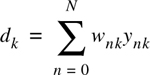
The M decision statistics are weighted to form an overall decision statistic as shown in Figure 7.16. The outputs of the M correlators are denoted as Z₁, Z₂,... and Z_M. They are weighted by α₁, α₂ ... and α_M, respectively. The weighting coefficients are based on the power or the SNR from each correlator output. If the power or SNR is small out of a particular correlator, it will be assigned a small weighting factor. Just as in the case of a maximal ratio combining diversity scheme, the overall signal Z′ is given by

Equation 7.79. 

The weighting coefficients, α_m, are normalized to the output signal power of the correlator in such a way that the coefficients sum to unity, as shown in Equation (7.80)

Equation 7.80. 

As in the case of adaptive equalizers and diversity combining, there are many ways to generate the weighting coefficients. However, due to multiple access interference, RAKE fingers with strong multipath amplitudes will not necessarily provide strong output after correlation. Choosing weighting coefficients based on the actual outputs of the correlators yields better RAKE performance.

Interleaving is used to obtain time diversity in a digital communications system without adding any overhead. Interleaving has become an extremely useful technique in all second and third generation wireless systems, due to the rapid proliferation of digital speech coders which transform analog voices into efficient digital messages that are transmitted over wireless links (speech coders are presented in Chapter 8).

Because speech coders attempt to represent a wide range of voices in a uniform and efficient digital format, the encoded data bits (called source bits) carry a great deal of information, and as explained in Chapters 8 and 11, some source bits are more important than others and must be protected from errors. It is typical for many speech coders to produce several “important” bits in succession, and it is the function of the interleaver to spread these bits out in time so that if there is a deep fade or noise burst, the important bits from a block of source data are not corrupted at the same time. By spreading the source bits over time, it becomes possible to make use of error control coding (called channel coding) which protects the source data from corruption by the channel. Since error control codes are designed to protect against channel errors that may occur randomly or in a bursty manner, interleavers scramble the time order of source bits before they are channel coded.

An interleaver can be one of two forms—a block structure or a convolutional structure. A block interleaver formats the encoded data into a rectangular array of m rows and n columns, and interleaves nm bits at a time. Usually, each row contains a word of source data having n bits. An interleaver of degree m (or depth m) consists of m rows. The structure of a block interleaver is shown in Figure 7.17. As seen, source bits are placed into the interleaver by sequentially increasing the row number for each successive bit, and filling the columns. The interleaved source data is then read out row-wise and transmitted over the channel. This has the effect of separating the original source bits by m bit periods.

Figure 7.17. Block interleaver where source bits are read into columns and read out as n-bit rows.

At the receiver, the de-interleaver stores the received data by sequentially increasing the row number of each successive bit, and then clocks out the data row-wise, one word (row) at a time.

Convolutional interleavers can be used in place of block interleavers in much the same fashion. Convolutional interleavers are ideally suited for use with convolutional codes.

There is an inherent delay associated with an interleaver since the received message block cannot be fully decoded until all of the nm bits arrive at the receiver and are de-interleaved. In practice, human speech is tolerable to listen to until delays of greater than 40 ms occur. It is for this reason that all of the wireless data interleavers have delays which do not exceed 40 ms. The interleaver word size and depth are closely related to the type of speech coder used, the source coding rate, and the maximum tolerable delay.

Channel coding protects digital data from errors by selectively introducing redundancies in the transmitted data. Channel codes that are used to detect errors are called error detection codes, while codes that can detect and correct errors are called error correction codes.

In 1948, Shannon demonstrated that by proper encoding of the information, errors induced by a noisy channel can be reduced to any desired level without sacrificing the rate of information transfer [Sha48]. Shannon’s channel capacity formula is applicable to the AWGN channel and is given by

Equation 7.81. 

where C is the channel capacity (bits per second), B is the transmission bandwidth (Hz), P is the received signal power (W), and N₀ is the single-sided noise power density (W/Hz). The received power at a receiver is given as

Equation 7.82. 

where E_b is the average bit energy, and R_b is the transmission bit rate. Equation (7.81) can be normalized by the transmission bandwidth and is given by

Equation 7.83. 

where C/B denotes bandwidth efficiency.

The basic purpose of error detection and error correction techniques is to introduce redundancies in the data to improve wireless link performance. The introduction of redundant bits increases the raw data rate used in the link, and, hence, it increases the bandwidth requirement for a fixed source data rate. This reduces the bandwidth efficiency of the link in high SNR conditions, but provides excellent BER performance at low SNR values.

It is well known that the use of orthogonal signaling allows the probability of error to become arbitrarily small by expanding the signal set, i.e., by making the number of waveforms M → ∞, provided that the SNR per bit exceeds the Shannon limit of SNR_b ≥ −1.6 dB [Vit79]. In the limit, Shannon’s result indicates that extremely wideband signals could be used to achieve error free communications, as long as sufficient SNR exists, and this is partly why wideband CDMA is being adopted for 3G. Error control coding waveforms, on the other hand, have bandwidth expansion factors that grow only linearly with the code block length. Error correction coding thus offers advantages in bandwidth limited applications, and also provides link protection in power limited applications.

A channel coder operates on digital message (source) data by encoding the source information into a code sequence for transmission through the channel. There are three basic types of error correction and detection codes: block codes, convolutional codes, and turbo codes.

Block codes are forward error correction (FEC) codes that enable a limited number of errors to be detected and corrected without retransmission. Block codes can be used to improve the performance of a communications system when other means of improvement (such as increasing transmitter power or using a more sophisticated demodulator) are impractical.

In block codes, parity bits are added to blocks of message bits to make codewords or code blocks. In a block encoder, k information bits are encoded into n code bits. A total of n − k redundant bits are added to the k information bits for the purpose of detecting and correcting errors [Lin83]. The block code is referred to as an (n, k) code, and the rate of the code is defined as R_c = k/n and is equal to the rate of information divided by the raw channel rate.

The ability of a block code to correct errors is a function of the code distance. Many families of codes exist that provide varying degrees of error protection [Cou93], [Hay94], [Lin83], [Skl93], and [Vit79].

Besides the code rate, other important parameters are the code distance and the weight of particular codewords. These are defined below.

Distance of a Code—. The distance between two codewords is the number of elements in which two codewords C_i and C_j differ

Equation 7.84. 

where d is the distance between the codewords and q is the total number of possible values of C_i and C_j. The length of each codeword is N elements or characters. If the code used is binary, the distance is known as the Hamming distance. The minimum distance d_min is the smallest distance for the given codeword set and is given as

Equation 7.85. 

Weight of a Code—. The weight of a codeword of length N is given by the number of nonzero elements in the codeword. For a binary code, the weight is basically the number of 1s in the codeword and is given as

Equation 7.86. 

Properties of Block Codes

Linearity—. Suppose C_i and C_j are two codewords in an (n,k) block code. Let α₁ and α₂ be any two elements selected from the alphabet. Then the code is said to be linear if and only if α₁C₁ + α₂C₂ is also a code word. A linear code must contain the all-zero code word. Consequently, a constant-weight code is nonlinear.

Systematic—. A systematic code is one in which the parity bits are appended to the end of the information bits. For an (n,k) code, the first k bits are identical to the information bits, and the remaining n – k bits of each code word are linear combinations of the k information bits.

Cyclic—. Cyclic codes are a subset of the class of linear codes, which satisfy the following cyclic shift property: If C = [c_{n − 1,} c_{n − 2,} ....., c₀] is a codeword of a cyclic code, then [c_{n − 2}, c_{n − 3}, ....., c₀, c_{n − 1}], obtained by a cyclic shift of the elements of C, is also a code word. That is, all cyclic shifts of C are code words. As a consequence of the cyclic property, the codes possess a considerable amount of structure which can be exploited to greatly simplify the encoding and decoding operations.

Encoding and decoding techniques make use of the mathematical constructs know as finite fields. Finite fields are algebraic systems which contain a finite set of elements. Addition, subtraction, multiplication, and division of finite field elements is accomplished without leaving the set (i.e., the sum/product of two field elements is a field element). Addition and multiplication must satisfy the commutative, associative, and distributive laws. A formal definition of a finite field is given below:

Let F be a finite set of elements on which two binary operations—addition and multiplication—are defined. The set F together with the two binary operations is a field if the following conditions are satisfied:

• F is a commutative group under addition. The identity element with respect to addition is called the zero element and is denoted by 0.

• The set of nonzero elements in F is a commutative group under multiplication. The identity element with respect to multiplication is called the unit element and is denoted by 1.

• Multiplication is distributive over addition; that is, for any three elements a, b, and c in F:

  a · (b + c) = a · b + a · c

The additive inverse of a field element a, denoted by -a, is the field element which produces the sum 0 when added to a [so that a + (−a) = 0 ]. The multiplicative inverse of a, denoted by a^-1, is the field element which produces the product 1 when multiplied by a [so that a · a^-1 = 1].

Four basic properties of fields can be derived from the definition of a field. They are as follows:

Property I:	a · 0 = 0 = 0 · a
Property II:	For nonzero field elements a and b, a · b ≠ 0
Property III:	a · b = 0 and a ≠ 0 imply b = 0
Property IV:	–(a · b) = (−a) · b = a · (−b)

For any prime number p, there exists a finite field which contains p elements. This prime field is denoted as GF(p) because finite fields are also called Galois fields, in honor of their discoverer [Lin83]. It is also possible to extend the prime field GF(p) to a field of p^m elements which is called an extension field of GF(p) and is denoted by GF(p^m), where m is a positive integer. Codes with symbols from the binary field GF(2) or its extension field GF(2^m) are most commonly used in digital data transmission and storage systems, since information in these systems is always encoded in binary form in practice.

In binary arithmetic, modulo-2 addition and multiplication are used. This arithmetic is actually equivalent to ordinary arithmetic except that two is considered equal to 0 (1 + 1 = 2 = 0). Note that since 1 + 1 = 0, it follows that 1= −1, and hence for the arithmetic used to generate error control codes, addition is equivalent to subtraction.

Reed–Solomon codes make use of nonbinary fields GF(2^m). These fields have more than two elements and are extensions of the binary field GF(2) = {0, 1}. The additional elements in the extension field GF(2^m) cannot be 0 or 1, since all of the elements must be unique, so a new symbol α is used to represent the other elements in the field. Each nonzero element can be represented by a power of α.

The multiplication operation “·” for the extension field must be defined so that the remaining elements of the field can be represented as sequence of powers of α. The multiplication operation can be used to produce the infinite set of elements F shown below

Equation 7.87. 

To obtain the finite set of elements of GF(2^m) from F, a condition must be imposed on F so that it may contain only 2^m elements and is a closed set under multiplication (i.e., multiplication of two field elements is performed without leaving the set). The condition which closes the set of field elements under multiplication is known as the irreducible polynomial, and it typically takes the following form [Rhe89]:

Equation 7.88. 

Using the irreducible polynomial of Equation (7.88), any element which has a power greater than 2^m − 2 can be reduced to an element with a power less than 2^m − 2 as follows:

Equation 7.89. 

The sequence of elements F thus becomes the following sequence F*, whose nonzero terms are closed under multiplication:

Equation 7.90. 

Take the first 2^m terms of F* and you have the elements of the finite field GF(2^m) in their power representation

Equation 7.91. 

It can be shown that each of the 2^m elements of the finite field can be represented as a distinct polynomial of degree m − 1 or less (the element 0 is represented by the zero polynomial, a polynomial with no nonzero terms) [Rhe89]. Each of the nonzero elements of GF(2^m), can be denoted as a polynomial a_i(x), where at least one of the m coefficients is nonzero

Equation 7.92. 

Addition of two elements of the finite field is then defined as the modulo-2 addition of each of the polynomial coefficients of like powers, as shown below

Equation 7.93. 

Thus, GF(2^m) may be constructed, and using Equations (7.92) and (7.93) the polynomial representation for the 2^m elements of the field may be obtained.

Examples of Block Codes

Hamming Codes

Hamming codes were among the first of the nontrivial error correction codes [Ham50]. These codes and their variations have been used for error control in digital communication systems. There are both binary and nonbinary Hamming codes. A binary Hamming code has the property that

Equation 7.94. 

where k is the number of information bits used to form a n bit codeword, and m is any positive integer. The number of parity symbols are n − k = m.

Hadamard Codes

Hadamard codes are obtained by selecting as codewords the rows of a Hadamard matrix. A Hadamard matrix A is a N × N matrix of 1s and 0s, such that each row differs from any other row in exactly N/2 locations. One row contains all zeros with the remainder containing N/2 zeros and N/2 ones. The minimum distance for these codes is N/2.

For N = 2, the Hadamard matrix A is

Equation 7.95. 

In addition to the special case considered above when N = 2^m (m being a positive integer), Hadamard codes of other block lengths are possible, but the codes are not linear.

Golay Codes

Golay codes are linear binary (23,12) codes with a minimum distance of seven and a error correction capability of three bits [Gol49]. This is a special, one of a kind code in that this is the only nontrivial example of a perfect code. (Hamming codes and some repetition codes are also perfect.) Every codeword lies within distance three of any codeword, thus making maximum likelihood decoding possible.

Cyclic Codes

Cyclic codes are a subset of the class of linear codes which satisfy the cyclic property as discussed before. As a result of this property, these codes possess a considerable amount of structure which can be exploited.

A cyclic code can be generated by using a generator polynomial g(p) of degree (n − k). The generator polynomial of an (n,k) cyclic code is a factor of pⁿ + 1 and has the general form

Equation 7.96. 

A message polynomial x(p) can also be defined as

Equation 7.97. 

where (x_k−1, ...., x₀) represents the k information bits. The resultant codeword c(p) can be written as

Equation 7.98. 

where c(p) is a polynomial of degree less than n.

Encoding for a cyclic code is usually performed by a linear feedback shift register based on either the generator or parity polynomial.

BCH Codes

BCH cyclic codes are among the most important block codes, since they exist for a wide range of rates, achieve significant coding gains, and can be implemented even at high speeds [Bos60]. The block length of the codes is n = 2^m − 1 for m ≥3, and the number of errors that they can correct is bounded by t <(2^m − 1)/2. The binary BCH codes can be generalized to create classes of nonbinary codes which use m bits per code symbol. The most important and common class of nonbinary BCH codes is the family of codes known as Reed–Solomon codes. The (63,47) Reed–Solomon code in US Cellular Digital Packet Data (CDPD) uses m = 6 bits per code symbol.

Reed–Solomon Codes

Reed–Solomon (RS) are nonbinary codes which are capable of correcting errors which appear in bursts and are commonly used in concatenated coding systems [Ree60]. The block length of these codes is n = 2^m − 1. These can be extended to 2^m or 2^m + 1. The number of parity symbols that must be used to correct e errors is n − k = 2e. The minimum distance d_min = 2e + 1. RS codes achieve the largest possible d_min of any linear code.

Case Study: Reed–Solomon Codes for CDPD

For the purpose of explanation, the field choice will be GF(64), since this is the same field used in CDPD systems. CDPD uses m = 6, so each of the 64 field elements is represented by a 6 bit symbol. CDPD packets have 282 user bits in a 378 bit block, and eight six-bit symbols (48 bits) may be corrected per block.

A finite field entity p(X) is introduced in order to map the 64 distinct 6-bit symbols to the elements of the field. An irreducible polynomial p(X) of degree m is said to be primitive if the smallest integer n for which p(X) divides Xⁿ + 1 is n = 2^m − 1. This primitive polynomial p(X) is vital for all coding operations as it defines the field and is typically of the form

Equation 7.99. 

In the case of the Reed–Solomon code used for CDPD, Equation (7.99) is indeed the form of p(X). Primitive polynomials have been tabulated for a wide range of field sizes, so p(X) is a known quantity and is part of the definition of any code. CDPD’s primitive polynomial is

Equation 7.100. 

In order to map symbols to field elements, set the primitive polynomial p(α) = 0. This yields the following result, which closes the set of field elements:

Equation 7.101. 

Table 7.2 shows the proper mapping of 6-bit symbols to field elements and this mapping is used to govern all computations. The field elements of Table 7.2 were generated by first starting with the element 1 (α⁰) and then by multiplying by α to obtain the next field element. Any element which contains an α⁵ term will yield an α⁶ term in the next element, but α⁶ is not in GF(64). The primitive polynomial rule is used to convert α⁶ to α + 1. Also note that α⁶² ·α = α = α⁶³ = α⁰ = 1. This simple result is critical when implementing finite field multiplication in software. Multiplication can be accomplished quickly and efficiently by using modulo 2^m – 1 addition of the powers of the elemental operands. For the (63, 47) Reed–Solomon code used in CDPD systems, multiplication of two field elements corresponds to adding the powers of the two operands modulo-63 to arrive at the power of the product.

Table 7.2. Three Representations of the Elements of GF(64) for CDPD

Power Representation	Polynomial Representation						6-Bit Symbol Representation
0 = α63						0	0	0	0	0	0	0
1 = α0						1	0	0	0	0	0	1
α					x1		0	0	0	0	1	0
α2				x2			0	0	0	1	0	0
α3			x3				0	0	1	0	0	0
α4		x4					0	1	0	0	0	0
α5	x5						1	0	0	0	0	0
α6					x1	1	0	0	0	0	1	1
α7				x2	x1		0	0	0	1	1	0
α8			x3	x2			0	0	1	1	0	0
α9		x4	x3				0	1	1	0	0	0
α10	x5	x4					1	1	0	0	0	0
α11	x5				x1	1	1	0	0	0	1	1
α12				x2		1	0	0	0	1		1
α13			x3		x1		0	0	1	0	1	0
α14		x4		x2			0	1	0	1	0	0
α15	x5		x3				1	0	1	0	0	0
α16		x4			x1	1	0	1	0	0	1	1
α17	x5			x2	x1		1	0	0	1	1	0
α18			x3	x2	x1	1	0	0	1	1	1	1
α19		x4	x3	x2	x1		0	1	1	1	1	0
α20	x5	x4	x3	x2			1	1	1	1	0	0
α21	x5	x4	x3		x1	1	1	1	1	0	1	1
α22	x5	x4		x2		1	1	1	0	1	0	1
α23	x5		x3			1	1	0	1	0	0	1
α24		x4				1	0	1	0	0	0	1
α25	x5				x1		1	0	0	0	1	0
α26				x2	x1	1	0	0	0	1	1	1
α27			x3	x2	x1		0	0	1	1	1	0
α28		x4	x3	x2			0	1	1	1	0	0
α29	x5	x4	x3				1	1	1	0	0	0
α30	x5	x4			x1	1	1	1	0	0	1	1
α31	x5			x2		1	1	0	0	1	0	1
α32			x3			1	0	0	1	0	0	1
α33		x4			x1		0	1	0	0	1	0
α34	x5			x2			1	0	0	1	0	0
α35			x3		x1	1	0	0	1	0	1	1
α36		x4		x2	x1		0	1	0	1	1	0
α37	x5		x3	x2			1	0	1	1	0	0
α38		x4	x3		x1	1	0	1	1	0	1	1
α39	x5	x4		x2	x1		1	1	0	1	1	0
α40	x5		x3	x2	x1	1	1	0	1	1	1	1
α41		x4	x3	x2		1	0	1	1	1	0	1
α42	x5	x4	x3		x1		1	1	1	0	1	0
α43	x5	x4		x2	x1	1	1	1	0	1	1	1
α44	x5		x3	x2		1	1	0	1	1	0	1
α45		x4	x3			1	0	1	1	0	0	1
α46	x5	x4			x1		1	1	0	0	1	0
α47	x5			x2	x1	1	1	0	0	1	1	1
α48			x3	x2		1	0	0	1	1	0	1
α49		x4	x3		x1		0	1	1	0	1	0
α50	x5	x4		x2			1	1	0	1	0	0
α51	x5		x3		x1	1	1	0	1	0	1	1
α52		x4		x2		1	0	1	0	1	0	1
α53	x5		x3		x1		1	0	1	0	1	0
α54		x4		x2	x1	1	0	1	0	1	1	1
α55	x5		x3	x2	x1		1	0	1	1	1	0
α56		x4	x3	x2	x1	1	0	1	1	1	1	1
α57	x5	x4	x3	x2	x1		1	1	1	1	1	0
α58	x5	x4	x3	x2	x1	1	1	1	1	1	1	1
α59	x5	x4	x3	x2		1	1	1	1	1	0	1
α60	x5	x4	x3			1	1	1	1	0	0	1
α61	x5	x4				1	1	1	0	0	0	1
α62	x5					1	1	0	0	0	0	1

Addition in GF(2^m) corresponds to modulo-2 adding the coefficients of the polynomial representation of the elements. Since the coefficients are either 1s or 0s (because the field is an extension of the binary field GF(2)), this can simply be implemented with the bit-wise exclusive-OR of the 6-bit symbol representation of the elemental operands. Some examples of finite field addition in GF(64) are shown below:

Equation 7.102.a. 

Equation 7.102.b. 

Reed–Solomon Encoding

In the discussion of a Reed–Solomon encoder, the following polynomials are used frequently:

• d(x) : raw information polynomial

• p(x) : parity polynomial

• c(x) : codeword polynomial

• g(x) : generator polynomial

• q(x) : quotient polynomial

• r(x) : remainder polynomial

Let

Equation 7.103. 

be the information polynomial which is received before decoding and represents the user data, and let

Equation 7.104. 

be the parity polynomial (c_i are all elements of GF(64)). The encoded RS polynomial can thus be expressed as

Equation 7.105. 

A vector of n field elements (c₀, c₁,.....,c_n−1) is a codeword if and only if it is a multiple of the generator polynomial g(x). The generator polynomial for a t -error, correcting, Reed–Solomon code has the form

Equation 7.106. 

A common method for encoding a cyclic code like an RS code is to derive p(x) by dividing d(x) by g(x). This yields an irrelevant quotient polynomial q(x) and an important polynomial r(x) as follows:

Equation 7.107. 

Thus, using Equation (7.105), the codeword polynomial can be expressed as

Equation 7.108. 

If the parity polynomial is defined as being equal to the negatives of the coefficients of r(x), then it follows that

Equation 7.109. 

Thus, by ensuring that the codeword polynomial is a multiple of the generator polynomial, a Reed–Solomon encoder can be constructed by using Equation (7.108) to obtain p(X). The key to encoding and decoding is to find r(x), the remainder polynomial, which maps to the transmitted data. A straightforward method of obtaining the remainder from the division process by using the monic polynomial g(x) is to connect a shift register according to g(x) as shown in Figure 7.18. Each “+” represents an exclusive-OR of two m-bit numbers, each X represents a multiplication of two m-bit numbers under GF(2^m), where each m-bit register contains an m-bit number denoted by b_i.

Figure 7.18. Reed–Solomon encoding circuit.

Initially, all registers are set to 0, and the switch is set to the data position. Code symbols c_n−1 through c_n-k are sequentially shifted into the circuit and simultaneously transmitted to the output line. As soon as code symbol c_n−k enters the circuit, the switch is flipped to the parity position, and the gate to the feedback network is opened so that no further feedback is provided. At that same instant, the registers b₀ through b_2t−1 contain the parity symbols P₀ through P_2t−1, which correspond directly to the coefficients of the parity polynomial. They can be sequentially shifted to the output to complete the Reed–Solomon encoding process.

Reed–Solomon Decoding

Suppose that a codeword

Equation 7.110. 

is transmitted and that channel errors result in the received codeword

Equation 7.111. 

The error pattern e(x)is the difference between c(x) and r(x). Using Equations (7.110) and (7.111),

Equation 7.112. 

Let the 2t partial syndromes S_i, 1 < i ≤ 2t, be defined as S_i = r(αⁱ) . Since α¹, α², ....., α^2t are roots of each transmitted codeword c(x) (because each codeword is a multiple of the generator polynomial g(x)), it follows that c(αⁱ) = 0 and S_i = c(αⁱ)+e(αⁱ) = e(αⁱ). Thus, it is clear that the 2t partial syndromes S_i depend only on the error pattern e(x) and not on the specific received codeword r(x).

Suppose the error pattern contains k errors (k ≤ t) at locations , where 0 ≤ j₁ <j₂ < ..... <j_k < n − 1. Let the error magnitude at each location be denoted as e_ji. Then e(x) has the form

Equation 7.113. 

Define the set of error locator numbers , i = 1, 2, ....., k. Then the set of 2t partial syndromes yields the following system of equations:

Equation 7.114.a. 

Equation 7.114.b. 

Equation 7.114.c. 

Any algorithm which solves this system of equations is a Reed–Solomon decoding algorithm. The error magnitudes e_ji are found directly, and the error locations can be determined from β_i.

Reed–Solomon decoders can be implemented in hardware, software, or a mix of hardware and software. Hardware implementations are typically very fast, but they cannot be used for a wide variety of Reed–Solomon code sizes. For example, there are several single-chip, Reed–Solomon decoders available which decode codes commonly used in satellite communications, digital video applications, and compact disk technology. Hardware decoders can operate at speeds in excess of 50 Mbits per second, but specific hardware solutions operate with specific symbol definitions, such as 8-bit or 9-bit symbols from GF(255), whereas the (63, 47) Reed–Solomon code used in CDPD systems operates with a 6-bit symbol. Since CDPD operates at a slow data rate of 19.2 kbps, a real-time software implementation of a (63, 47) Reed–Solomon decoder can be achieved. A software approach may be more attractive to a modem developer, because it will have a shorter development time, lower development cost, and greater flexibility.

A typical Reed–Solomon decoder uses five distinct algorithms. The first algorithm calculates the 2t partial syndromes S_i. The second step in the RS decoding process is the Berlekamp–Massey algorithm, which calculates the error locator polynomial σ(x). This polynomial is a function of the error locations in the received codeword r(x), but it does not directly indicate which symbols of the received codeword are in error. A Chien search algorithm is then used to calculate these specific error locations from the error locator polynomial. The fourth step in the decoding process is the calculation of the magnitude of the error at each location. Finally, knowing both the error locations in the received codeword and the magnitude of the error at each location, an error correction algorithm may be implemented to correct up to t errors successfully [Rhe89].

Syndrome Calculation

The syndrome of a cyclic code is typically defined as the remainder obtained by dividing the received codeword r(x) by the generator polynomial g(x). However, for Reed–Solomon codes, 2t partial syndromes are computed. Each partial syndrome S_i is defined as the remainder obtained when dividing the received codeword r(x) by x + αⁱ

Equation 7.115. 

The division of two polynomials results in a quotient polynomial q(x) and a remainder polynomial rem(x). The degree of the remainder rem(x) must be less than the degree of the dividing polynomial p(x). Thus, if p(x) has degree 1 (i.e., p(x) = x + αⁱ), rem(x) must have degree 0. In other words, rem(x) is simply a field element and can be denoted as rem. Thus, the determination of the 2t. partial syndromes begins with the calculation

Equation 7.116. 

Rearranging the above equation yields

Equation 7.117. 

Letting x = αⁱ,

Equation 7.118. 

Thus, the calculation of the 2t partial syndromes S_i can be simplified from a full-blown polynomial division (which is computationally intense) to merely evaluating the received polynomial r(x) at x = αⁱ [Rhe89]:

Equation 7.119. 

where

Equation 7.120. 

Thus, r(αⁱ) has the form

Equation 7.121. 

The evaluation of r(αⁱ) can be implemented very efficiently in software by arranging the function so that it has the following form

Equation 7.122. 

Error Locator Polynomial Calculation

The Reed–Solomon decoding process is simply any implementation which solves Equations (7.114.a) through (7.114.c). These 2t equations are symmetric function in β₁, β₂, ....., β_k, known as power-sum symmetric functions. We now define the polynomial

Equation 7.123. 

The roots of σ(x) are , , ....., , which are the inverses of the error location numbers β_i. Thus, σ(x) is called the error locator polynomial because it indirectly contains the exact locations of each of the errors in r(x). Note that σ(x) is an unknown polynomial whose coefficients must also be determined during the Reed–Solomon decoding process.

The coefficients of σ(x) and the error-location numbers β_i are related by the following equations

Equation 7.124.a. 

Equation 7.124.b. 

Equation 7.124.c. 

Equation 7.124.d. 

The unknown quantities σ_i and β_i can be related to the known partial syndromes S_j by the following set of equations known as Newton’s Identities.

Equation 7.125.a. 

Equation 7.125.b. 

Equation 7.125.c. 

Equation 7.125.d. 

The most common method for determining σ(x) is the Berlekamp–Massey algorithm [Lin83].

Convolutional codes are fundamentally different from block codes in that information sequences are not grouped into distinct blocks and encoded [Vit79]. Instead a continuous sequence of information bits is mapped into a continuous sequence of encoder output bits. This mapping is highly structured, enabling a decoding method considerably different from that of block codes to be employed. It can be argued that convolutional coding can achieve a larger coding gain than can be achieved using a block coding with the same complexity.

A convolutional code is generated by passing the information sequence through a finite state shift register. In general, the shift register contains N k-bit stages and m linear algebraic function generators based on the generator polynomials as shown in Figure 7.19. The input data is shifted into and along the shift register, k bits at a time. The number of output bits for each k bit user input data sequence is n bits. The code rate R_c = k/n. The parameter N is called the constraint length and indicates the number of input data bits that the current output is dependent upon. The constraint length determines how powerful and complex the code is. Following is an outline of the various ways of representing convolutional codes.

Figure 7.19. General block diagram of convolutional encoder.

Generator Matrix—. The generator matrix for a convolutional code can define the code and is semi-infinite since the input is semi-infinite in length. Hence, this is not a convenient way of representing a convolutional code.

Generator Polynomials—. For convolutional codes, we specify a set of n vectors, one for each of the n modulo-2 adders used. Each vector of dimension 2k indicates the connection of the encoder to that modulo-2 adder. A 1 in the ith position of the vector indicates that the corresponding shift register stage is connected and a 0 indicates no connection.

Logic Table—. A logic table or lookup table can be built showing the outputs of the convolutional encoder and the state of the encoder for all of the specific input sequences present in the shift register.

State Diagram—. Since the output of the encoder is determined by the input and the current state of the encoder, a state diagram can be used to represent the encoding process. The state diagram is simply a graph of the possible states of the encoder and the possible transitions from one state to another.

Tree Diagram—. The tree diagram shows the structure of the encoder in the form of a tree with the branches representing the various states and the outputs of the coder.

Trellis Diagram—. Close observation of the tree reveals that the structure repeats itself once the number of stages is greater than the constraint length. It is observed that all branches emanating from two nodes having the same state are identical in the sense that they generate identical output sequences. This means that the two nodes having the same label can be merged. By doing this throughout the tree diagram, we can obtain another diagram called a trellis diagram which is a more compact representation.

The advantage of error control codes, whether they be block codes or convolutional codes, is that they provide a coding gain for the communications link. The coding gain describes how much better the user’s decoded message performs as compared to the raw bit error performance of the coded transmission within the channel. Coding gain is what allows a channel error rate of 10^-2 to support decoded user data rates which are 10^-5 or better.

Each error control code has a particular coding gain, which depends on the particular code, the decoder implementation, and the channel BER probability, P_c. It can be shown that a good approximation for the decoded message error probability, P_B is given by

Equation 7.126. 

where t denotes the number of errors that can be corrected in an (n,k) block code. Thus, given a known channel BER, it is possible to determine the user’s decoded message error rate easily. The coding gain measures the amount of additional SNR that would be required to provide the same BER performance for an uncoded message signal in the same channel conditions.

Trellis coded modulation (TCM) is a technique which combines both coding and modulation to achieve significant coding gains without compromising bandwidth efficiency [Ung87]. TCM schemes employ redundant nonbinary modulation in combination with a finite state encoder which decides the selection of modulation signals to generate coded signal sequences. TCM uses signal set expansion to provide redundancy for coding and to design coding and signal mapping functions jointly so as to maximize directly the free distance (minimum Euclidean distance) between the coded signals. In the receiver, the signals are decoded by a soft decision maximum likelihood sequence decoder. Coding gains as large as 6 dB can be obtained without any bandwidth expansion or reduction in the effective information rate.