
4. Product and Portfolio Management
Introduction
Effective marketing comes from customer knowledge and an understanding of how a product fits customers’ needs. In this chapter, we’ll describe metrics used in product strategy and planning. These metrics address the following questions: What volumes can marketers expect from a new product? How will sales of existing products be affected by the launch of a new offering? Is brand equity increasing or decreasing? What do customers really want, and what are they willing to sacrifice to obtain it?
We’ll start with a section on trial and repeat rates, explaining how these metrics are determined and how they’re used to generate sales forecasts for new products. Because forecasts involve growth projections, we’ll then discuss the difference between year-on-year growth and compound annual growth rates (CAGR). Because growth of one product sometimes comes at the expense of an existing product line, it is important to understand cannibalization metrics. These reflect the impact of new products on a portfolio of existing products.
Next, we’ll cover selected metrics associated with brand equity—a central focus of marketing. Indeed, many of the metrics throughout this book can be useful in evaluating brand equity. Certain metrics, however, have been developed specifically to measure the “health” of brands. This chapter will discuss them.
Although branding strategy is a major aspect of a product offering, there are others, and managers must be prepared to make trade-offs among them, informed by a sense of the “worth” of various features. Conjoint analysis helps identify customers’ valuation of specific product attributes. Increasingly, this technique is used to improve products and to help marketers evaluate and segment new or rapidly growing markets. In the final sections of this chapter, we’ll discuss conjoint analysis from multiple perspectives.
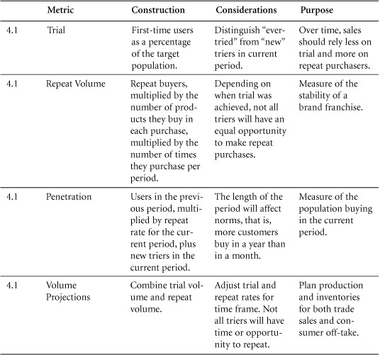
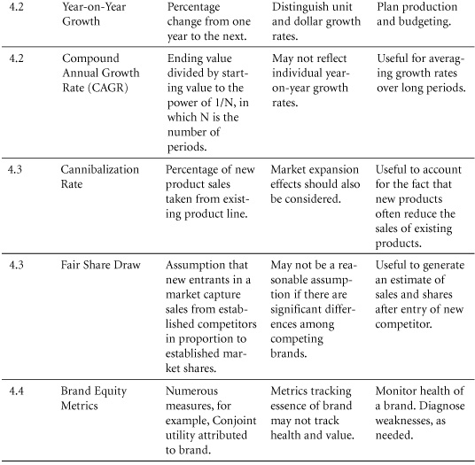
4.1 Trial, Repeat, Penetration, and Volume Projections
Projections from customer surveys are especially useful in the early stages of product development and in setting the timing for product launch. Through such projections, customer response can be estimated without the expense of a full product launch.
Purpose: To understand volume projections.
When projecting sales for relatively new products, marketers typically use a system of trial and repeat calculations to anticipate sales in future periods. This works on the principle that everyone buying the product will either be a new customer (a “trier”) or a repeat customer. By adding new and repeat customers in any period, we can establish the penetration of a product in the marketplace.
It is challenging, however, to project sales to a large population on the basis of simulated test markets, or even full-fledged regional rollouts. Marketers have developed various solutions to increase the speed and reduce the cost of test marketing, such as stocking a store with products (or mock-ups of new products) or giving customers money to buy the products of their choice. These simulate real shopping conditions but require specific models to estimate full-market volume on the basis of test results. To illustrate the conceptual underpinnings of this process, we offer a general model for making volume projection on the basis of test market results.
Construction
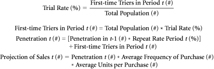
The penetration of a product in a future period can be estimated on the basis of population size, trial rates, and repeat rates.
Trial Rate (%): The percentage of a defined population that purchases or uses a product for the first time in a given period.
First-time Triers in Period t (#): The number of customers who purchase or use a product or brand for the first time in a given period.
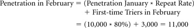
Penetration t (#) = [Penetration in t-1 (#) * Repeat Rate Period t (%)] + First-time Triers in Period t (#)
EXAMPLE: A cable TV company started selling a monthly sports package in January. The company typically has an 80% repeat rate and anticipates that this will continue for the new offering. The company sold 10,000 sports packages in January. In February, it expects to add 3,000 customers for the package. On this basis, we can calculate expected penetration for the sports package in February.
Later that year, in September, the company has 20,000 subscribers. Its repeat rate remains 80%. The company had 18,000 subscribers in August. Management wants to know how many new customers the firm added for its sports package in September:
From penetration, it is a short step to projections of sales.
Projection of Sales (#) = Penetration (#) * Frequency of Purchase (#) * Units per Purchase (#)
Simulated Test Market Results and Volume Projections
Trial Volume
Trial rates are often estimated on the basis of surveys of potential customers. Typically, these surveys ask respondents whether they will “definitely” or “probably” buy a product. As these are the strongest of several possible responses to questions of purchase intentions, they are sometimes referred to as the “top two boxes.” The less favorable responses in a standard five-choice survey include “may or may not buy,” “probably won’t buy,” and “definitely won’t buy.” (Refer to Section 2.7 for more on intention to purchase.)
Because not all respondents follow through on their declared purchase intentions, firms often make adjustments to the percentages in the top two boxes in developing sales projections. For example, some marketers estimate that 80% of respondents who say they’ll “definitely buy” and 30% of those who say that they’ll “probably buy” will in fact purchase a product when given the opportunity.1 (The adjustment for customers following through is used in the following model.) Although some respondents in the bottom three boxes might buy a product, their number is assumed to be insignificant. By reducing the score for the top two boxes, marketers derive a more realistic estimate of the number of potential customers who will try a product, given the right circumstances. Those circumstances are often shaped by product awareness and availability.
Awareness: Sales projection models include an adjustment for lack of awareness of a product within the target market (see Figure 4.1). Lack of awareness reduces the trial rate because it excludes some potential customers who might try the product but don’t know about it. By contrast, if awareness is 100%, then all potential customers know about the product, and no potential sales are lost due to lack of awareness.
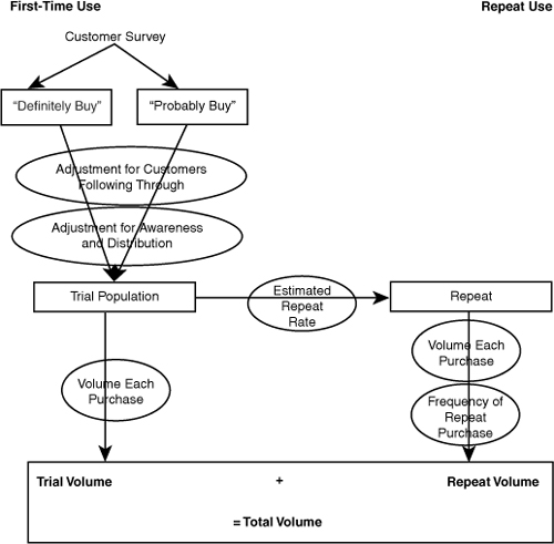
Figure 4.1 Schematic of Simulated Test Market Volume Projection
Distribution: Another adjustment to test market trial rates is usually applied—accounting for the estimated availability of the new product. Even survey respondents who say they’ll “definitely” try a product are unlikely to do so if they can’t find it easily. In making this adjustment, companies typically use an estimated distribution, a percentage of total stores that will stock the new product, such as ACV % distribution. (See Section 6.6 for further detail.)
Adjusted Trial Rate (%) = Trial Rate (%) * Awareness (%) * ACV (%)
After making these modifications, marketers can calculate the number of customers who are expected to try the product, simply by applying the adjusted trial rate to the target population.
Trial Population (#) = Target Population (#) * Adjusted Trial Rate (%)
Estimated in this way, trial population (#) is identical to penetration (#) in the trial period.
To forecast trial volume, multiply trial population by the projected average number of units of a product that will be bought in each trial purchase. This is often assumed to be one unit because most people will experiment with a single unit of a new product before buying larger quantities.
Trial Volume (#) = Trial Population (#) * Units per Purchase (#)
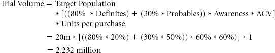
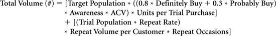
Combining all these calculations, the entire formula for trial volume is
Trial Volume (#) = Target Population (#) * [(80% * Definitely Buy (#)) + (30% * Probably Buy (#)) * Awareness (%) * ACV (%)] * Units per Purchase (#)
EXAMPLE: The marketing team of an office supply manufacturer has a great idea for a new product—a safety stapler. To sell the idea internally, they want to project the volume of sales they can expect over the stapler’s first year. Their customer survey yields the following results (see Table 4.1).
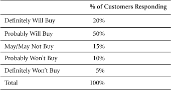
Table 4.1 Customer Survey Responses
On this basis, the company estimates a trial rate for the new stapler by applying the industry-standard expectation that 80% of “definites” and 30% of “probables” will in fact buy the product if given the opportunity.
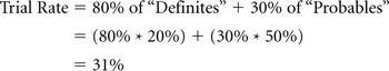
Thus, 31% of the population is expected to try the product if they are aware of it and if it is available in stores. The company has a strong advertising presence and a solid distribution network. Consequently, its marketers believe they can obtain an ACV of approximately 60% for the stapler and that they can generate awareness at a similar level. On this basis, they project an adjusted trial rate of 11.16% of the population:
The target population comprises 20 million people. The trial population can be calculated by multiplying this figure by the adjusted trial rate.
Assuming that each person buys one unit when trying the product, the trial volume will total 2.232 million units.
We can also calculate the trial volume by using the full formula:
Repeat Volume
The second part of projected volume concerns the fraction of people who try a product and then repeat their purchase decision. The model for this dynamic uses a single estimated repeat rate to yield the number of customers who are expected to purchase again after their initial trial. In reality, initial repeat rates are often lower than subsequent repeat rates. For example, it is not uncommon for 50% of trial purchasers to make a first repeat purchase, but for 80% of those who purchase a second time to go on to purchase a third time.

To calculate the repeat volume, the repeat buyers figure can then be multiplied by an expected volume per purchase among repeat customers and by the number of times these customers are expected to repeat their purchases within the period under consideration.
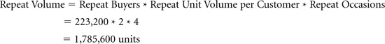
Repeat Volume (#) = Repeat Buyers (#) * Repeat Unit Volume per Customer (#) * Repeat Occasions (#)
This calculation yields the total volume that a new product is expected to generate among repeat customers over a specified introductory period. The full formula can be written as
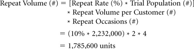
Repeat Volume (#) = [Trial Population (#) * Repeat Rate (%)] * Repeat Unit Volume per Customer (#) * Repeat Occasions (#)
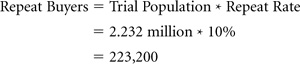
EXAMPLE: Continuing the previous office supplies example, the safety stapler has a trial population of 2.232 million. Marketers expect the product to be of sufficient quality to generate a 10% repeat rate in its first year. This will yield 223,200 repeat buyers:
On average, the company expects each repeat buyer to purchase on four occasions during the first year. On average, each purchase is expected to comprise two units.
This can be represented in the full formula:
Total Volume
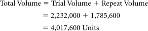
Total volume is the sum of trial volume and repeat volume, as all volume must be sold to either new customers or returning customers.
Total Volume (#) = Trial Volume (#) + Repeat Volume (#)
To capture total volume in its fully detailed form, we need only combine the previous formulas.
EXAMPLE: Total volume in year one for the stapler is the sum of trial volume and repeat volume.
A full calculation of this figure and a template for a spreadsheet calculation are presented in Table 4.2.
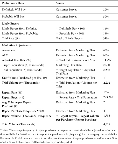
Table 4.2 Volume Projection Spreadsheet
Data Sources, Complications, and Cautions
Sales projections based on test markets will always require the inclusion of key assumptions. In setting these assumptions, marketers face tempting opportunities to make the assumptions fit the desired outcome. Marketers must guard against that temptation and perform sensitivity analysis to establish a range of predictions.
Relatively simple metrics such as trial and repeat rates can be difficult to capture in practice. Although strides have been made in gaining customer data—through customer loyalty cards, for example—it will often be difficult to determine whether customers are new or repeat buyers.
Regarding awareness and distribution: Assumptions concerning the level of public awareness to be generated by launch advertising are fraught with uncertainty. Marketers are advised to ask: What sort of awareness does the product need? What complementary promotions can aid the launch?
Trial and repeat rates are both important. Some products generate strong results in the trial stage but fail to maintain ongoing sales. Consider the following example.
EXAMPLE: Let’s compare the safety stapler with a new product, such as an enhanced envelope sealer. The envelope sealer generates less marketing buzz than the stapler but enjoys a greater repeat rate. To predict results for the envelope sealer, we have adapted the data from the safety stapler by reducing the top two box responses by half (reflecting its lower initial enthusiasm) and raising the repeat rate from 10% to 33% (showing stronger product response after use).
At the six-month mark, sales results for the safety stapler (Product A) are superior to those for the envelope sealer (Product B). After one year, sales results for the two products are equal. On a three-year time scale, however, the envelope sealer—with its loyal base of customers—emerges as the clear winner in sales volume (see Figure 4.2).
The data for the graph is derived as shown in Table 4.3.
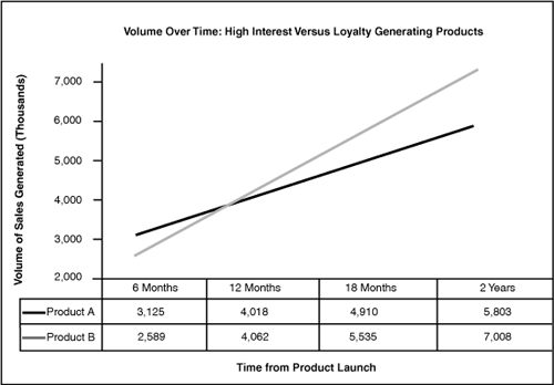
Figure 4.2 Time Horizon Influences Perceived Results
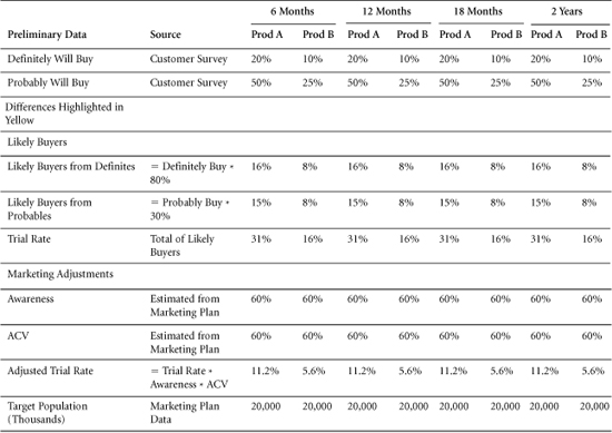
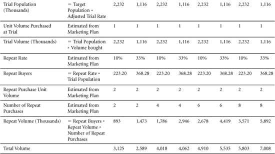
Table 4.3 High Initial Interest or Long-Term Loyalty—Results over Time
Repeating and Trying: Some models assume that customers, after they stop repeating purchases, are lost and do not return. However, customers may be acquired, lost, reacquired, and lost again. In general, the trial-repeat model is best suited to projecting sales over the first few periods. Other means of predicting volume include share of requirements and penetration metrics (refer to Sections 2.4 and 2.5). Those approaches may be preferable for products that lack reliable repeat rates.
Related Metrics and Concepts
Ever-Tried: This is slightly different from trial in that it measures the percentage of the target population that has “ever” (in any previous period) purchased or consumed the product under study. Ever-tried is a cumulative measure and can never add up to more than 100%. Trial, by contrast, is an incremental measure. It indicates the percentage of the population that tries the product for the first time in a given period. Even here, however, there is potential for confusion. If a customer stops buying a product but tries it again six months later, some marketers will categorize that individual as a returning purchaser, others as a new customer. By the latter definition, if individuals can “try” a product more than once, then the sum of all “triers” could equal more than the total population. To avoid confusion, when reviewing a set of data, it’s best to clarify the definitions behind it.
Variations on Trial: Certain scenarios reduce the barriers to trial but entail a lower commitment by the customer than a standard purchase.
• Forced Trial: No other similar product is available. For example, many people who prefer Pepsi-Cola have “tried” Coca-Cola in restaurants that only serve the latter, and vice versa.
• Discounted Trial: Consumers buy a new product but at a substantially reduced price.
Forced and discounted trials are usually associated with lower repeat rates than trials made through volitional purchase.
Evoked Set: The set of brands that consumers name in response to questions about which brands they consider (or might consider) when making a purchase in a specific category. Evoked Sets for breakfast cereals, for example, are often quite large, while those for coffee may be smaller.
Number of New Products: The number of products introduced for the first time in a specific time period.
Revenue from New Products: Usually expressed as the percentage of sales generated by products introduced in the current period or, at times, in the most recent three to five periods.
Margin on New Products: The dollar or percentage profit margin on new products. This can be measured separately but does not differ mathematically from margin calculations.
Company Profit from New Products: The percentage of company profits that is derived from new products. In working with this figure, it is important to understand how “new product” is defined.
Target Market Fit: Of customers purchasing a product, target market fit represents the percentage who belong in the demographic, psychographic, or other descriptor set for that item. Target market fit is useful in evaluating marketing strategies. If a large percentage of customers for a product belongs to groups that have not previously been targeted, marketers may reconsider their targets—and their allocation of marketing spending.
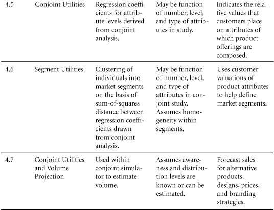
4.2 Growth: Percentage and CAGR
Same stores growth = Growth calculated only on the basis of stores that were fully established in both the prior and current periods.
Purpose: To measure growth.
Growth is the aim of virtually all businesses. Indeed, perceptions of the success or failure of many enterprises are based on assessments of their growth. Measures of year-on-year growth, however, are complicated by two factors:
1. Changes over time in the base from which growth is measured. Such changes might include increases in the number of stores, markets, or salespeople generating sales. This issue is addressed by using “same store” measures (or corollary measures for markets, sales personnel, and so on).
2. Compounding of growth over multiple periods. For example, if a company achieves 30% growth in one year, but its results remain unchanged over the two subsequent years, this would not be the same as 10% growth in each of three years. CAGR, the compound annual growth rate, is a metric that addresses this issue.
Construction
Percentage growth is the central plank of year-on-year analysis. It addresses the question: What has the company achieved this year, compared to last year? Dividing the results for the current period by the results for the prior period will yield a comparative figure. Subtracting one from the other will highlight the increase or decrease between periods. When evaluating comparatives, one might say that results in Year 2 were, for example, 110% of those in Year 1. To convert this figure to a growth rate, one need only subtract 100%.
The periods considered are often years, but any time frame can be chosen.
EXAMPLE: Ed’s is a small deli, which has had great success in its second year of operation. Revenues in Year 2 are $570,000, compared with $380,000 in Year 1. Ed calculates his second-year sales results to be 150% of first-year revenues, indicating a growth rate of 50%.
Same Stores Growth: This metric is at the heart of retail analysis. It enables marketers to analyze results from stores that have been in operation for the entire period under consideration. The logic is to eliminate the stores that have not been open for the full period to ensure comparability. Thus, same stores growth sheds light on the effectiveness with which equivalent resources were used in the period under study versus the prior period. In retail, modest same stores growth and high general growth rates would indicate a rapidly expanding organization, in which growth is driven by investment. When both same stores growth and general growth are strong, a company can be viewed as effectively using its existing base of stores.
EXAMPLE: A small retail chain in Bavaria posts impressive percentage growth figures, moving from €58 million to €107 million in sales (84% growth) from one year to the next. Despite this dynamic growth, however, analysts cast doubt on the firm’s business model, warning that its same stores growth measure suggests that its concept is failing (see Table 4.4).
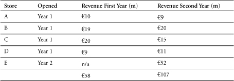
Table 4.4 Revenue of a Bavarian Chain Store
Same stores growth excludes stores that were not open at the beginning of the first year under consideration. For simplicity, we assume that stores in this example were opened on the first day of Years 1 and 2, as appropriate. On this basis, same stores revenue in Year 2 would be €55 million—that is, the €107 million total for the year, less the €52 million generated by the newly opened Store E. This adjusted figure can be entered into the same stores growth formula:
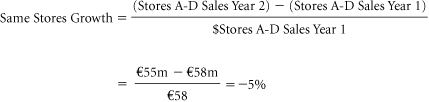
As demonstrated by its negative same stores growth figure, sales growth at this firm has been fueled entirely by a major investment in a new store. This suggests serious doubts about its existing store concept. It also raises a question: Did the new store “cannibalize” existing store sales? (See the next section for cannibalization metrics.)
Compounding Growth, Value at Future Period: By compounding, managers adjust growth figures to account for the iterative effect of improvement. For example, 10% growth in each of two successive years would not be the same as a total of 20% growth over the two-year period. The reason: Growth in the second year is built upon the elevated base achieved in the first. Thus, if sales run $100,000 in Year 0 and rise by 10% in Year 1, then Year 1 sales come to $110,000. If sales rise by a further 10% in Year 2, however, then Year 2 sales do not total $120,000. Rather, they total $110,000 + (10% * $110,000) = $121,000.
The compounding effect can be easily modeled in spreadsheet packages, which enable you to work through the compounding calculations one year at a time. To calculate a value in Year 1, multiply the corresponding Year 0 value by one plus the growth rate. Then use the value in Year 1 as a new base and multiply it by one plus the growth rate to determine the corresponding value for Year 2. Repeat this process through the required number of years.
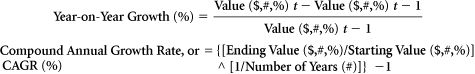
There is a mathematical formula that generates this effect. It multiplies the value at the beginning—that is, in Year 0—by one plus the growth rate to the power of the number of years over which that growth rate applies.
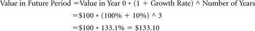
Value in Future Period ($,#,%) = Current Value ($,#,%) * [(1 + CAGR (%)) ^ Number of Periods (#)]
EXAMPLE: Using the formula, we can calculate the impact of 10% annual growth over a period of three years. The value in Year 0 is $100. The number of years is 3. The growth rate is 10%.
Compound Annual Growth Rate (CAGR): The CAGR is a constant year-on-year growth rate applied over a period of time. Given starting and ending values, and the length of the period involved, it can be calculated as follows:
CAGR (%) = {[Ending Value ($,#)/Starting Value ($,#)] ^ 1/Number of Periods (#)} – 1
EXAMPLE: Let’s assume we have the results of the compounding growth observed in the previous example, but we don’t know what the growth rate was. We know that the starting value was $100, the ending value was $133.10, and the number of years was 3. We can simply enter these numbers into the CAGR formula to derive the CAGR.
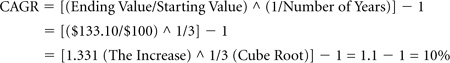
Thus, we determine that the growth rate was 10%.
Data Sources, Complications, and Cautions
Percentage growth is a useful measure as part of a package of metrics. It can be deceiving, however, if not adjusted for the addition of such factors as stores, salespeople, or products, or for expansion into new markets. “Same store” sales, and similar adjustments for other factors, tell us how effectively a company uses comparable resources. These very adjustments, however, are limited by their deliberate omission of factors that weren’t in operation for the full period under study. Adjusted figures must be reviewed in tandem with measures of total growth.
Related Metrics and Concepts
Life Cycle: Marketers view products as passing through four stages of development:
• Introductory: Small markets not yet growing fast.
• Growth: Larger markets with faster growth rates.
• Mature: Largest markets but little or no growth.
• Decline: Variable size markets with negative growth rates.
This is a rough classification. No generally accepted rules exist for making these classifications.
4.3 Cannibalization Rates and Fair Share Draw
Cannibalization rates represent an important factor in the assessment of new product strategies.
Fair share draw constitutes an assumption or expectation that a new product will capture sales (in unit or dollar terms) from existing products in proportion to the market shares of those existing products.
Cannibalization is a familiar business dynamic. A company with a successful product that has strong market share is faced by two conflicting ideas. The first is that it wants to maximize profits on its existing product line, concentrating on the current strengths that promise success in the short term. The second idea is that this company—or its competitors—may identify opportunities for new products that better fit the needs of certain segments. If the company introduces a new product in this field, however, it may “cannibalize” the sales of its existing products. That is, it may weaken the sales of its proven, already successful product line. If the company declines to introduce the new product, however, it will leave itself vulnerable to competitors who will launch such a product, and may thereby capture sales and market share from the company. Often, when new segments are emerging and there are advantages to being early to market, the key factor becomes timing. If a company launches its new product too early, it may lose too much income on its existing line; if it launches too late, it may miss the new opportunity altogether.
Cannibalization: A market phenomenon in which sales of one product are achieved at the expense of some of a firm’s other products.
The cannibalization rate is the percentage of sales of a new product that come from a specific set of existing products.
Any company considering the introduction of a new product should confront the potential for cannibalization. A firm would do well to ensure that the amount of cannibalization is estimated beforehand to provide an idea of how the product line’s contribution as a whole will change. If performed properly, this analysis will tell a company whether overall profits can be expected to increase or decrease with the introduction of the new product line.
EXAMPLE: Lois sells umbrellas on a small beach where she is the only provider. Her financials for last month were as follows:
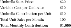
Next month, Lois plans to introduce a bigger, lighter-weight umbrella called the “Big Block.” Projected financials for the Big Block are as follows:
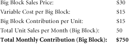
If there is no cannibalization, Lois thus expects her total monthly contribution will be $1,000 + $750, or $1,750. Upon reflection, however, Lois thinks that the unit cannibalization rate for Big Block will be 60%. Her projected financials after accounting for cannibalization are therefore as follows:
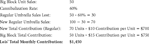
Under these projections, total umbrella sales will increase from 100 to 120, and total contribution will increase from $1,000 to $1,450. Lois will replace 30 regular sales with 30 Big Block sales and gain an extra $5 unit contribution on each. She will also sell 20 more umbrellas than she sold last month and gain $15 unit contribution on each.
In this scenario, Lois was in the enviable position of being able to cannibalize a lower-margin product with a higher-margin one. Sometimes, however, new products carry unit contributions lower than those of existing products. In these instances, cannibalization reduces overall profits for the firm.
An alternative way to account for cannibalization is to use a weighted contribution margin. In the previous example, the weighted contribution margin would be the unit margin Lois receives for Big Block after accounting for cannibalization. Because each Big Block contributes $15 directly and cannibalizes the $10 contribution generated by regular umbrellas at a 60% rate, Big Block’s weighted contribution margin is $15 – (0.6 * $10), or $9 per unit. Because Lois expects to sell 50 Big Blocks, her total contribution is projected to increase by 50 * $9, or $450. This is consistent with our previous calculations.
If the introduction of Big Block requires some fixed marketing expenditure, then the $9 weighted margin can be used to find the break-even number of Big Block sales required to justify that expenditure. For example, if the launch of Big Block requires $360 in one-time marketing costs, then Lois needs to sell $360/$9, or 40 Big Blocks to break even on that expenditure.
If a new product has a margin lower than that of the existing product that it cannibalizes, and if its cannibalization rate is high enough, then its weighted contribution margin might be negative. In that case, company earnings will decrease with each unit of the new product sold.
Cannibalization refers to a dynamic in which one product of a firm takes share from one or more other products of the same firm. When a product takes sales from a competitor’s product, that is not cannibalization … though managers sometimes incorrectly state that their new products are “cannibalizing” sales of a competitor’s goods.
Though it is not cannibalization, the impact of a new product on the sales of competing goods is an important consideration in a product launch. One simple assumption about how the introduction of a new product might affect the sales of existing products is called “fair share draw.”
Fair Share Draw: The assumption that a new product will capture sales (in unit or dollar terms) from existing products in direct proportion to the market shares held by those existing products.
EXAMPLE: Three rivals compete in the youth fashion market in a small town. Their sales and market shares for last year appear in the following table.
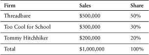
A new entrant is expected to enter the market in the coming year and to generate $300,000 in sales. Two-thirds of those sales are expected to come at the expense of the three established competitors. Under an assumption of fair share draw, how much will each firm sell next year?
If the new firm takes two-thirds of its sales from existing competitors, then this “capture” of sales will total (2/3) * $300,000, or $200,000. Under fair share draw, the breakdown of that $200,000 will be proportional to the shares of the current competitors. Thus 50% of the $200,000 will come from Threadbare, 30% from Too Cool, and 20% from Tommy. The following table shows the projected sales and market shares next year of the four competitors under the fair share draw assumption:
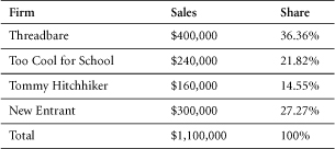
Notice that the new entrant expands the market by $100,000, an amount equal to the sales of the new entrant that do not come at the expense of existing competitors. Notice also that under fair share draw, the relative shares of the existing competitors remain unchanged. For example, Threadbare’s share, relative to the total of the original three competitors, is 36.36/(36.36 + 21.82 + 14.55), or 50%—equal to its share before the entry of the new competitor.
Data Sources, Complications, and Cautions
As noted previously, in cannibalization, one of a firm’s products takes sales from one or more of that firm’s other products. Sales taken from the products of competitors are not “cannibalized” sales, though some managers label them as such.
Cannibalization rates depend on how the features, pricing, promotion, and distribution of the new product compare to those of a firm’s existing products. The greater the similarity of their respective marketing strategies, the higher the cannibalization rate is likely to be.
Although cannibalization is always an issue when a firm launches a new product that competes with its established line, this dynamic is particularly damaging to the firm’s profitability when a low-margin entrant captures sales from the firm’s higher-margin offerings. In such cases, the new product’s weighted contribution margin can be negative. Even when cannibalization rates are significant, however, and even if the net effect on the bottom line is negative, it may be wise for a firm to proceed with a new product if management believes that the original line is losing its competitive strength. The following example is illustrative.
EXAMPLE: A producer of powdered-milk formula has an opportunity to introduce a new, improved formula. The new formula has certain attributes not found in the firm’s existing products. Due to higher costs, however, it will carry a contribution margin of only $8, compared with the $10 margin of the established formula. Analysis suggests that the unit cannibalization rate of the new formula will be 90% in its initial year. If the firm expects to sell 300 units of the new formula in its first year, should it proceed with the introduction?
Analysis shows that the new formula will generate $8 * 300, or $2,400 in direct contribution. Cannibalization, however, will reduce contribution from the established line by $10 * 0.9 * 300, or $2,700. Thus, the company’s overall contribution will decline by $300 with the introduction of the new formula. (Note also that the weighted unit margin for the new product is – $1.) This simple analysis suggests that the new formula should not be introduced.
The following table, however, contains the results of a more detailed four-year analysis. Reflected in this table are management’s beliefs that without the new formula, sales of the regular formula will decline to 700 units in Year 4. In addition, unit sales of the new formula are expected to increase to 600 in Year 4, while cannibalization rates decline to 60%.
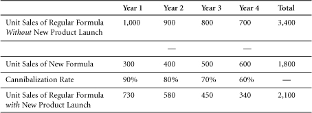
Without the new formula, total four-year contribution is projected as $10 * 3,400, or $34,000. With the new formula, total contribution is projected as ($8 * 1,800) + ($10 * 2,100), or $35,400. Although forecast contribution is lower in Year 1 with the new formula than without it, total four-year contribution is projected to be higher with the new product due to increases in new-formula sales and decreases in the cannibalization rate.
4.4 Brand Equity Metrics
Brand Equity Ten (Aaker)
Brand Asset® Valuator (Young & Rubicam)
Brand Equity Index (Moran)
Brand Valuation Model (Interbrand)
Purpose: To measure the value of a brand.
A brand encompasses the name, logo, image, and perceptions that identify a product, service, or provider in the minds of customers. It takes shape in advertising, packaging, and other marketing communications, and becomes a focus of the relationship with consumers. In time, a brand comes to embody a promise about the goods it identifies— a promise about quality, performance, or other dimensions of value, which can influence consumers’ choices among competing products. When consumers trust a brand and find it relevant, they may select the offerings associated with that brand over those of competitors, even at a premium price. When a brand’s promise extends beyond a particular product, its owner may leverage it to enter new markets. For all these reasons, a brand can hold tremendous value, known as brand equity.
Yet this value can be remarkably difficult to measure. At a corporate level, when one company buys another, marketers might analyze the goodwill component of the purchase price to shed light on the value of the brands acquired. As goodwill represents the excess paid for a firm—beyond the value of its tangible, measurable assets, and as a company’s brands constitute important intangible assets—the goodwill figure may provide a useful indicator of the value of a portfolio of brands. Of course, a company’s brands are rarely the only intangible assets acquired in such a transaction. Goodwill more frequently encompasses intellectual property and other intangibles in addition to brand. The value of intangibles, as estimated by firm valuations (sales or share prices), is also subject to economic cycles, investor “exuberance,” and other influences that are difficult to separate from the intrinsic value of the brand.
From a consumer’s perspective, the value of a brand might be the amount she would be willing to pay for merchandise that carries the brand’s name, over and above the price she’d pay for identical unbranded goods.2 Marketers strive to estimate this premium in order to gain insight into brand equity. Here again, however, they encounter daunting complexities, as individuals vary not only in their awareness of different brands, but in the criteria by which they judge them, the evaluations they make, and the degree to which those opinions guide their purchase behavior.
Theoretically, a marketer might aggregate these preferences across an entire population to estimate the total premium its members would pay for goods of a certain brand. Even that, however, wouldn’t fully capture brand equity. What’s more, the value of a brand encompasses not only the premium a customer will pay for each unit of merchandise associated with that brand, but also the incremental volume it generates. A successful brand will shift outward the demand curve for its goods or services; that is, it not only will enable a provider to charge a higher price (P’ rather than P, as seen in Figure 4.3), but it will also sell an increased quantity (Q’ rather than Q). Thus, brand equity in this example can be viewed as the difference between the revenue with the brand (P’ × Q’) and the revenue without the brand (P × Q)—depicted as the shaded area in Figure 4.3. (Of course, this example focuses on revenue, when, in fact, it is profit or present value of profits that matters more.)
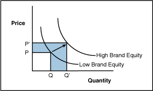
Figure 4.3 Brand Equity—Outward Shift of Demand Curve
In practice, of course, it’s difficult to measure a demand curve, and few marketers do so. Because brands are crucial assets, however, both marketers and academic researchers have devised means to contemplate their value. David Aaker, for example, tracks 10 attributes of a brand to assess its strength. Bill Moran has formulated a brand equity index that can be calculated as the product of effective market share, relative price, and customer retention. Kusum Ailawadi and her colleagues have refined this calculation, suggesting that a truer estimate of a brand’s value might be derived by multiplying the Moran index by the dollar volume of the market in which it competes. Young & Rubicam, a marketing communications agency, has developed a tool called the Brand Asset Valuator©, which measures a brand’s power on the basis of differentiation, relevance, esteem, and knowledge. An even more theoretical conceptualization of brand equity is the difference of the firm value with and without the brand. If you find it difficult to imagine the firm without its brand, then you can appreciate how difficult it is to quantify brand equity. Interbrand, a brand strategy agency, draws upon its own model to separate tangible product value from intangible brand value and uses the latter to rank the top 100 global brands each year. Finally, conjoint analysis can shed light on a brand’s value because it enables marketers to measure the impact of that brand on customer preference, treating it as one among many attributes that consumers trade off in making purchase decisions (see section 4.5).
Construction
Brand Equity Ten (Aaker): David Aaker, a marketing professor and brand consultant, highlights 10 attributes of a brand that can be used to assess its strength. These include Differentiation, Satisfaction or Loyalty, Perceived Quality, Leadership or Popularity, Perceived Value, Brand Personality, Organizational Associations, Brand Awareness, Market Share, and Market Price and Distribution Coverage. Aaker doesn’t weight the attributes or combine them in an overall score, as he believes any weighting would be arbitrary and would vary among brands and categories. Rather, he recommends tracking each attribute separately.
Brand Equity Index (Moran): Marketing executive Bill Moran has derived an index of brand equity as the product of three factors: Effective Market Share, Relative Price, and Durability.
Brand Equity Index (I) = Effective Market Share (%) * Relative Price (I) * Durability (%)
Effective Market Share is a weighted average. It represents the sum of a brand’s market shares in all segments in which it competes, weighted by each segment’s proportion of that brand’s total sales. Thus, if a brand made 70% of its sales in Segment A, in which it had a 50% share of the market, and 30% of its sales in Segment B, in which it had a 20% share, its Effective Market Share would be (0.7 * 0.5) + (0.3 * 0.2) = 0.35 + 0.06 = 0.41, or 41%.
Relative Price is a ratio. It represents the price of goods sold under a given brand, divided by the average price of comparable goods in the market. For example, if goods associated with the brand under study sold for $2.50 per unit, while competing goods sold for an average of $2.00, that brand’s Relative Price would be 1.25, and it would be said to command a price premium. Conversely, if the brand’s goods sold for $1.50, versus $2.00 for the competition, its Relative Price would be 0.75, placing it at a discount to the market. Note that this measure of relative price is not the same as dividing the brand price by the market average price. It does have the advantage that, unlike the latter, the calculated value is not affected by the market share of the firm or its competitors.
Durability is a measure of customer retention or loyalty. It represents the percentage of a brand’s customers who will continue to buy goods under that brand in the following year.
Clearly, marketers can expect to encounter interactions among the three factors behind a Brand Equity Index. If they raise the price of a brand’s goods, for example, they may increase its Relative Price but reduce its Effective Market Share and Durability. Would the overall effect be positive for the brand? By estimating the Brand Equity Index before and after the price increase under consideration, marketers may gain insight into that question.
Notice that two of the factors behind this index, Effective Market Share and Relative Price, draw upon the axes of a demand curve (quantity and price). In constructing his index, Moran has taken those two factors and combined them, through year-to-year retention, with the dimension of time.
Ailawadi, et al suggested that the equity index of a brand can be enhanced by multiplying it by the dollar volume of the market in which the brand competes, generating a better estimate of its value. Ailawadi also contends that the equity of a brand is better captured by its overall revenue premium (relative to generic goods) rather than its price per unit alone, as the revenue figure incorporates both price and quantity and so reflects a jump from one demand curve to another rather than a movement along a single curve.
Brand Asset Valuator (Young & Rubicam): Young & Rubicam, a marketing communications agency, has developed the Brand Asset Valuator, a tool to diagnose the power and value of a brand. In using it, the agency surveys consumers’ perspectives along four dimensions:
• Differentiation: The defining characteristics of the brand and its distinctiveness relative to competitors.
• Relevance: The appropriateness and connection of the brand to a given consumer.
• Esteem: Consumers’ respect for and attraction to the brand.
• Knowledge: Consumers’ awareness of the brand and understanding of what it represents.
Young & Rubicam maintains that these criteria reveal important factors behind brand strength and market dynamics. For example, although powerful brands score high on all four dimensions, growing brands may earn higher grades for Differentiation and Relevance, relative to Knowledge and Esteem. Fading brands often show the reverse pattern, as they’re widely known and respected but may be declining toward commoditization or irrelevance (see Figure 4.4).
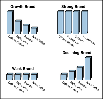
Figure 4.4 Young & Rubicam Brand Asset Valuator Patterns of Brand Equity
The Brand Asset Valuator is a proprietary tool, but the concepts behind it have broad appeal. Many marketers apply these concepts by conducting independent research and exercising judgment about their own brands relative to the competition. Leon Ramsellar3 of Philips Consumer Electronics, for example, has reported using four key measures in evaluating brand equity and offered sample questions for assessing them.
• Uniqueness: Does this product offer something new to me?
• Relevance: Is this product relevant for me?
• Attractiveness: Do I want this product?
• Credibility: Do I believe in the product?
Clearly Ramsellar’s list is not the same as Y&R’s BAV, but the similarity of the first two factors is hard to miss.
Brand Valuation Model (Interbrand): Interbrand, a brand strategy agency, draws upon financial results and projections in its own model for brand valuation. It reviews a company’s financial statements, analyzes its market dynamics and the role of brand in income generation, and separates those earnings attributable to tangible assets (capital, product, packaging, and so on) from the residual that can be ascribed to a brand. It then forecasts future earnings and discounts these on the basis of brand strength and risk. The agency estimates brand value on this basis and tabulates a yearly list of the 100 most valuable global brands.
Conjoint Analysis: Marketers use conjoint analysis to measure consumers’ preference for various attributes of a product, service, or provider, such as features, design, price, or location (see section 4.5). By including brand and price as two of the attributes under consideration, they can gain insight into consumers’ valuation of a brand—that is, their willingness to pay a premium for it.
Data Sources, Complications, and Cautions
The methods described previously represent experts’ best attempts to place a value on a complex and intangible entity. Almost all of the metrics in this book are relevant to brand equity along one dimension or another.
Related Metrics and Concepts
Brand strategy is a broad field and includes several concepts that at first may appear to be measurable. Strictly speaking, however, brand strategy is not a metric.
Brand Identity: This is the marketer’s vision of an ideal brand—the company’s goal for perception of that brand by its target market. All physical, emotional, visual, and verbal messages should be directed toward realization of that goal, including name, logo, signature, and other marketing communications. Brand Identity, however, is not stated in quantifiable terms.
Brand Position and Brand Image: These refer to consumers’ actual perceptions of a brand, often relative to its competition. Brand Position is frequently measured along product dimensions that can be mapped in multi-dimensional space. If measured consistently over time, these dimensions may be viewed as metrics—as coordinates on a perceptual map. (See Section 2.7 for a discussion of attitude, usage measures, and the hierarchy of effects.)
Product Differentiation: This is one of the most frequently used terms in marketing, but it has no universally agreed-upon definition. More than mere “difference,” it generally refers to distinctive attributes of a product that generate increased customer preference or demand. These are often difficult to view quantitatively because they may be actual or perceived, as well as non-monotonic. In other words, although certain attributes such as price can be quantified and follow a linear preference model (that is, either more or less is always better), others can’t be analyzed numerically or may fall into a sweet spot, outside of which neither more nor less would be preferred (the spiciness of a food, for example). For all these reasons, Product Differentiation is hard to analyze as a metric and has been criticized as a “meaningless term.”
Additional Citations
Simon, Julian, “Product Differentiation”: A Meaningless Term and an Impossible Concept, Ethics, Vol. 79, No. 2 (Jan., 1969), pp. 131–138. Published by The University of Chicago Press.
4.5 Conjoint Utilities and Consumer Preference
Conjoint utilities can also play a role in analyzing compensatory and noncompensatory decisions. Weaknesses in compensatory factors can be made up in other attributes. A weakness in a non-compensatory factor cannot be overcome by other strengths.
Conjoint analysis can be useful in determining what customers really want and— when price is included as an attribute—what they’ll pay for it. In launching new products, marketers find such analyses useful for achieving a deeper understanding of the values that customers place on various product attributes. Throughout product management, conjoint utilities can help marketers focus their efforts on the attributes of greatest importance to customers.
Purpose: To understand what customers want.
Conjoint analysis is a method used to estimate customers’ preferences, based on how customers weight the attributes on which a choice is made. The premise of conjoint analysis is that a customer’s preference between product options can be broken into a set of attributes that are weighted to form an overall evaluation. Rather than asking people directly what they want and why, in conjoint analysis, marketers ask people about their overall preferences for a set of choices described on their attributes and then decompose those into the component dimensions and weights underlying them. A model can be developed to compare sets of attributes to determine which represents the most appealing bundle of attributes for customers.
Conjoint analysis is a technique commonly used to assess the attributes of a product or service that are important to targeted customers and to assist in the following:
• Product design
• Advertising copy
• Pricing
• Segmentation
• Forecasting
Construction
Conjoint Analysis: A method of estimating customers by assessing the overall preferences customers assign to alternative choices.
An individual’s preference can be expressed as the total of his or her baseline preferences for any choice, plus the partworths (relative values) for that choice expressed by the individual.
In linear form, this can be represented by the following formula:
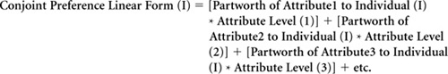
EXAMPLE: Two attributes of a cell phone, its price and its size, are ranked through conjoint analysis, yielding the results shown in Table 4.5.
This could be read as follows:
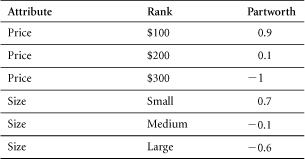
Table 4.5 Conjoint Analysis: Price and Size of a Cell Phone
A small phone for $100 has a partworth to customers of 1.6 (derived as 0.9 + 0.7). This is the highest result observed in this exercise. A small but expensive ($300) phone is rated as –0.3 (that is, –1 + 0.7). The desirability of this small phone is offset by its price. A large, expensive phone is least desirable to customers, generating a partworth of —1.6 (that is, (–1) + ( – 0.6)).
On this basis, we determine that the customer whose views are analyzed here would prefer a medium-size phone at $200 (utility = 0) to a small phone at $300 (utility = –0.3). Such information would be instrumental to decisions concerning the trade-offs between product design and price.
This analysis also demonstrates that, within the ranges examined, price is more important than size from the perspective of this consumer. Price generates a range of effects from 0.9 to – 1 (that is, a total spread of 1.9), while the effects generated by the most and least desirable sizes span a range only from 0.7 to –0.6 (total spread = 1.3).
Compensatory Versus Non-Compensatory Consumer Decisions
A compensatory decision process is one in which a customer evaluates choices with the perspective that strengths along one or more dimensions can compensate for weaknesses along others.
In a non-compensatory decision process, by contrast, if certain attributes of a product are weak, no compensation is possible, even if the product possesses strengths along other dimensions. In the previous cell phone example, for instance, some customers may feel that if a phone were greater than a certain size, no price would make it attractive.
In another example, most people choose a grocery store on the basis of proximity. Any store within a certain radius of home or work may be considered. Beyond that distance, however, all stores will be excluded from consideration, and there is nothing a store can do to overcome this. Even if it posts extraordinarily low prices, offers a stunningly wide assortment, creates great displays, and stocks the freshest foods, for example, a store will not entice consumers to travel 400 miles to buy their groceries.
Although this example is extreme to the point of absurdity, it illustrates an important point: When consumers make a choice on a non-compensatory basis, marketers need to define the dimensions along which certain attributes must be delivered, simply to qualify for consideration of their overall offering.
One form of non-compensatory decision-making is elimination-by-aspect. In this approach, consumers look at an entire set of choices and then eliminate those that do not meet their expectations in the order of the importance of the attributes. In the selection of a grocery store, for example, this process might run as follows:
• Which stores are within 5 miles of my home?
• Which ones are open after 8 p.m.?
• Which carry the spicy mustard that I like?
• Which carry fresh flowers?
The process continues until only one choice is left.
In the ideal situation, in analyzing customers’ decision processes, marketers would have access to information on an individual level, revealing
• Whether the decision for each customer is compensatory or not
• The priority order of the attributes
• The “cut-off” levels for each attribute
• The relative importance weight of each attribute if the decision follows a compensatory process
More frequently, however, marketers have access only to past behavior, helping them make inferences regarding these items.
In the absence of detailed, individual information for customers throughout a market, conjoint analysis provides a means to gain insight into the decision-making processes of a sampling of customers. In conjoint analysis, we generally assume a compensatory process. That is, we assume utilities are additive. Under this assumption, if a choice is weak along one dimension (for example, if a store does not carry spicy mustard), it can compensate for this with strength along another (for example, it does carry fresh-cut flowers) at least in part. Conjoint analyses can approximate a non-compensatory model by assigning non-linear weighting to an attribute across certain levels of its value. For example, the weightings for distance to a grocery store might run as follows:
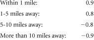
In this example, stores outside a 5-mile radius cannot practically make up the loss of utility they incur as a result of distance. Distance becomes, in effect, a non-compensatory dimension.
By studying customers’ decision-making processes, marketers gain insight into the attributes needed to meet consumer expectations. They learn, for example, whether certain attributes are compensatory or non-compensatory. A strong understanding of customers’ valuation of different attributes also enables marketers to tailor products and allocate resources effectively.
Several potential complications arise in considering compensatory versus noncompensatory decisions. Customers often don’t know whether an attribute is compensatory or not, and they may not be readily able to explain their decisions. Therefore, it is often necessary either to infer a customer’s decision-making process or to determine that process through an evaluation of choices, rather than a description of the process.
It is possible, however, to uncover non-compensatory elements through conjoint analysis. Any attribute for which the valuation spread is so high that it cannot practically be made up by other features is, in effect, a non-compensatory attribute.
Data Sources, Complications, and Cautions
Prior to conducting a conjoint study, it is necessary to identify the attributes of importance to a customer. Focus groups are commonly used for this purpose. After attributes and levels are determined, a typical approach to Conjoint Analysis is to use a fractional factorial orthogonal design, which is a partial sample of all possible combinations of attributes. This is to reduce the total number of choice evaluations required by the respondent. With an orthogonal design, the attributes remain independent of one another, and the test doesn’t weigh one attribute disproportionately to another.
There are multiple ways to gather data, but a straightforward approach would be to present respondents with choices and to ask them to rate those choices according to their preferences. These preferences then become the dependent variable in a regression, in which attribute levels serve as the independent variables, as in the previous equation. Conjoint utilities constitute the weights determined to best capture the preference ratings provided by the respondent.
Often, certain attributes work in tandem to influence customer choice. For example, a fast and sleek sports car may provide greater value to a customer than would be suggested by the sum of the fast and sleek attributes. Such relationships between attributes are not captured by a simple conjoint model, unless one accounts for interactions.
Ideally, conjoint analysis is performed on an individual level because attributes can be weighted differently across individuals. Marketers can also create a more balanced view by performing the analysis across a sample of individuals. It is appropriate to perform the analysis within consumer segments that have similar weights. Conjoint analysis can be viewed as a snapshot in time of a customer’s desires. It will not necessarily translate indefinitely into the future.
It is vital to use the correct attributes in any conjoint study. People can only tell you their preferences within the parameters you set. If the correct attributes are not included in a study, while it may be possible to determine the relative importance of those attributes that are included, and it may technically be possible to form segments on the basis of the resulting data, the analytic results may not be valid for forming useful segments. For example, in a conjoint analysis of consumer preferences regarding colors and styles of cars, one may correctly group customers as to their feelings about these attributes. But if consumers really care most about engine size, then those segmentations will be of little value.
4.6 Segmentation Using Conjoint Utilities
Purpose: To identify segments based on conjoint utilities.
As described in the previous section, conjoint analysis is used to determine customers’ preferences on the basis of the attribute weightings that they reveal in their decisionmaking processes. These weights, or utilities, are generally evaluated on an individual level.
Segmentation entails the grouping of customers who demonstrate similar patterns of preference and weighting with regard to certain product attributes, distinct from the patterns exhibited by other groups. Using segmentation, a company can decide which group(s) to target and can determine an approach to appeal to the segment’s members. After segments have been formed, a company can set strategy based on their attractiveness (size, growth, purchase rate, diversity) and on its own capability to serve these segments, relative to competitors.
Construction
To complete a segmentation based on conjoint utilities, one must first determine utility scores at an individual customer level. Next, one must cluster these customers into segments of like-minded individuals. This is generally done through a methodology known as cluster analysis.
Cluster Analysis: A technique that calculates the distances between customer and forms groups by minimizing the differences within each group and maximizing the differences between groups.
Cluster analysis operates by calculating a “distance” (a sum of squares) between individuals and, in a hierarchical fashion, starts pairing those individuals together. The process of pairing minimizes the “distance” within a group and creates a manageable number of segments within a larger population.
EXAMPLE: The Samson-Finn Company has three customers. In order to help manage its marketing efforts, Samson-Finn wants to organize like-minded customers into segments. Toward that end, it performs a conjoint analysis in which it measures its customers’ preferences among products that are either reliable or very reliable, either fast or very fast (see Table 4.6). It then considers the conjoint utilities of each of its customers to see which of them demonstrate similar wants. When clustering on conjoint data, the distances would be calculated on the partworths.
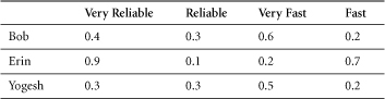
Table 4.6 Customer Conjoint Utilities
The analysis looks at the difference between Bob’s view and Erin’s view on the importance of reliability on their choice. Bob’s score is 0.4 and Erin’s is 0.9. We can square the difference between these to derive the “distance” between Bob and Erin.
Using this methodology, the distance between each pair of Samson-Finn’s customers can be calculated as follows:
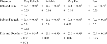
On this basis, Bob and Yogesh appear to be very close to each other because their sum of squares is 0.02. As a result, they should be considered part of the same segment. Conversely, in light of the high sum-of-squares distance established by her preferences, Erin should not be considered a part of the same segment with either Bob or Yogesh.
Of course, most segmentation analyses are performed on large customer bases. This example merely illustrates the process involved in the cluster analysis calculations.
Data Sources, Complications, and Cautions
As noted previously, a customer’s utilities may not be stable, and the segment to which a customer belongs can shift over time or across occasions. An individual might belong to one segment for personal air travel, in which price might be a major factor, and another for business travel, in which convenience might become more important. Such a customer’s conjoint weights (utilities) would differ depending on the purchase occasion.
Determining the appropriate number of segments for an analysis can be somewhat arbitrary. There is no generally accepted statistical means for determining the “correct” number of segments. Ideally, marketers look for a segment structure that fulfills the following qualifications:
• Each segment constitutes a homogeneous group, within which there is relatively little variance between attribute utilities of different individuals.
• Groupings are heterogeneous across segments; that is, there is a wide variance of attribute utilities between segments.
4.7 Conjoint Utilities and Volume Projection
The conjoint utilities of products and services can be used to forecast the market share that each will achieve and the volume that each will sell. Marketers can project market share for a given product or service on the basis of the proportion of individuals who select it from a relevant choice set, as well as its overall utility.
Purpose: To use conjoint analysis to project the market share and the sales volume that will be achieved by a product or service.
Conjoint analysis is used to measure the utilities for a product. The combination of these utilities, generally additive, represents a scoring of sorts for the expected popularity of that product. These scores can be used to rank products. However, further information is needed to estimate market share. One can anticipate that the top-ranked product in a selection set will have a greater probability of being chosen by an individual than products ranked lower for that individual. Adding the number of customers who rank the brand first should allow the calculation of customer share.
Data Sources, Complications, and Cautions
To complete a sales volume projection, it is necessary to have a full conjoint analysis. This analysis must include all the important features according to which consumers make their choice. Defining the “market” is clearly crucial to a meaningful result.
To define a market, it is important to identify all the choices in that market. Calculating the percentage of “first choice” selections for each alternative merely provides a “share of preferences.” To extend this to market share, one must estimate (1) the volume of sales per customer, (2) the level of distribution or availability for each choice, and (3) the percentage of customers who will defer their purchase until they can find their first choice.
The greatest potential error in this process would be to exclude meaningful attributes from the conjoint analysis.
Network effects can also distort a conjoint analysis. In some instances, customers do not make purchase decisions purely on the basis of a product’s attributes but are also affected by its level of acceptance in the marketplace. Such network effects, and the importance of harnessing or overcoming them, are especially evident during shifts in technology industries.
References and Suggested Further Reading
Aaker, D.A. (1991). Managing Brand Equity: Capitalizing on the Value of a Brand Name, New York: Free Press; Toronto; New York: Maxwell Macmillan; Canada: Maxwell Macmillan International.
Aaker, D.A. (1996). Building Strong Brands, New York: Free Press.
Aaker, D.A., and J.M. Carman. (1982). “Are You Overadvertising?” Journal of Advertising Research, 22(4), 57–70.
Aaker, D.A., and K.L. Keller. (1990). “Consumer Evaluations of Brand Extensions,” Journal of Marketing, 54(1), 27–41.
Ailawadi, Kusum, and Kevin Keller. (2004). “Understanding Retail Branding: Conceptual Insights and Research Priorities,” Journal of Retailing, Vol. 80, Issue 4, Winter, 331–342.
Ailawadi, Kusum, Donald Lehman, and Scott Neslin. (2003). “Revenue Premium As an Outcome Measure of Brand Equity,” Journal of Marketing, Vol. 67, No. 4, 1–17.
Burno, Hernan A., Unmish Parthasarathi, and Nisha Singh, eds. (2005). “The Changing Face of Measurement Tools Across the Product Lifecycle,” Does Marketing Measure Up? Performance Metrics: Practices and Impact, Marketing Science Institute, No. 05–301.
Harvard Business School Case: Nestlé Refrigerated Foods Contadina Pasta & Pizza (A) 9–595-035. Rev Jan 30 1997.
Moran, Bill. Personal communication with Paul Farris.