
3. Margins and Profits
Introduction
Peter Drucker has written that the purpose of a business is to create a customer. As marketers, we agree. But we also recognize that a business can’t survive unless it makes a margin as well as a customer. At one level, margins are simply the difference between a product’s price and its cost. This calculation becomes more complicated, however, when multiple variations of a product are sold at multiple prices, through multiple channels, incurring different costs along the way. For example, a recent Business Week article noted that less “than two-thirds of GM’s sales are retail. The rest go to rental-car agencies or to company employees and their families—sales that provide lower gross margins.”1 Although it is still the case that a business can’t survive unless it earns a positive margin, it can be a challenge to determine precisely what margin the firm actually does earn.
In the first section of this chapter, we’ll explain the basic computation of unit and percentage margins, and we’ll introduce the practice of calculating margins as a percentage of selling price.
Next, we’ll show how to “chain” this calculation through two or more levels in a distribution channel and how to calculate end-user purchase price on the basis of a marketer’s selling price. We’ll explain how to combine sales through different channels to calculate average margins and how to compare the economics of different distribution channels.
In the third section, we’ll discuss the use of “statistical” and standard units in tracking price changes over time.
We’ll then turn our attention to measuring product costs, with particular emphasis on the distinction between fixed and variable costs. The margin between a product’s unit price and its variable cost per unit represents a key calculation. It tells us how much the sale of each unit of that product will contribute to covering a firm’s fixed costs. “Contribution margin” on sales is one of the most useful marketing concepts. It requires, however, that we separate fixed from variable costs, and that is often a challenge. Frequently, marketers must take “as a given” which of their firm’s operating and production costs are fixed and which are variable. They are likely, however, to be responsible for making these fixed versus variable distinctions for marketing costs. That is the subject of the fifth section of this chapter.
In the sixth section, we’ll discuss the use of fixed- and variable-cost estimates in calculating the break-even levels of sales and contribution. Finally, we’ll extend our calculation of break-even points, showing how to identify sales and profit targets that are mutually consistent.
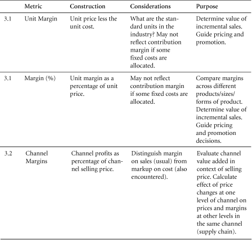
3.1 Margins
Managers need to know margins for almost all marketing decisions. Margins represent a key factor in pricing, return on marketing spending, earnings forecasts, and analyses of customer profitability.
Purpose: To determine the value of incremental sales, and to guide pricing and promotion decisions.
Margin on sales represents a key factor behind many of the most fundamental business considerations, including budgets and forecasts. All managers should, and generally do, know their approximate business margins. Managers differ widely, however, in the assumptions they use in calculating margins and in the ways they analyze and communicate these important figures.
Percentage Margins and Unit Margins: A fundamental variation in the way people talk about margins lies in the difference between percentage margins and unit margins on sales. The difference is easy to reconcile, and managers should be able to switch back and forth between the two.
What is a unit? Every business has its own notion of a “unit,” ranging from a ton of margarine, to 64 ounces of cola, to a bucket of plaster. Many industries work with multiple units and calculate margin accordingly. The cigarette industry, for example, sells “sticks,” “packs,” “cartons,” and 12M “cases” (which hold 1,200 individual cigarettes). Banks calculate margin on the basis of accounts, customers, loans, transactions, households, and branch offices. Marketers must be prepared to shift between such varying perspectives with little effort because decisions can be grounded in any of these perspectives.
Construction
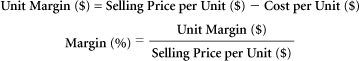
Percentage margins can also be calculated using total sales revenue and total costs.
When working with either percentage or unit margins, marketers can perform a simple check by verifying that the individual parts sum to the total.
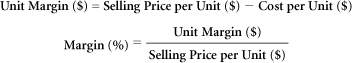
To Verify a Unit Margin ($): Selling Price per Unit = Unit Margin + Cost per Unit
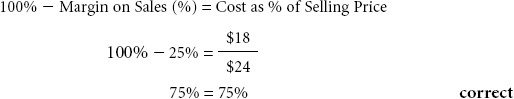
To Verify a Margin (%): Cost as % of Sales = 100%–Margin %
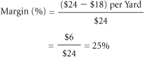
EXAMPLE: A company markets sailcloth by the lineal yard. Its cost basis and selling price for standard cloth are as follows:
Unit Selling Price (Selling Price per Unit) = $24 per Lineal Yard
Unit Cost (Cost per Unit) = $18 per Lineal Yard
To calculate unit margin, we subtract the cost from the selling price:
To calculate the percentage margin, we divide the unit margin by the selling price:
Let’s verify that our calculations are correct:
A similar check can be made on our calculations of percentage margin:
When considering multiple products with different revenues and costs, we can calculate overall margin (%) on either of two bases:
• Total revenue and total costs for all products, or
• The dollar-weighted average of the percentage margins of the different products
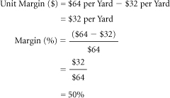
EXAMPLE: The sailcloth company produces a new line of deluxe cloth, which sells for $64 per lineal yard and costs $32 per yard to produce. The margin on this item is 50%.
Because the company now sells two different products, its average margin can only be calculated when we know the volume of each type of goods sold. It would not be accurate to take a simple average of the 25% margin on standard cloth and the 50% margin on deluxe cloth, unless the company sells the same dollar volume of both products.
If, one day, the company sells 20 yards of standard cloth and two yards of deluxe cloth, we can calculate its margins for that day as follows (see also Table 3.1):

Because dollar sales differ between the two products, the company margin of 30% is not a simple average of the margins of those products.
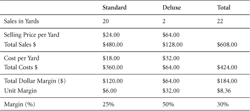
Table 3.1 Sales, Costs, and Margins
Data Sources, Complications, and Cautions
After you determine which units to use, you need two inputs to determine margins: unit costs and unit selling prices.
Selling prices can be defined before or after various “charges” are taken: Rebates, customer discounts, brokers’ fees, and commissions can be reported to management either as costs or as deductions from the selling price. Furthermore, external reporting can vary from management reporting because accounting standards might dictate a treatment that differs from internal practices. Reported margins can vary widely, depending on the calculation technique used. This can result in deep organizational confusion on as fundamental a question as what the price of a product actually is.
Please see Section 8.4 on price waterfalls for cautions on deducting certain discounts and allowances in calculating “net prices.” Often, there is considerable latitude on whether certain items are subtracted from list price to calculate a net price or are added to costs. One example is the retail practice of providing gift certificates to customers who purchase certain amounts of goods. It is not easy to account for these in a way that avoids confusion among prices, marketing costs, and margins. In this context, two points are relevant: (1) Certain items can be treated either as deductions from prices or as increments to cost, but not both. (2) The treatment of such an item will not affect the unit margin, but will affect the percentage margin.
Margin as a percentage of costs: Some industries, particularly retail, calculate margin as a percentage of costs, not of selling prices. Using this technique in the previous example, the percentage margin on a yard of standard sailcloth would be reckoned as the $6.00 unit margin divided by the $18.00 unit cost, or 33%. This can lead to confusion. Marketers must become familiar with the practices in their industry and stand ready to shift between them as needed.
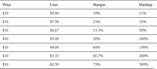
Table 3.2 Relationship Between Margins and Markups
Markup or margin? Although some people use the terms “margin” and “markup” interchangeably, this is not appropriate. The term “markup” commonly refers to the practice of adding a percentage to costs in order to calculate selling prices.
To get a better idea of the relationship between margin and markup, let’s calculate a few. For example, a 50% markup on a variable cost of $10 would be $5, yielding a retail price of $15. By contrast, the margin on an item that sells at a retail price of $15 and that carries a variable cost of $10 would be $5/$15, or 33.3%. Table 3.2 shows some common margin/markup relationships.
One of the peculiarities that can occur in retail is that prices are “marked up” as a percentage of a store’s purchase price (its variable cost for an item) but “marked down” during sales events as a percentage of retail price. Most customers understand that a 50% “sale” means that retail prices have been marked down by 50%.
It is easy to see how confusion can occur. We generally prefer to use the term margin to refer to margin on sales. We recommend, however, that all managers clarify with their colleagues what is meant by this important term.
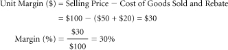
EXAMPLE: A wireless provider sells a handset for $100. The handset costs $50 to manufacture and includes a $20 mail-in rebate. The provider’s internal reports add this rebate to the cost of goods sold. Its margin calculations therefore run as follows:
Accounting standards mandate, however, that external reports deduct rebates from sales revenue (see Table 3.3). Under this construction, the company’s margin calculations run differently and yield a different percentage margin:
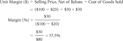
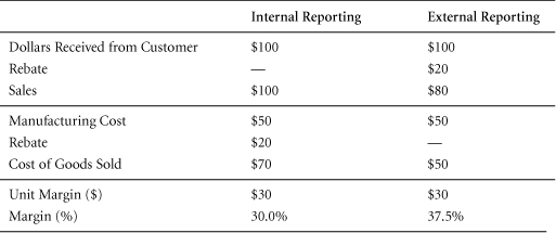
Table 3.3 Internal and External Reporting May Vary
In this example, managers add the rebate to cost of goods sold for the sake of internal reports. In contrast, accounting regulations require that the rebate be deducted from sales for the purpose of external reports. This means that the percentage margin varies between the internal and external reports. This can cause considerable angst within the company when quoting a percentage margin.
As a general principle, we recommend that internal margins follow formats mandated for external reporting in order to limit confusion.
Various costs may or may not be included: The inclusion or exclusion of costs generally depends on the intended purpose of the relevant margin calculations. We’ll return to this issue several times. At one extreme, if all costs are included, then margin and net profit will be equivalent. On the other hand, a marketer may choose to work with “contribution margin” (deducting only variable costs), “operating margin,” or “margin before marketing.” By using certain metrics, marketers can distinguish fixed from variable costs and can isolate particular costs of an operation or of a department from the overall business.
Related Metrics and Concepts
Gross Margin: This is the difference between revenue and cost before accounting for certain other costs. Generally, it is calculated as the selling price of an item, less the cost of goods sold (production or acquisition costs, essentially). Gross margin can be expressed as a percentage or in total dollar terms. If the latter, it can be reported on a per-unit basis or on a per-period basis for a company.
3.2 Prices and Channel Margins
When there are several levels in a distribution chain—including a manufacturer, distributor, and retailer, for example—one must not simply add all channel margins as reported in order to calculate “total” channel margin. Instead, use the selling prices at the beginning and end of the distribution chain (that is, at the levels of the manufacturer and the retailer) to calculate total channel margin. Marketers should be able to work forward from their own selling price to the consumer’s purchase price and should understand channel margins at each step.
Purpose: To calculate selling prices at each level in the distribution channel.
Marketing often involves selling through a series of “value-added” resellers. Sometimes, a product changes form through this progression. At other times, its price is simply “marked up” along its journey through the distribution channel (see Figure 3.1).
In some industries, such as imported beer, there may be as many as four or five channel members that sequentially apply their own margins before a product reaches the consumer. In such cases, it is particularly important to understand channel margins and pricing practices in order to evaluate the effects of price changes.
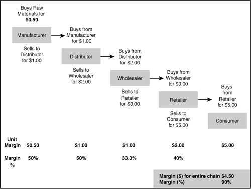
Figure 3.1 Example of a Distribution Channel
Remember: Selling Price = Cost + Margin
Construction
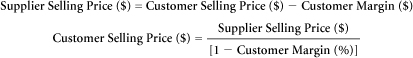
First, decide whether you want to work “backward,” from customer selling prices to supplier selling prices, or “forward.” We provide two equations to use in working backward, one for dollar margins and the other for percentage margins:
Supplier Selling Price ($) = Customer Selling Price ($) – Customer Margin ($)
Supplier Selling Price ($) = Customer Selling Price ($)* [1 – Customer Margin (%)]
EXAMPLE: Aaron owns a small furniture store. He buys BookCo brand bookcases from a local distributor for $200 per unit. Aaron is considering buying directly from BookCo, and he wants to calculate what he would pay if he received the same price that BookCo charges his distributor. Aaron knows that the distributor’s percentage margin is 30%.
The manufacturer supplies the distributor. That is, in this link of the chain, the manufacturer is the supplier, and the distributor is the customer. Thus, because we know the customer’s percentage margin, in order to calculate the manufacturer’s price to Aaron’s distributor, we can use the second of the two previous equations.
Aaron’s distributor buys each bookcase for $140 and sells it for $200, earning a margin of $60 (30%).
Although the previous example may be the most intuitive version of this formula, by rearranging the equation, we can also work forward in the chain, from supplier prices to customer selling prices. In a forward-looking construction, we can solve for the customer selling price, that is, the price charged to the next level of the chain, moving toward the end consumer.2
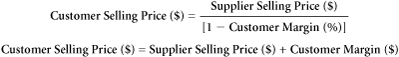
EXAMPLE: Clyde’s Concrete sells 100 cubic yards of concrete for $300 to a road construction contractor. The contractor wants to include this in her bill of materials, to be charged to a local government (see Figure 3.2). Further, she wants to earn a 25% margin. What is the contractor’s selling price for the concrete?

Figure 3.2 Customer Relationships
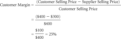
This question focuses on the link between Clyde’s Concrete (supplier) and the contractor (customer). We know the supplier’s selling price is $300 and the customer’s intended margin is 25%. With this information, we can use the first of the two previous equations.
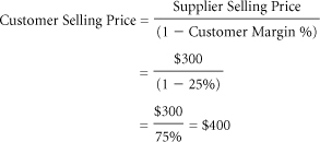
To verify our calculations, we can determine the contractor’s percentage margin, based on a selling price of $400 and a cost of $300.
First Channel Member’s Selling Price: Equipped with these equations and with knowledge of all the margins in a chain of distribution, we can work all the way back to the selling price of the first channel member in the chain.

EXAMPLE: The following margins are received at various steps along the chain of distribution for a jar of pasta sauce that sells for a retail price of $5.00 (see Table 3.4).
What does it cost the manufacturer to produce a jar of pasta sauce? The retail selling price ($5.00), multiplied by 1 less the retailer margin, will yield the wholesaler selling price. The wholesaler selling price can also be viewed as the cost to the retailer. The cost to the wholesaler (distributor selling price) can be found by multiplying the wholesaler selling price by 1 less the wholesaler margin, and so forth. Alternatively, one might follow the next procedure, using a channel member’s percentage margin to calculate its dollar margin, and then subtracting that figure from the channel member’s selling price to obtain its cost (see Table 3.5).
Thus, a jar of pasta that sells for $5.00 at retail actually costs the manufacturer 50 cents to make.
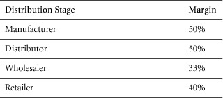
Table 3.4 Example—Pasta Sauce Distribution Margins
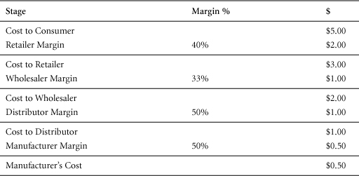
Table 3.5 Cost (Purchase Price) of Retailer
The margins taken at multiple levels of a distribution process can have a dramatic effect on the price paid by consumers. To work backward in analyzing these, many people find it easier to convert markups to margins. Working forward does not require this conversion.
EXAMPLE: To show that margins and markups are two sides of the same coin, let’s demonstrate that we can obtain the same sequence of prices by using the markup method here. Let’s look at how the pasta sauce is marked up to arrive at a final consumer price of $5.00.
As noted previously, the manufacturer’s cost is $0.50. The manufacturer’s percentage markup is 100%. Thus, we can calculate its dollar markup as $0.50 * 100% = $0.50. Adding the manufacturer’s markup to its cost, we arrive at its selling price: $0.50 (cost)+$0.50 (markup) = $1.00. The manufacturer sells the sauce for $1.00 to a distributor. The distributor applies a markup of 100%, taking the price to $2.00, and sells the sauce to a wholesaler. The wholesaler applies a markup of 50% and sells the sauce to a retailer for $3.00. Finally, the retailer applies a markup of 66.7% and sells the pasta sauce to a consumer for $5.00. In Table 3.6, we track these markups to show the pasta sauce’s journey from a manufacturer’s cost of $0.50 to a retail price (consumer’s cost) of $5.00.
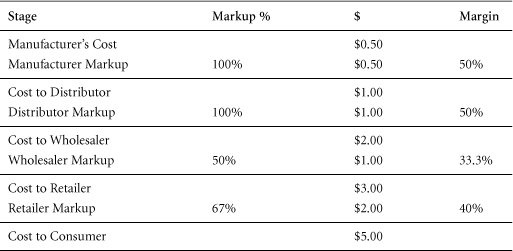
Table 3.6 Markups Along the Distribution Channel
Data Sources, Complications, and Cautions
The information needed to calculate channel margins is the same as for basic margins. Complications arise, however, because of the layers involved. In this structure, the selling price for one layer in the chain becomes the cost to the next layer. This is clearly visible in consumer goods industries, where there are often multiple levels of distribution between the manufacturer and the consumer, and each channel member requires its own margin.
Cost and selling price depend on location within the chain. One must always ask, “Whose cost is this?” and “Who sells at this price?” The process of “chaining” a sequence of margins is not difficult. One need only clarify who sells to whom. In tracking this, it can help first to draw a horizontal line, labeling all the channel members along the chain, with the manufacturer at the far left and the retailer on the right. For example, if a beer exporter in Germany sells to an importer in the U.S., and that importer sells to a distributor in Virginia, who sells the beer to a retailer, then four distinct selling prices and three channel margins will intervene between the exporter and retail store customer. In this scenario, the exporter is the first supplier. The importer is the first customer. To avoid confusion, we recommend mapping out the channel and calculating margins, purchase prices, and selling prices at each level.
Throughout this section, we’ve assumed that all margins are “gross margins,” calculated as selling price minus cost of goods sold. Of course, channel members will incur other costs in the process of “adding value.” If a wholesaler pays his salespeople a commission on sales, for example, that would be a cost of doing business. But it would not be a part of the cost of goods sold, and so it is not factored into gross margin.
Related Metrics and Concepts
Hybrid (Mixed) Channel Margins
Hybrid Channel: The use of multiple distribution systems to reach the same market. A company might approach consumers through stores, the Web, and telemarketing, for example. Margins often differ among such channels. Hybrid channels may also be known as mixed channels.
Increasingly, businesses “go to market” in more than one way. An insurance company, for example, might sell policies through independent agents, toll-free telephone lines, and the Web. Multiple channels often generate different channel margins and cause a supplier to incur different support costs. As business migrates from one channel to another, marketers must adjust pricing and support in economically sensible ways. To make appropriate decisions, they must recognize the more profitable channels in their mix and develop programs and strategies to fit these.
When selling through multiple channels with different margins, it is important to perform analyses on the basis of weighted average channel margins, as opposed to a simple average. Using a simple average can lead to confusion and poor decision-making.
As an example of the variations that can occur, let’s suppose that a company sells 10 units of its product through six channels. It sells five units through one channel ata 20% margin, and one unit through each of the other five channels at a 50% margin. Calculating its average margin on a weighted basis, we arrive at the following figure:
By contrast, if we calculate the average margin among this firm’s six channels on a simple basis, we arrive at a very different figure:
This difference in margin could significantly blur management decision-making.
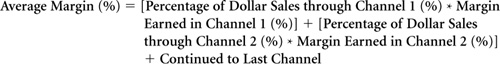
Average Margin
When assessing margins in dollar terms, use percentage of unit sales.

When assessing margin in percentage terms, use percentage of dollar sales.
EXAMPLE: Gael’s Glass sells through three channels: phone, online, and store. These channels generate the following margins: 50%, 40%, and 30%, respectively. When Gael’s wife asks what his average margin is, he initially calculates a simple margin and says it’s 40%. Gael’s wife investigates further, however, and learns that her husband answered too quickly. Gael’s company sells a total of 10 units. It sells one unit by phone at a 50% margin, four units online at a 40% margin, and five units in the store at a 30% margin. To determine the company’s average margin among these channels, the margin in each must be weighted by its relative sales volume. On this basis, Gael’s wife calculates the weighted average margin as follows:

EXAMPLE: Sadetta, Inc. has two channels—online and retail—which generate the following results:
One customer orders online, paying $10 for one unit of goods that costs the company $5. This generates a 50% margin for Sadetta. A second customer shops at the store, buying two units of product for $12 each. Each costs $9. Thus, Sadetta earns a 25% margin on these sales. Summarizing:
Online Margin (1) = 50%. Selling Price (1) = $10. Supplier Selling Price (1) = $5.
Store Margin (2) = 25%. Selling Price (2) = $12. Supplier Selling Price (2) = $9.
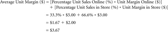
In this scenario, the relative weightings are easy to establish. In unit terms, Sadetta sells a total of three units: one unit (33.3%) online, and two (66.6%) in the store. In dollar terms, Sadetta generates a total of $34 in sales: $10 (29.4%) online, and $24 (70.6%) in the store.
Thus, Sadetta’s average unit margin ($) can be calculated as follows: The online channel generates a $5.00 margin, while the store generates a $3.00 margin. The relative weightings are online 33.3% and store 66.6%.
Sadetta’s average margin (%) can be calculated as follows: The online channel generates a 50% margin, while the store generates a 25% margin. The relative weightings are online 29.4% and store 70.6%.
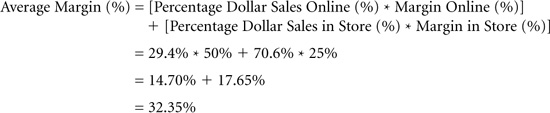
Average margins can also be calculated directly from company totals. Sadetta, Inc. generated a total gross margin of $11 by selling three units of product. Its average unit margin was thus $11/3, or $3.67. Similarly, we can derive Sadetta’s average percentage margin by dividing its total margin by its total revenue. This yields a result that matches our weighted previous calculations: $11/$34 = 32.35%.
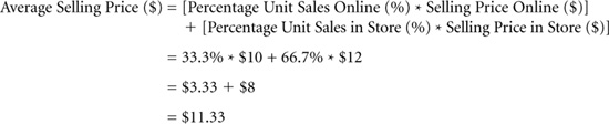
The same weighting process is needed to calculate average selling prices.
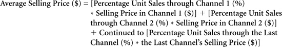
EXAMPLE: Continuing the previous example, we can see how Sadetta, Inc. calculates its average selling price.
Sadetta’s online customer pays $10 per item. Its store customer pays $12 per item. Weighting each channel by unit sales, we can derive Sadetta’s average selling price as follows:
The calculation of average supplier selling price is conceptually similar.
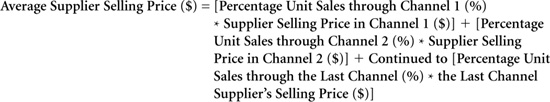
EXAMPLE: Now, let’s consider how Sadetta, Inc. calculates its average supplier selling price.
Sadetta’s online merchandise cost the company $5 per unit. Its in-store merchandise cost $9 per unit. Thus:

With all these pieces of the puzzle, we now have much greater insight into Sadetta, Inc.’s business (see Table 3.7).
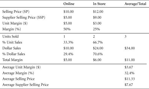
Table 3.7 Sadetta’s Channel Measures
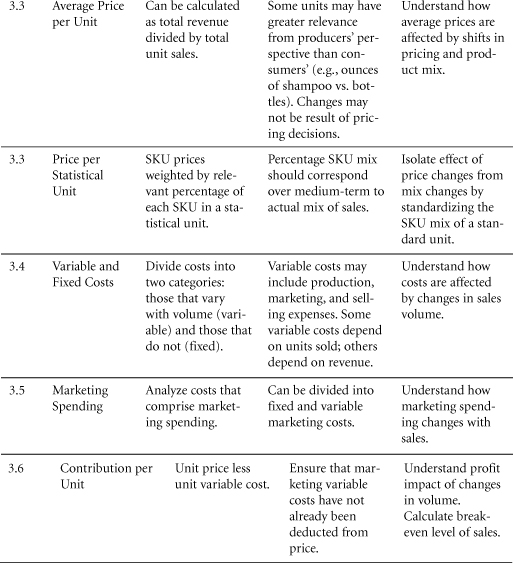
3.3 Average Price per Unit and Price per Statistical Unit
Average prices can be calculated by weighting different unit selling prices by the percentage of unit sales (mix) for each product variant. If we use a standard, rather than an actual mix of sizes and product varieties, the result is price per statistical unit. Statistical units are also known as equivalent units.
Average price per unit and prices per statistical unit are needed by marketers who sellthe same product in different packages, sizes, forms, or configurations at a variety of different prices. As in analyses of different channels, these product and price variations must be reflected accurately in overall average prices. If they are not, marketers may lose sight of what is happening to prices and why. If the price of each product variant remained unchanged, for example, but there was a shift in the mix of volume sold, then the average price per unit would change, but the price per statistical unit would not. Both of these metrics have value in identifying market movements.
Purpose: To calculate meaningful average selling prices within a product line that includes items of different sizes.
Many brands or product lines include multiple models, versions, flavors, colors, sizes, or—more generally—stock keeping units (SKUs). Brita water filters, for example, are sold in a number of SKUs. They are sold in single-filter packs, double-filter packs, and special banded packs that may be restricted to club stores. They are sold on a standalone basis and in combination with pitchers. These various packages and product forms may be known as SKUs, models, items, and so on.
Stock Keeping Unit (SKU): A term used by retailers to identify individual items that are carried or “stocked” within an assortment. This is the most detailed level at which the inventory and sales of individual products are recorded.
Marketers often want to know both their own average prices and those of retailers. By reckoning in terms of SKUs, they can calculate an average price per unit at any level in the distribution chain. Two of the most useful of these averages are
1. A unit price average that includes all sales of all SKUs, expressed as an average price per defined unit. In the water filter industry, for example, these might include such figures as $2.23/filter, $0.03/filtered ounce, and so on.
2. A price per statistical unit that consists of a fixed bundle (number) of individual SKUs. This bundle is often constructed so as to reflect the actual mix of sales of the various SKUs.
The average price per unit will change when there is a shift in the percentage of sales represented by SKUs with different unit prices. It will also change when the prices of the individual SKUs are modified. This contrasts with price per statistical unit, which, by definition, has a fixed proportion of each SKU. Consequently, a price per statistical unit will change only when there is a change in the price of one or more of the SKUs included in it.
The information gleaned from a price per statistical unit can be helpful in considering price movements within a market. Price per statistical unit, in combination with unit price averages, provides insight into the degree to which the average prices in a market are changing as a result of shifts in “mix”—proportions of sales generated by differently priced SKUs—versus price changes for individual items. Alterations in mix—such as a relative increase in the sale of larger versus smaller ice cream tubs at retail grocers, for example—will affect average unit price, but not price per statistical unit. Pricing changes in the SKUs that make up a statistical unit, however, will be reflected by a change in the price of that statistical unit.
Construction
As with other marketing averages, average price per unit can be calculated either from company totals or from the prices and shares of individual SKUs.
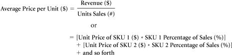
The average price per unit depends on both unit prices and unit sales of individual SKUs. The average price per unit can be driven upward by a rise in unit prices, or by an increase in the unit shares of higher-priced SKUs, or by a combination of the two.
An “average” price metric that is not sensitive to changes in SKU shares is the price per statistical unit.
Price per Statistical Unit
Procter & Gamble and other companies face a challenge in monitoring prices for a wide variety of product sizes, package types, and product formulations. There are as many as 25 to 30 different SKUs for some brands, and each SKU has its own price. In these situations, how do marketers determine a brand’s overall price level in order to compare it to competitive offerings or to track whether prices are rising or falling? One solution is the “statistical unit,” also known as the “statistical case” or—in volumetric or weight measures—the statistical liter or statistical ton. A statistical case of 288 ounces of liquid detergent, for example, might be defined as comprising
Four 4-oz bottles = 16 oz
Twelve 12-oz bottles = 144 oz
Two 32-oz bottles = 64 oz
One 64-oz bottle = 64 oz
Note that the contents of this statistical case were carefully chosen so that it contains the same number of ounces as a standard case of 24 12-ounce bottles. In this way, the statistical case is comparable in size to a standard case. The advantage of a statistical case is that its contents can approximate the mix of SKUs the company actually sells.
Whereas a statistical case of liquid detergent will be filled with whole bottles, in other instances a statistical unit might contain fractions of certain packaging sizes in order for its total contents to match a required volumetric or weight total.
Statistical units are composed of fixed proportions of different SKUs. These fixed proportions ensure that changes in the prices of the statistical unit reflect only changes in the prices of the SKUs that comprise it.
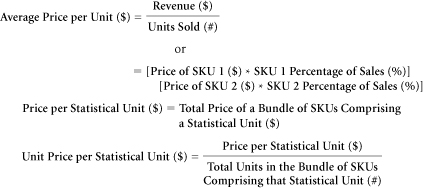
The price of a statistical unit can be expressed either as a total price for the bundle of SKUs comprising it, or in terms of that total price divided by the total volume of its contents. The former might be called the “price per statistical unit”; the latter, the “unit price per statistical unit.”
EXAMPLE: Carl’s Coffee Creamer (CCC) is sold in three sizes: a one-liter economy size, a half-liter “fridge-friendly” package, and a 0.05-liter single serving. Carl defines a 12-liter statistical case of CCC as
Two units of the economy size = 2 liters (2*1.0 liter)
19 units of the fridge-friendly package = 9.5 liters (19*0.5 liter)
Ten single servings = 0.5 liter (10*.05)
Prices for each size and the calculation of total price for the statistical unit are shown in the following table:
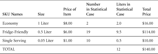
Thus, the total price of the 12-liter statistical case of CCC is $140. The per-liter price within the statistical case is $11.67.
Note that the $140 price of the statistical case is higher than the $96 price of a case of 12 economy packs. This higher price reflects the fact that smaller packages of CCC command a higher price per liter. If the proportions of the SKUs in the statistical case exactly match the actual proportions sold, then the per-liter price of the statistical case will match the per-liter price of the actual liters sold.
EXAMPLE: Carl sells 10,000 one-liter economy packs of CCC, 80,000 fridge-friendly half liters, and 40,000 single servings. What was his average price per liter?
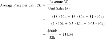
Note that Carl’s average price per liter, at $11.54, is less than the per-liter price in his statistical case. The reason is straightforward: Whereas fridge-friendly packs outnumber economy packs by almost ten to one in the statistical case, the actual sales ratio of these SKUs was only eight to one. Similarly, whereas the ratio of single-serving items to economy items in the statistical case is five to one, their actual sales ratio was only four to one. Carl’s company sold a smaller percentage of the higher (per liter) priced items than was represented in its statistical case. Consequently, its actual average price per liter was less than the per-liter price within its statistical unit.
In the following table, we illustrate the calculation of the average price per unit as the weighted average of the unit prices and unit shares of the three SKUs of Carl’s Coffee Creamer. Unit prices and unit (per-liter) shares are provided.
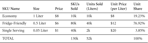
On this basis, the average price per unit ($) = ($8 * 0.1923) + ($12 * 0.7692) + ($20 * 0.0385) = $11.54.
Data Sources, Complications, and Cautions
With complex and changing product lines, and with different selling prices charged by different retailers, marketers need to understand a number of methodologies for calculating average prices. Merely determining how many units of a product are sold, and at what price, throughout the market is a major challenge. As a standard method of tracking prices, marketers use statistical units, which are based on constant proportions of sales of different SKUs in a product line.
Typically, the proportions of SKUs in a statistical unit correspond—at least approximately—to historical market sales. Sales patterns can change, however. In consequence, these proportions need to be monitored carefully in evolving markets and changing product lines.
Calculating a meaningful average price is complicated by the need to differentiate between changes in sales mix and changes in the prices of statistical units. In some industries, it is difficult to construct appropriate units for analyzing price and sales data. In the chemical industry, for example, an herbicide might be sold in a variety of different sizes, applicators, and concentration levels. When we factor in the complexity of different prices and different assortments offered by competing retail outlets, calculating and tracking average prices becomes a non-trivial exercise.
Similar challenges arise in estimating inflation. Economists calculate inflation by using a basket of goods. Their estimates might vary considerably, depending on the goods included. It is also difficult to capture quality improvements in inflation figures. Is a 2009 car, for example, truly comparable to a car built 30 years earlier?
In evaluating price increases, marketers are advised to bear in mind that a consumer who shops for large quantities at discount stores may view such increases very differently from a pensioner who buys small quantities at local stores. Establishing a “standard” basket for such different consumers requires astute judgment. In seeking to summarize the aggregate of such price increases throughout an economy, economists may view inflation as, in effect, a statistical unit price measure for that economy.
3.4 Variable Costs and Fixed Costs
Total Costs ($) = Fixed Costs ($) + Total Variable Costs ($)
Total Variable Costs ($) = Unit Volume (#)*Variable Cost per Unit ($)
Marketers need to have an idea of how costs divide between variable and fixed. This distinction is crucial in forecasting the earnings generated by various changes in unit sales and thus the financial impact of proposed marketing campaigns. It is also fundamental to an understanding of price and volume trade-offs.
Purpose: To understand how costs change with volume.
At first glance, this appears to be an easy subject to master. If a marketing campaign will generate 10,000 units of additional sales, we need only know how much it will cost to supply that additional volume.
The problem, of course, is that no one really knows how changes in quantity will affect a firm’s total costs—in part because the workings of a firm can be so complex. Companies simply can’t afford to employ armies of accountants to answer every possible expense question precisely. Instead, we often use a simple model of cost behavior that is good enough for most purposes.
Construction
The standard linear equation, Y = mX + b, helps explain the relationship between total costs and unit volume. In this application, Y will represent a company’s total cost, m will be its variable cost per unit, X will represent the quantity of products sold (or produced), and b will represent the fixed cost (see Figure 3.3).
Total Cost ($) = Variable Cost per Unit ($)*Quantity (#) + Fixed Cost ($)
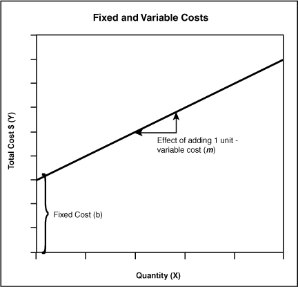
Figure 3.3 Fixed and Variable Costs
On this basis, to determine a company’s total cost for any given quantity of products, we need only multiply its variable cost per unit by that quantity and add its fixed cost.
To communicate fully the implications of fixed costs and variable costs, it may help to separate this graph into two parts (see Figure 3.4).
By definition, fixed costs remain the same, regardless of volume. Consequently, they are represented by a horizontal line across the graph in Figure 3.4. Fixed costs do not increase vertically—that is, they do not add to the total cost—as quantity rises.
The result of multiplying variable cost per unit by quantity is often called the total variable cost. Variable costs differ from fixed costs in that, when there is no production, their total is zero. Their total increases in a steadily rising line, however, as quantity increases.
We can represent this model of cost behavior in a simple equation.
Total Cost ($) = Total Variable Cost ($) + Fixed Cost ($)
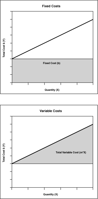
Figure 3.4 Total Cost Consists of Fixed and Variable Costs
To use this model, of course, we must place each of a firm’s costs into one or the other of these two categories. If an expense does not change with volume (rent, for example), then it is part of fixed costs and will remain the same, regardless of how many units the firm produces or sells. If a cost does change with volume (sales commissions, for example), then it is a variable cost.
Total Variable Costs ($) = Unit Volume (#) * Variable Cost per Unit ($)
Total Cost per Unit: It is also possible to express the total cost for a given quantity on a per-unit basis. The result might be called total cost per unit, unit total cost, average cost, full cost, or even fully loaded cost. For our simple linear cost model, the total cost per unit can be calculated in either of two ways. The most obvious would be to divide the total cost by the number of units.
This can be plotted graphically, and it tells an interesting tale (see Figure 3.5). As the quantity rises, the total cost per unit (average cost per unit) declines. The shape of this curve will vary among firms with different cost structures, but wherever there are both fixed and variable costs, the total cost per unit will decline as fixed costs are spread across an increasing quantity of units.
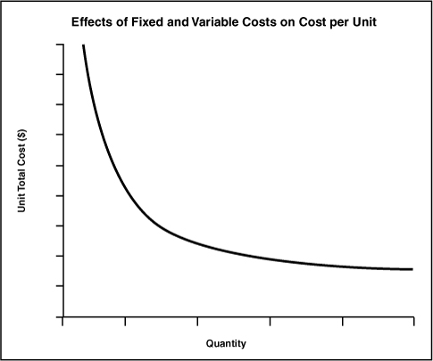
Figure 3.5 Total Cost per Unit Falls with Volume (Typical Assumptions)
The apportionment of fixed costs across units produced leads us to another common formula for the total cost per unit.
Total Cost per Unit ($) = Variable Cost per Unit ($)+[Fixed Cost ($)/Quantity (#)]
As the quantity increases—that is, as fixed costs are spread over an increasing number of units—the total cost per unit declines in a non-linear way.3
EXAMPLE: As a company’s unit sales increase, its fixed costs hold steady at $500. The variable cost per unit remains constant at $10 per unit. Total variable costs increase with each unit sold. The total cost per unit (also known as average total cost) decreases as incremental units are sold and as fixed costs are spread across this rising quantity. Eventually, as more and more units are produced and sold, the company’s total cost per unit approaches its variable cost per unit (see Table 3.8).

Table 3.8 Fixed and Variable Costs at Increasing Volume Levels
In summary, the simplest model of cost behavior is to assume total costs increase linearly with quantity supplied. Total costs are composed of fixed and variable costs. Total cost per unit decreases in a non-linear way with rising quantity supplied.
Data Sources, Complications, and Cautions
Total cost is typically assumed to be a linear function of quantity supplied. That is, the graph of total cost versus quantity will be a straight line. Because some costs are fixed, total cost starts at a level above zero, even when no units are produced. This is because fixed costs include such expenses as factory rent and salaries for full-time employees, which must be paid regardless of whether any goods are produced and sold. Total variable costs, by contrast, rise and fall with quantity. Within our model, however, variable cost per unit is assumed to hold constant—at $10 per unit for example—regardless of whether one unit or 1,000 units are produced. This is a useful model. In using it, however, marketers must recognize that it fails to account for certain complexities.
The linear cost model does not fit every situation: Quantity discounts, expectations of future process improvements, and capacity limitations, for example, introduce dynamics that will limit the usefulness of the fundamental linear cost equation: Total Cost = Fixed Cost + Variable Cost per Unit * Quantity. Even the notion that quantity determines the total cost can be questioned. Although firms pay for inputs, such as raw materials and labor, marketers want to know the cost of the firm’s outputs, that is, finished goods sold. This distinction is clear in theory. In practice, however, it can be difficult to uncover the precise relationship between a quantity of outputs and the total cost of the wide array of inputs that go into it.
The classification of costs as fixed or variable depends on context: Even though the linear model may not work in all situations, it does provide a reasonable approximation for cost behavior in many contexts. Some marketers have trouble, however, with the fact that certain costs can be considered fixed in some contexts and variable in others. In general, for shorter time frames and modest changes in quantity, many costs are fixed. For longer time frames and larger changes in quantity, most costs are variable. Let’s consider rent, for example. Small changes in quantity do not require a change in workspace or business location. In such cases, rent should be regarded as a fixed cost. A major change in quantity, however, would require more or less workspace. Rent, therefore, would become variable over that range of quantity.
Don’t confuse Total Cost per Unit with Variable Cost per Unit: In our linear cost equation, the variable cost per unit is the amount by which total costs increase if the firm increases its quantity by one unit. This number should not be confused with the total cost per unit, calculated as Variable Cost per Unit + (Fixed Cost/Quantity). If a firm has fixed costs, then its total cost per unit will always be greater than the variable cost per unit. Total cost per unit represents the firm’s average cost per unit at the current quantity—and only at the current quantity. Do not make the mistake of thinking of total cost per unit as a figure that applies to changing quantities. Total cost per unit only applies at the volume at which it was calculated.
A related misunderstanding may arise at times from the fact that total cost per unit generally decreases with rising quantity. Some marketers use this fact to argue for aggressively increasing quantity in order to “bring our costs down” and improve profitability. Total cost, by contrast with total cost per unit, almost always increases with quantity. Only with certain quantity discounts or rebates that “kick in” when target volumes are reached can total cost decrease as volume increases.
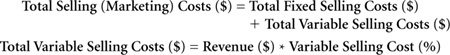
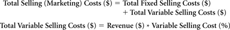
3.5 Marketing Spending—Total, Fixed, and Variable
Recognizing the difference between fixed and variable selling costs can help firms account for the relative risks associated with alternative sales strategies. In general, strategies that incur variable selling costs are less risky because variable selling costs will remain lower in the event that sales fail to meet expectations.
Purpose: To forecast marketing spending and assess budgeting risk.
Marketing Spending: Total expenditure on marketing activities. This typically includes advertising and non-price promotion. It sometimes includes sales force spending and may also include price promotions.
Marketing costs are often a major part of a firm’s overall discretionary expenditures. As such, they are important determinants of short-term profits. Of course, marketing and selling budgets can also be viewed as investments in acquiring and maintaining customers. From either perspective, however, it is useful to distinguish between fixed marketing costs and variable marketing costs. That is, managers must recognize which marketing costs will hold steady, and which will change with sales. Generally, this classification will require a “line-item by line-item” review of the entire marketing budget.
In prior sections, we have viewed total variable costs as expenses that vary with unit sales volume. With respect to selling costs, we’ll need a slightly different conception. Rather than varying with unit sales, total variable selling costs are more likely to vary directly with the monetary value of the units sold—that is, with revenue. Thus, it is more likely that variable selling costs will be expressed as a percentage of revenue, rather than a certain monetary amount per unit.
The classification of selling costs as fixed or variable will depend on an organization’s structure and on the specific decisions of management. A number of items, however, typically fall into one category or the other—with the proviso that their status as fixed or variable can be time-specific. In the long run, all costs eventually become variable.
Over typical planning periods of a quarter or a year, fixed marketing costs might include
• Sales force salaries and support.
• Major advertising campaigns, including production costs.
• Sales promotion material, such as point-of-purchase sales aids, coupon production, and distribution costs.
• Cooperative advertising allowances based on prior-period sales.
Variable marketing costs might include
• Sales commissions paid to sales force, brokers, or manufacturer representatives.
• Sales bonuses contingent on reaching sales goals.
• Off-invoice and performance allowances to trade, which are tied to current volume.
• Early payment terms (if included in sales promotion budgets).
• Coupon face-value payments and rebates, including processing fees.
• Bill-backs for local campaigns, which are conducted by retailers but reimbursed by national brand and cooperative advertising allowances, based on current period sales.
Marketers often don’t consider their budgets in fixed and variable terms, but they can derive at least two benefits by doing so.
First, if marketing spending is in fact variable, then budgeting in this way is more accurate. Some marketers budget a fixed amount and then face an end-of-period discrepancy or “variance” if sales miss their declared targets. By contrast, a flexible budget—that is, one that takes account of its genuinely variable components—will reflect actual results, regardless of where sales end up.
Second, the short-term risks associated with fixed marketing costs are greater than those associated with variable marketing costs. If marketers expect revenues to be sensitive to factors outside their control—such as competitive actions or production shortages—they can reduce risk by including more variable and less fixed spending in their budgets.
A classic decision that hinges on fixed marketing costs versus variable marketing costs is the choice between engaging third-party contract sales representatives versus an in-house sales force. Hiring a salaried—or predominantly salaried—sales force entails more risk than the alternative because salaries must be paid even if the firm fails to achieve its revenue targets. By contrast, when a firm uses third-party brokers to sell its goods on commission, its selling costs decline when sales targets are not met.
Construction
Commissioned Sales Costs: Sales commissions represent one example of selling costs that vary in proportion to revenue. Consequently, any sales commissions should be included in variable selling costs.
There are many types of variable selling costs. For example, selling costs could be based upon a complicated formula, specified in a firm’s contracts with its brokers and dealers. Selling costs might include incentives to local dealers, which are tied to the achievement of specific sales targets. They might include promises to reimburse retailers for spending on cooperative advertising. By contrast, payments to a Web site for a fixed number of impressions or click-throughs, in a contract that calls for specific dollar compensation, would more likely be classified as fixed costs. On the other hand, payments for conversions (sales) would be classified as variable marketing costs.
Data Sources, Complications, and Cautions
Fixed costs are often easier to measure than variable costs. Typically, fixed costs might be assembled from payroll records, lease documents, or financial records. For variable costs, it is necessary to measure the rate at which they increase as a function of activity level. Although variable selling costs often represent a predefined percentage of revenue, they may alternatively vary with the number of units sold (as in a dollar-per-case discount). An additional complication arises if some variable selling costs apply to only a portion of total sales. This can happen, for example, when some dealers qualify for cash discounts or full-truckload rates and some do not.
In a further complication, some expenses may appear to be fixed when they are actually stepped. That is, they are fixed to a point, but they trigger further expenditures beyond that point. For example, a firm may contract with an advertising agency for up to three campaigns per year. If it decides to buy more than three campaigns, it would incur an incremental cost. Typically, stepped costs can be treated as fixed—provided that the boundaries of analysis are well understood.
Stepped payments can be difficult to model. Rebates for customers whose purchases exceed a certain level, or bonuses for salespeople who exceed quota, can be challenging functions to describe. Creativity is important in designing marketing discounts. But this creativity can be difficult to reflect in a framework of fixed and variable costs.
In developing their marketing budgets, firms must decide which costs to expense in the current period and which to amortize over several periods. The latter course is appropriate for expenditures that are correctly viewed as investments. One example of such an investment would be a special allowance for financing receivables from new distributors. Rather than adding such an allowance to the current period’s budget, it would be better viewed as a marketing item that increases the firm’s investment in working capital. By contrast, advertising that is projected to generate long-term impact may be loosely called an investment, but it would be better treated as a marketing expense. Although there may be a valid theoretical case for amortizing advertising, that discussion is beyond the scope of this book.
Related Metrics and Concepts
Levels of marketing spending are often used to compare companies and to demonstrate how heavily they “invest” in this area. For this purpose, marketing spending is generally viewed as a percentage of sales.
Marketing As a Percentage of Sales: The level of marketing spending as a fraction of sales. This figure provides an indication of how heavily a company is marketing. The appropriate level for this figure varies among products, strategies, and markets.
Variants on this metric are used to examine components of marketing in comparison with sales. Examples include trade promotion as a percentage of sales, or sales force as a percentage of sales. One particularly common example is:
Advertising As a Percentage of Sales: Advertising expenditures as a fraction of sales. Generally, this is a subset of marketing as a percentage of sales.
Before using such metrics, marketers are advised to determine whether certain marketing costs have already been subtracted in the calculation of sales revenue. Trade allowances, for example, are often deducted from “gross sales” to calculate “net sales.”
Slotting Allowances: These are a particular form of selling costs encountered when new items are introduced to retailers or distributors. Essentially, they represent a charge made by retailers for making a “slot” available for a new item in their stores and warehouses. This charge may take the form of a one-time cash payment, free goods, or a special discount. The exact terms of the slotting allowance will determine whether it constitutes a fixed or a variable selling cost, or a mix of the two.
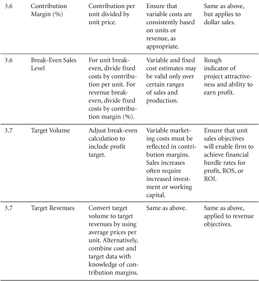
3.6 Break-Even Analysis and Contribution Analysis
Break-even analysis is the Swiss Army knife of marketing economics. It is useful in a variety of situations and is often used to evaluate the likely profitability of marketing actions that affect fixed costs, prices, or variable costs per unit. Break-even is often derived in a “back-of-the-envelope” calculation that determines whether a more detailed analysis is warranted.
Purpose: To provide a rough indicator of the earnings impact of a marketing activity.
The break-even point for any business activity is defined as the level of sales at which neither a profit nor a loss is made on that activity—that is, where Total Revenues = Total Costs. Provided that a company sells its goods at a price per unit that is greater than its variable cost per unit, the sale of each unit will make a “contribution” toward covering some portion of fixed costs. That contribution can be calculated as the difference between price per unit (revenue) and variable cost per unit. On this basis, break-even constitutes the minimum level of sales at which total contribution fully covers fixed costs.
Construction
To determine the break-even point for a business program, one must first calculate the fixed costs of engaging in that program. For this purpose, managers do not need to estimate projected volumes. Fixed costs are constant, regardless of activity level. Managers do, however, need to calculate the difference between revenue per unit and variable costs per unit. This difference represents contribution per unit ($). Contribution rates can also be expressed as a percentage of selling price.
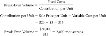
EXAMPLE: Apprentice Mousetraps wants to know how many units of its “Magic Mouse Trapper” it must sell to break even. The product sells for $20. It costs $5 per unit to make. The company’s fixed costs are $30,000. Break-even will be reached when total contribution equals fixed costs.
This dynamic can be summarized in a graph that shows fixed costs, variable costs, total costs, and total revenue (see Figure 3.6). Below the break-even point, total costs exceed total revenue, creating a loss. Above the break-even point, a company generates profits.
Break-Even: Break-even occurs when the total contribution equals the fixed costs. Profits and losses at this point equal zero.
One of the key building blocks of break-even analysis is the concept of contribution. Contribution represents the portion of sales revenue that is not consumed by variable costs and so contributes to the coverage of fixed costs.
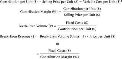
Contribution per Unit ($) = Selling Price per Unit ($) – Variable Cost per Unit ($)
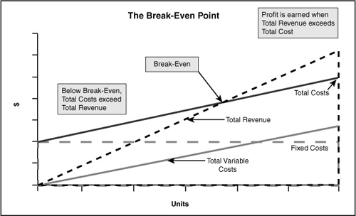
Figure 3.6 At Break-Even, Total Costs = Total Revenues
Contribution can also be expressed in percentage terms, quantifying the fraction of the sales price that contributes toward covering fixed costs. This percentage is often called the contribution margin.
Formulas for total contribution include the following:
As previously noted,
Break-Even Volume: The number of units that must be sold to cover fixed costs.
Break-even will occur when an enterprise sells enough units to cover its fixed costs. If the fixed costs are $10 and the contribution per unit is $2, then a firm must sell five units to break even.
Break-Even Revenue: The level of dollar sales required to break even.
Break-Even Revenue ($) = Break-Even Volume (Units) (#)*Price per Unit ($)
This formula is the simple conversion of volume in units to the revenues generated by that volume.
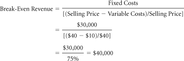
EXAMPLE: Apprentice Mousetraps wants to know how many dollars’ worth of its “Deluxe Mighty Mouse Trapper” it must sell to break even. The product sells for $40 per unit. It costs $10 per unit to make. The company’s fixed costs are $30,000.
With fixed costs of $30,000, and a contribution per unit of $30, Apprentice must sell $30,000/$30 = 1,000 deluxe mousetraps to break even. At $40 per trap, this corresponds to revenues of 1,000*$40 = $40,000.
Break-even in dollar terms can also be calculated by dividing fixed costs by the fraction of the selling price that represents contribution.
Break-even on Incremental Investment
Break-even on incremental investment is a common form of break-even analysis. It examines the additional investment needed to pursue a marketing plan, and it calculates the additional sales required to cover that expenditure. Any costs or revenues that would have occurred regardless of the investment decision are excluded from this analysis.
Data Sources, Complications, and Cautions
To calculate a break-even sales level, one must know the revenues per unit, the variable costs per unit, and the fixed costs. To establish these figures, one must classify all costs as either fixed (those that do not change with volume) or variable (those that increase linearly with volume).
The time scale of the analysis can influence this classification. Indeed, one’s managerial intent can be reflected in the classification. (Will the company fire employees and sublet factory space if sales turn down?) As a general rule, all costs become variable in the long term. Firms generally view rent, for example, as a fixed cost. But in the long term, even rent becomes variable as a company may move into larger quarters when sales grow beyond a certain point.
Before agonizing over these judgments, managers are urged to remember that the most useful application of the break-even exercise is to make a rough judgment about whether more detailed analyses are likely to be worth the effort. The break-even calculation enables managers to judge various options and proposals quickly. It is not, however, a substitute for more detailed analyses, including projections of target profits (Section 3.7), risk, and the time value of money (Sections 5.3 and 10.4).
Related Metrics and Concepts
Payback Period: The period of time required to recoup the funds expended in an investment. The payback period is the time required for an investment to reach break-even (see previous sections).
3.7 Profit-Based Sales Targets
Increasingly, marketers are expected to generate volumes that meet the target profits of their firm. This will often require them to revise sales targets as prices and costs change.
Purpose: To ensure that marketing and sales objectives mesh with profit targets.
In the previous section, we explored the concept of break-even, the point at which a company sells enough to cover its fixed costs. In target volume and target revenue calculations, managers take the next step. They determine the level of unit sales or revenues needed not only to cover a firm’s costs but also to attain its profit targets.
Construction
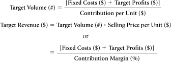
Target Volume: The volume of sales necessary to generate the profits specified in a company’s plans.
The formula for target volume will be familiar to those who have performed break-even analysis. The only change is to add the required profit target to the fixed costs. From another perspective, the break-even volume equation can be viewed as a special case of the general target volume calculation—one in which the profit target is zero, and a company seeks only to cover its fixed costs. In target volume calculations, the company broadens this objective to solve for a desired profit.
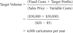
EXAMPLE: Mohan, an artist, wants to know how many caricatures he must sell to realize a yearly profit objective of $30,000. Each caricature sells for $20 and costs $5 in materials to make. The fixed costs for Mohan’s studio are $30,000 per year:
It is quite simple to convert unit target volume to target revenues. One need only multiply the volume figure by an item’s price per unit. Continuing the example of Mohan’s studio,
Alternatively, we can use a second formula:
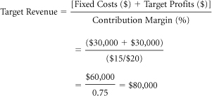
Data Sources, Complications, and Cautions
The information needed to perform a target volume calculation is essentially the same as that required for break-even analysis—fixed costs, selling price, and variable costs. Of course, before determining target volume, one must also set a profit target.
The major assumption here is the same as in break-even analysis: Costs are linear with respect to unit volume over the range explored in the calculation.
Related Metrics and Concepts
Target Volumes not based on Target Profit: In this section, we have assumed that a firm starts with a profit target and seeks to determine the volume required to meet it. In certain instances, however, a firm might set a volume target for reasons other than short-term profit. For example, firms sometimes adopt top-line growth as a goal. Please do not confuse this use of target volume with the profit-based target volumes calculated in this section.
Returns and Targets: Companies often set hurdle rates for return on sales and return on investment and require that projections achieve these before any plan can be approved. Given these targets, we can calculate the sales volume required for the necessary return. (See Section 10.2 for more details.)
EXAMPLE: Niesha runs business development at Gird, a company that has established a return on sales target of 15%. That is, Gird requires that all programs generate profits equivalent to 15% of sales revenues. Niesha is evaluating a program that will add $1,000,000 to fixed costs. Under this program, each unit of product will be sold for $100 and will generate a contribution margin of 25%. To reach break-even on this program, Gird must sell $1,000,000/$25 = 40,000 units of product. How much must Gird sell to reach its target return on sales (ROS) of 15%?
To determine the revenue level required to achieve a 15% ROS, Niesha can use either a spreadsheet model and trial and error, or the following formula:

Thus, Gird will achieve its 15% ROS target if it generates $10,000,000 in sales. At a selling price of $100 per unit, this is equivalent to unit sales of 100,000.