Chapter 23 Optical Methods in Solid Mechanics

Optical methods are finding increasing acceptance in the field of experimental solid mechanics due to the easy availability of novel, compact, and sensitive light sources; detectors; and optical components. This, coupled with the faster data and image acquisition, processing, and display has resulted in optical methods providing information directly relevant to engineers in the form they require. The various methods discussed in the earlier chapters provide a background for the methods described in this chapter. Optical methods principally rely on theories of geometric optics or wave optics to gather information on the deformation, strain, and stress distribution in specimen subject to external loads. Methods based on geometric optics such as moiré and speckle correlation usually have simpler optical systems making them more robust at the expense of resolution. Wave optics based systems are generally very sensitive and hence have a more complex optical system.

In this chapter, after a brief introduction to basic solid mechanics, four techniques are discussed—the digital image correlation method, the optical diffraction strain sensor (ODSS), the low birefringence polarimeter, and the digital holographic system. Each has its own niche in application, which is highlighted in this chapter.

23.2 BASIC SOLID MECHANICS

Solid mechanics [1] deals with the action of external forces on deformable bodies. Consider a generic element inside a body subject to external forces as shown in Figure 23.1a. Without loss of generalization, a two-dimensional element is considered and the resulting stresses on this element in the x and y directions are shown in Figure 23.1b. The stresses, two normal stresses (σ_x and σ_y) and the shear stress (τ_xy) can be transformed to a different coordinate system through the stress transformation system or the Mohr’s circle shown in Figure 23.1c. The maximum and minimum normal stresses are the principal stresses (σ₁, σ₂) while the maximum shear stress (τ_max) is at an angle of 45° with the maximum principal stresses. These stresses give rise to strains following the stress–strain equations which are linear for an elastic material. The strains are related to displacement using strain–displacement equations as shown in Figure 23.1d. The normal strain along the x-direction, defined as the change in length divided by the original length can be written as ε_x = du/dx, where dx is the length of the original line segment along the x-direction. Similarly, the normal strain in the y-direction is ε_y = du/dy, where dv is the change in the length of the segment whose initial length in the y-direction is dy. The shear strain is the difference between the right angle before deformation and the angle between the line segments after deformation. As with stresses, a Mohr circle of strain can be drawn and the principal strains and maximum shear strains can be determined.

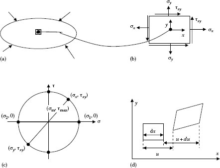
FIGURE 23.1 (a) External forces acting on an object, (b) stress components at a generic point, (c) Mohr’s circle for stress, and (d) strain–displacement relationship.

23.3 DIGITAL IMAGE CORRELATION AND ITS APPLICATIONS

23.3.1 PRINCIPLES OF 2D DIGITAL IMAGE CORRELATION

Two-dimensional digital image correlation (2D DIC) directly provides the full-field in-plane displacement of the test planar specimen surface by comparing the digital images of the planar specimen surface acquired before and after deformation. The strain field can be deduced from the displacement field by numerical differentiation. The basic principle of DIC is schematically illustrated in Figure 23.2. A square reference subset of (2M + 1) × (2M + 1) pixels centered on the point of interest P(x₀, y₀) from the reference image is chosen and its corresponding location in the deformed image determined through a cross-correlation or sum-squared difference correlation criterion. The peak position of the distribution of correlation coefficients determines the location of P(x₀, y₀) in the deformed image, which yields the in-plane displacement components, u and v at point (x₀, y₀). The displacements can similarly be computed at each point on the user-defined grid to obtain the full-field deformation fields.

Following the compatibility of deformation, Q(x, y) around the subset center P(x₀, y₀) in the reference, subset can be mapped to point Q′(x′, y′) in the target subset according to the following first-order shape function:

$\begin{matrix} x^{'} & = x_{0} + Δ x + u + u_{x} Δ x + u_{y} Δ y \\ y^{'} & = y_{0} + Δ y + v + v_{x} Δ x + v_{y} Δ y \end{matrix}$ $\begin{matrix} x^{'} & = x_{0} + Δ x + u + u_{x} Δ x + u_{y} Δ y \\ y^{'} & = y_{0} + Δ y + v + v_{x} Δ x + v_{y} Δ y \end{matrix}$

(23.1)

where

u and v are the displacement components for the subset center P in the x and y directions, respectively

Δx and Δy are the distance from the subset center P to point Q

u_x, u_y, v_x, and v_y are the displacement gradient components for the subset as shown in Figure 23.1

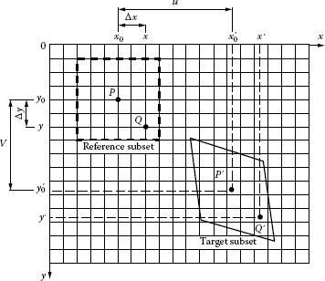
FIGURE 23.2 Schematic figure of digital image correlation method.

To obtain accurate estimation for the displacement components of the same point in the reference and deformed images, the following zero-normalized sum of squared differences correlation criteria [2], which is insensitive to the linear offset and illumination intensity fluctuations, is utilized to evaluate the similarity of reference and target subsets:

$C_{f, g} (p) = \sum_{x = - M}^{M} \sum_{y = - M}^{M} {[\frac{f (x, y) - f_{m}}{\sqrt{\sum_{x = - M}^{M} \sum_{y = - M}^{M} {[f (x, y) - f_{m}]}^{2}}} - \frac{g (x^{'}, y^{'}) - g_{m}}{\sqrt{\sum_{x = - M}^{M} \sum_{y = - M}^{M} {[g (x^{'}, y^{'}) - g_{m}]}^{2}}}]}^{2}$ $C_{f, g} (p) = \sum_{x = - M}^{M} \sum_{y = - M}^{M} {[\frac{f (x, y) - f_{m}}{\sqrt{\sum_{x = - M}^{M} \sum_{y = - M}^{M} {[f (x, y) - f_{m}]}^{2}}} - \frac{g (x^{'}, y^{'}) - g_{m}}{\sqrt{\sum_{x = - M}^{M} \sum_{y = - M}^{M} {[g (x^{'}, y^{'}) - g_{m}]}^{2}}}]}^{2}$

(23.2)

where

f(x, y) is the gray level intensity at coordinates (x, y) in the reference subset of the reference image

g(x′, y′) is the gray level intensity at coordinates (x′, y′) in the target subsets of the deformed image $f_{m} = \frac{1}{{(2 M + 1)}^{2}} \sum_{x = - M}^{M} \sum_{x = - M}^{M} [f (x, y)]$ $f_{m} = \frac{1}{{(2 M + 1)}^{2}} \sum_{x = - M}^{M} \sum_{x = - M}^{M} [f (x, y)]$ and $g_{m} = \frac{1}{{(2 M + 1)}^{2}} \sum_{x = - M}^{M} \sum_{y = - M}^{M} [g (x^{'}, y^{'})]$ $g_{m} = \frac{1}{{(2 M + 1)}^{2}} \sum_{x = - M}^{M} \sum_{y = - M}^{M} [g (x^{'}, y^{'})]$ are the mean intensity values of reference and target subsets, respectively

p = (u, u_x, u_y, v, v_x, v_y)^T denotes the desired vector with respect to six mapping parameters as given in Equation 23.1.

Equation 23.2 can be optimized to get the desired displacement components in the x and y directions using the Newton–Raphson iteration method. A least square smoothing of the computed displacement field provides the required information for strain calculation.

23.3.2 PRINCIPLES OF 3D DIGITAL IMAGE CORRELATION

The 3D DIC technique is based on a combination of the binocular stereo vision technique and the conventional 2D DIC technique. Figure 23.3 is a schematic illustration of the basic principle of the binocular stereo vision technique where O_c1 and O_c2 are optical centers of the left and right cameras, respectively. It can be seen from the figure that a physical point P is imaged as point P₁ in the image plane of the left camera and point P₂ in the image plane of the right camera. The 3D DIC technique aims to accurately recover the 3D coordinates of point P with respect to a world coordinate system from points P₁ and P₂.

To determine the 3D coordinates of point P, there is a need to establish a world coordinate system, which can be accomplished by a camera calibration technique. The world coordinate system is the one on which the final 3D shape reconstruction will be based. The second step is to calculate the location disparities of the same physical point on the object surface from the two images. Based on the calibrated parameters of the two cameras and the measured disparities of the point, the 3D coordinates of point P can then be determined.

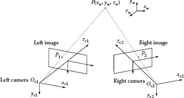
FIGURE 23.3 Schematic diagram of the binocular stereovision measurement.

Camera calibration is the procedure to determine the intrinsic parameters (e.g., effective focal length, principle point, and lens distortion coefficient) and extrinsic parameters (including the 3D position and orientation of the camera relative to a world coordinate system) of a camera. For the 3D DIC technique, the calibration also involves determining the relative 3D position and orientation between the two cameras. As the accuracy of the final measurement heavily depends on the obtained calibration parameters, camera calibration plays an important role in the 3D DIC measurement.

The goal of the stereo matching is to precisely match the same physical point in the two images captured by the left and right cameras. This task, commonly considered the most difficult part in stereovision measurement, can be accomplished by using the well-established subset-based matching algorithm adopted in the 2D DIC technique. The basic concept of the 2D DIC technique is to match the same physical point from two images captured before and after deformation (only one camera is employed, and is fixed during measurements); to ensure a successful and accurate matching, the specimen surface is usually coated with random speckle patterns. Similar to but slightly different from the 2D DIC scheme, the stereo matching used in the 3D DIC technique aims to match two random speckle patterns on specimen surface recorded by the left and right cameras [3].

Based on the obtained calibration parameters of each camera and the calculated disparities of points in the images, the 3D world coordinates of the points in the regions of interest on the specimen surface can be easily determined using the classical triangulation method. By tracking the coordinates of the same physical points before and after deformation, the 3D motions of the each point can be determined. Similarly, the same technique proposed in previous section can be utilized for the strain estimation based on obtained displacement fields.

23.3.3 APPLICATION TO RESIDUAL STRAIN MEASUREMENT

One specific application of the DIC method for the residual plastic deformation of a notched specimen under fatigue test is exemplified to show the capability of the method. A tensile specimen with semicircular notch in the middle as shown in Figure 23.4 is used as the test specimen.

Figure 23.5 shows the surface displacement fields computed using the Newton–Rapshon method after 26,000 fatigue cycles. It is seen that the displacement in x-direction (normal to the loading direction) is much smaller than that of y-direction. Figure 23.6 shows the residual plastic strain distributions computed from the displacement field using a point-wise least squares fitting technique.

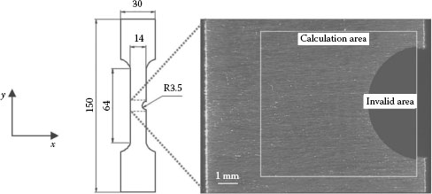
FIGURE 23.4 Geometry of the specimen. The region of interest and the invalid area is highlighted.

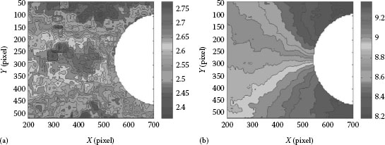
FIGURE 23.5 Residual displacement fields of the specimen surface after 26,000 fatigue cycles: (a) u displacement field and (b) v displacement field.

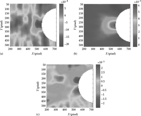
FIGURE 23.6 The residual plastic strain fields derived from the displacement field: (a) ε_x, (b) ε_y, and (c) γ_xy.

23.4 LOW BIREFRINGENCE POLARISCOPE

A modified Senarmont polariscope coupled to a phase-shift image-processing system provides a system for measurement of low levels of birefringence. The birefringence is related to the change in phase between the two propagating polarized waves through the specimen and can be related to the principle stress difference. In addition, the difference in the normal stress and the shear stress distribution can be quantitatively determined.

23.4.1 PRINCIPLE OF LOW BIREFRINGENCE POLARISCOPE

In the current system, schematically shown in Figure 23.7, the specimen is illuminated with circularly polarized light. The birefringence in the specimen transforms the circular polarized light to one with elliptic polarization, which is then interrogated by a rotating linear analyzer.

The change in polarization by the specimen can be attributed to a change in the orientation of the fast axis of the light as well as a phase lag between the two polarization components of the input beam. For materials, where the birefringence is attributed to the stress, the change in orientation of the fast axis (β) is related to the direction of the principal stresses while the phase lag (Δ) is related to the principal stress difference as

$Δ = \frac{2 π C d}{λ} = (σ_{1} - σ_{2})$ $Δ = \frac{2 π C d}{λ} = (σ_{1} - σ_{2})$

(23.3)

where

d is the material thickness

λ is the wavelength of light

C is the stress optic coefficient of the material

σ₁ and σ₂ are the principal stresses

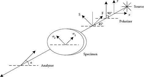
FIGURE 23.7 Optical train for a low birefringence polariscope.

From Jones’ calculus, the components of the transmitted light vector perpendicular and parallel to the analyzer axis (U, V) are

$[\begin{matrix} U \\ V \end{matrix}] = J_{A} J_{M} J_{Q} J_{P} a e^{j ω t}$ $[\begin{matrix} U \\ V \end{matrix}] = J_{A} J_{M} J_{Q} J_{P} a e^{j ω t}$

(23.4)

where J_P J_q, J_M, and J_A are the Jones’ vector for the polarizer, the quarter-wave plate (QWP), the model, and the analyzer respectively. Expanding using matrix multiplication gives

$\begin{array}{l} {\begin{matrix} U \\ V \end{matrix}} & = \frac{\sqrt{2}}{2} [\begin{matrix} 0 & 0 \\ \cos α & \sin α \end{matrix}] [\begin{matrix} \cos Δ / 2 - i \cos 2 β sin Δ / 2 & - i \sin 2 β sin Δ / 2 \\ - i \sin 2 β sin Δ / 2 & \cos Δ / 2 + i \cos 2 β sin Δ / 2 \end{matrix}] \times [\begin{matrix} 1 & i \\ i & 1 \end{matrix}] [\begin{matrix} 0 \\ 1 \end{matrix}] a e^{j ω t} \\ = \frac{\sqrt{2}}{2} [(\sin \frac{Δ}{2} \cos (α - 2 β) + \sin α cos \frac{Δ}{2}) + i (\sin \frac{Δ}{2} \sin (α - 2 β) + \cos α cos \frac{Δ}{2})] a e^{j ω t} \end{array}$ $\begin{array}{l} {\begin{matrix} U \\ V \end{matrix}} & = \frac{\sqrt{2}}{2} [\begin{matrix} 0 & 0 \\ \cos α & \sin α \end{matrix}] [\begin{matrix} \cos Δ / 2 - i \cos 2 β sin Δ / 2 & - i \sin 2 β sin Δ / 2 \\ - i \sin 2 β sin Δ / 2 & \cos Δ / 2 + i \cos 2 β sin Δ / 2 \end{matrix}] \times [\begin{matrix} 1 & i \\ i & 1 \end{matrix}] [\begin{matrix} 0 \\ 1 \end{matrix}] a e^{j ω t} \\ = \frac{\sqrt{2}}{2} [(\sin \frac{Δ}{2} \cos (α - 2 β) + \sin α cos \frac{Δ}{2}) + i (\sin \frac{Δ}{2} \sin (α - 2 β) + \cos α cos \frac{Δ}{2})] a e^{j ω t} \end{array}$

(23.5)

where

α is the angular position of the rotating polarizer

β is the orientation of the fast axis (maximum principal stress direction)

a is the amplitude of the circularly polarized light

ω is the temporal angular frequency of the wave

The intensity of light emerging from a point on the specimen is then given as

$I = {| V |}^{2} = \frac{a^{2}}{2} [1 + \sin Δ \sin 2 (α - β)]$ $I = {| V |}^{2} = \frac{a^{2}}{2} [1 + \sin Δ \sin 2 (α - β)]$

(23.6)

As the analyzer transmission axis aligns with the maximum intensity axis twice per full rotation, the intensity will be modulated at 2α intervals with a phase of 2β. Equation 23.6, the intensity collected by the detector, can be rewritten as

$I = I_{a} + I_{cα} \cos 2 α + I_{sα} \sin 2 α$ $I = I_{a} + I_{cα} \cos 2 α + I_{sα} \sin 2 α$

(23.7)

where

$\begin{array}{l} I_{cα} & = - [\frac{a^{2}}{2} \sin Δ] \sin 2 β \\ I_{sα} & = (\frac{a^{2}}{2} \sin Δ) \cos 2 β \end{array}$ $\begin{array}{l} I_{cα} & = - [\frac{a^{2}}{2} \sin Δ] \sin 2 β \\ I_{sα} & = (\frac{a^{2}}{2} \sin Δ) \cos 2 β \end{array}$

I_a = a²/2, which is the average light intensity collected by the detector unit.

23.4.2 FOUR-STEP PHASE-SHIFTING METHOD

In order to determine the phase lag (Δ) and the direction of the fast axis (β) from Equation 23.6, we need at least three more equations. These are obtained by recording phase-shift patterns by changing the angle (α) of the analyzer. Assuming the average light intensity I_a to be constant at a given point during experiment, a four-step phase-shifting method can be used. Table 23.1 summarizes the four optical arrangements and the corresponding intensity equations.

TABLE 23.1
Intensity Equations for Rotating Analyzer Method

Number	Analyzer Angle α	Intensity Equation
1	0	I₁ = I_a (1 − sin Δ sin 2β)
2	π/4	I₂ = I_a (1 + sin Δ cos 2β)
3	π/2	I₃ = I_a (1 + sin Δ sin 2β)
4	3π/4	I₄ = I_a (1 − sin Δ cos 2β)

The retardation and direction of the fast axis can be deduced as

$Δ = \frac{1}{2 I_{a}} {[{(I_{3} - I_{1})}^{2} + {(I_{4} - I_{2})}^{2}]}^{1 / 2}$ $Δ = \frac{1}{2 I_{a}} {[{(I_{3} - I_{1})}^{2} + {(I_{4} - I_{2})}^{2}]}^{1 / 2}$

(23.8a)

$β = \frac{1}{2} \tan^{- 1} (\frac{I_{1} - I_{3}}{I_{4} - I_{2}})$ $β = \frac{1}{2} \tan^{- 1} (\frac{I_{1} - I_{3}}{I_{4} - I_{2}})$

(23.8b)

From these values, I_cα and I_sα can be calculated through Equation 23.6. From the Mohr’s circle, it can be seen that the sine and cosine components of the light intensity are directly related to the stresses along the 0°/90° and ±45° planes. Thus,

$\begin{array}{l} I_{sα} \propto (σ_{x x} - σ_{y y}) \\ I_{cα} \propto τ_{x y} \end{array}$ $\begin{array}{l} I_{sα} \propto (σ_{x x} - σ_{y y}) \\ I_{cα} \propto τ_{x y} \end{array}$

(23.9)

23.4.3 LOW BIREFRINGENCE POLARISCOPE BASED ON LIQUID CRYSTAL POLARIZATION ROTATOR

In the above polariscope, there is a need to manually rotate the analyzer, which makes it difficult to achieve high stability and repeatability. A new method based on a liquid crystal polarization rotator to get full-field sub-fringe stress distribution is proposed. By changing the applied voltage to the liquid crystal phase plate, the phase-shift images are recorded and processed to get the stress distribution. Figure 23.8 is the schematic of the proposed polariscope using the liquid crystal (LC) polarization rotator as the phase-shifting element. The LC polarization rotator, a key component of the proposed polariscope system, consists of an LC phase plate inserted between two crossed QWPs. The extraordinary (fast) axis of the first QWP is parallel to the x-axis. The extraordinary axis of the LC phase plate is oriented at 45°, and the extraordinary axis of the second QWP is oriented parallel to the y-axis. An LED light source illuminates the object with circularly polarized light and the transmitted light goes through LC polarization rotator before impinging on the analyzer whose orientation is set parallel to the x-axis (α = 0°).

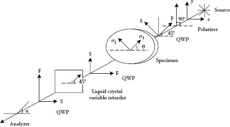
FIGURE 23.8 Schematic of the LC polarization rotator-based polariscope.

Using Jones’ calculus, the components of the transmitted light vector perpendicular to and parallel to the analyzer axis are

$[\begin{matrix} U \\ V \end{matrix}] = J_{A} J_{LC} J_{M} J_{Q} J_{P} a e^{j ω t}$ $[\begin{matrix} U \\ V \end{matrix}] = J_{A} J_{LC} J_{M} J_{Q} J_{P} a e^{j ω t}$

(23.10)

where J_P, J_Q, J_M, J_LC, and J_A are the Jones’ vector for the polarizer, the QWP, the model, the LC polarization rotator, and the analyzer, respectively. Expanding and multiplying the equation

$\begin{array}{l} {\begin{matrix} U \\ V \end{matrix}} = & \frac{\sqrt{2}}{2} [\begin{matrix} 0 & 0 \\ 1 & 0 \end{matrix}] [\begin{matrix} \cos (ϕ / 2) & \sin (ϕ / 2) \\ - \sin (ϕ / 2) & \cos (ϕ / 2) \end{matrix}] \\ \times [\begin{matrix} \cos Δ / 2 + i \cos 2 β sin Δ / 2 & i \sin 2 β sin Δ / 2 \\ i \sin 2 β sin Δ / 2 & \cos Δ / 2 - i \cos 2 β sin Δ / 2 \end{matrix}] [\begin{matrix} 1 & i \\ i & 1 \end{matrix}] [\begin{matrix} 0 \\ 1 \end{matrix}] a e^{i ω t} \end{array}$ $\begin{array}{l} {\begin{matrix} U \\ V \end{matrix}} = & \frac{\sqrt{2}}{2} [\begin{matrix} 0 & 0 \\ 1 & 0 \end{matrix}] [\begin{matrix} \cos (ϕ / 2) & \sin (ϕ / 2) \\ - \sin (ϕ / 2) & \cos (ϕ / 2) \end{matrix}] \\ \times [\begin{matrix} \cos Δ / 2 + i \cos 2 β sin Δ / 2 & i \sin 2 β sin Δ / 2 \\ i \sin 2 β sin Δ / 2 & \cos Δ / 2 - i \cos 2 β sin Δ / 2 \end{matrix}] [\begin{matrix} 1 & i \\ i & 1 \end{matrix}] [\begin{matrix} 0 \\ 1 \end{matrix}] a e^{i ω t} \end{array}$

(23.11)

The intensity of light emerging from a point on the specimen is thus

$I = {| V |}^{2} = \frac{a^{2}}{2} [1 + \sin Δ \sin (δ - 2 β)]$ $I = {| V |}^{2} = \frac{a^{2}}{2} [1 + \sin Δ \sin (δ - 2 β)]$

(23.12)

Table 23.2 summarizes the four optical arrangements and the corresponding intensity equations.

It can be seen that the intensity equations are the same as those of Table 23.1. In this case, the phase retardation is due to changes in voltage applied to the liquid crystal rather than rotation of the analyzer. This can be electronically controlled resulting in much better precision and accuracy for the phase-shift routine.

TABLE 23.2
Intensity Equations Used in the New Method

Number	Phase Retardation 8	Intensity Equation
1	0	I₁ = I_a (1 − sin Δ sin 2β)
2	π/2	I₂ = I_a (1 + sin Δ cos 2β)
3	π	I₃ = I_a (1 + sin Δ sin 2β)
4	3π/2	I₄ = I_a (1 − sin Δ cos 2β)

23.4.4 EXPERIMENTAL RESULTS

An epoxy disc (22 mm diameter and 3 mm thick) under diameteral compression of a load of 0.98 kg is tested because of its well-known principal stress magnitude and direction. Both polariscopes were tested and the images processed using a MATLAB® algorithm [4] to determine the desired phase lag and orientation of the fast axis. The experimental results using the low birefringence polariscope and the polariscope based on liquid crystal polarization rotator are shown in the left images of Figure 23.9 whereas the images on the right were obtained using the rotating analyzer method. The normal stress difference map is symmetric as shown in Figure 23.9c while the shear stress is antisymmetric (Figure 23.9d) about both the x and y axes as expected. These stress distributions also match with theory and show the high sensitivity of the system.

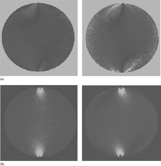
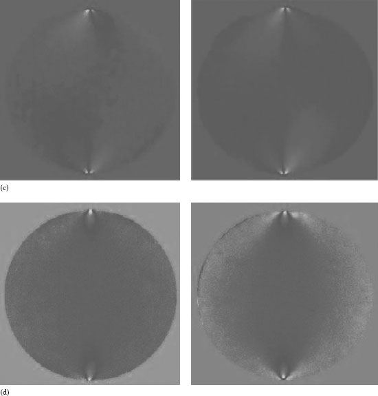
FIGURE 23.9 Experimental results using LC polarization rotator (left) and rotating the analyzer (right). (a) Direction map and (b) phase map. Experimental results using LC polarization rotator (left) and rotating the analyzer (right). (c) σ₊₄₅−σ_–45 and (d) σ_x-σ_y.

23.5 OPTICAL DIFFRACTION STRAIN SENSOR

23.5.1 PRINCIPLE OF THE OPTICAL DIFFRACTION STRAIN SENSOR

The basic principle of measurement is illustrated in Figure 23.10. A diffraction grating bonded to the surface of the specimen follows the deformation of the underlying specimen. Consider a thin monochromatic collimated beam that is normal to the grating plane and illuminating a point on a specimen grating. The diffraction is governed by the equation:

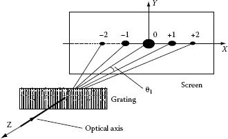
$\begin{matrix} p \sin θ = n λ & n = 0, \pm 1, \pm 2, \pm 3, \dots \end{matrix}$ $\begin{matrix} p \sin θ = n λ & n = 0, \pm 1, \pm 2, \pm 3, \dots \end{matrix}$

(23.13)

FIGURE 23.10 Sketch of one-dimensional grating diffraction. Grating is illuminated by a collimated beam; a line of diffraction spots is formed on a screen.

where

p is the grating pitch

n is the diffraction order

λ is the light wavelength

θ is the diffraction angle

When the specimen and hence the grating deforms, the pitch changes to p*, with a corresponding change in θ according to Equation 23.1. Thus, the strain along the x-direction at the illuminated point on the grating can be determined as

$ε_{x} = \frac{p * - p}{p} = \frac{X_{n}^{*} - X_{n}}{X_{n}} \cos θ_{n}$ $ε_{x} = \frac{p * - p}{p} = \frac{X_{n}^{*} - X_{n}}{X_{n}} \cos θ_{n}$

(23.14)

where X_n and $X_{n}^{*}$ $X_{n}^{*}$ are the centroids of the undeformed and deformed nth-order diffraction spot. These centroids can be determined precisely with subpixel accuracy. If a cross grating is used instead of a line grating, the strain along y-direction, ε_y can be similarly obtained. The shear strain γ_xy can also be evaluated.

By using a high-frequency grating and a sensitive position-sensing detector, a system with capabilities to rival the electrical resistance strain gauge has been developed [5]. The schematic of the setup and typical result of strain distribution along the interface of the die and substrate in an electronic package is shown in Figure 23.11. The display interface directly determines the strain at a particular point and since the diffraction grating can cover a large area, strains at different points can be monitored by translating the specimen. Furthermore, the gauge length that is determined by the size of the laser beam can be readily adjusted and the system has been demonstrated for dynamic strain measurement. Overall, it is a worthy challenger for the electrical strain gauge.

23.5.2 MULTIPOINT DIFFRACTION STRAIN SENSOR

The patented multipoint diffraction strain sensor (MISS) [6] uses a high-frequency diffraction grating along with a micro-lens array-based CCD detector. A reflective diffraction grating is bonded to the surface of the specimen and follows the deformation of the underlying specimen. The grating is illuminated by two symmetric monochromatic laser beams at a prescribed angle such that the first-order diffracted beams emerge normal to the specimen surface. The micro-lens array samples each of the incident beams and focuses them as spots onto the CCD as shown in Figure 23.12a. When the specimen is deformed, tilted, or rotated, the diffracted wave fronts emerging from the specimen are distorted and hence the spots shift accordingly. Figure 23.12b shows the simulated spot pattern for a 4 × 4 array of micro-lenses for one of the beams when the specimen is unstrained, undergoes uniform strain and nonuniform strain. The symmetric beam incident from other direction gives a similar array of spot patterns. Strains at each spot location which corresponds to a small area of the specimen, can then be readily deduced from the shift of the spots as described below. Without loss of generality, spots shifts in a single direction are used in this derivation.

FIGURE 23.11 (a) Schematic of the ODSS and (b) strain distribution along the interface of die and substrate of an electronic package.

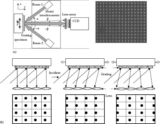
FIGURE 23.12 (a) Schematic of MISS with spot image from the two sources and (b) shift in spots due to uniform and nonuniform strain.

Starting from the well-known diffraction equation, the change in diffraction angle when the specimen is subject to strain, ε_x, and out-of-plane tilt, Δϕ, can be deduced. Hence the corresponding shift, Δx, of a typical spot on the CCD plane can be related to the strain and tilt as

$\begin{array}{l} \frac{K_{f} Δ x_{1}}{f} & = - ε_{x} f \sin α + Δ ϕ (1 + \cos α) \\ \frac{K_{f} Δ x_{2}}{f} & = + ε_{2} f \sin α + Δ ϕ (1 + \cos α) \end{array}$ $\begin{array}{l} \frac{K_{f} Δ x_{1}}{f} & = - ε_{x} f \sin α + Δ ϕ (1 + \cos α) \\ \frac{K_{f} Δ x_{2}}{f} & = + ε_{2} f \sin α + Δ ϕ (1 + \cos α) \end{array}$

(23.15)

where

f is the focal length of each micro-lens

α is the angle of incidence

K_f is a multiplication factor which is 1 if the two beams are collimated and the subscripts 1 and 2 refer to the two incident beams

Solving Equation 23.15

$ε_{x} = K_{f} \frac{Δ x_{2} - Δ x_{1}}{2 f \sin α}$ $ε_{x} = K_{f} \frac{Δ x_{2} - Δ x_{1}}{2 f \sin α}$

(23.16a)

$Δ ϕ = K_{f} \frac{Δ x_{2} + Δ x_{1}}{2 f (1 + \cos α)}$ $Δ ϕ = K_{f} \frac{Δ x_{2} + Δ x_{1}}{2 f (1 + \cos α)}$

(23.16b)

The two incident beams thus enable us to compute the strains and the rigid body tilts of the specimen separately.

Figure 23.13a shows the uniform strain on specimen; note that the shear or rotation component that causes the spots to shift in the perpendicular direction is nearly zero. Similarly, for a specimen subject to pure rotation, the normal component of strain is zero as shown in Figure 23.13b.

23.6 DIGITAL HOLOGRAPHY

23.6.1 INTRODUCTION

In digital holography, the optical hologram is digitally recorded by CCD or CMOS arrays. It is then reconstructed numerically to determine the amplitude and phase of the object beam. The amplitude provides the intensity image while the phase provides the optical path difference between the object and reference beam. This quantitative measurement of phase is one of the key aspects of the digital holographic system leading to its widespread adoption in a variety of applications.

23.6.2 REFLECTION DIGITAL HOLOGRAPHY

Reflection digital holography [7] is widely used for deformation and shape measurement. The schematic of the reflection holographic setup is shown in Figure 23.14. Collimated light from a laser is split into two beams—the object beam which scatters of the object, and a reference beam.

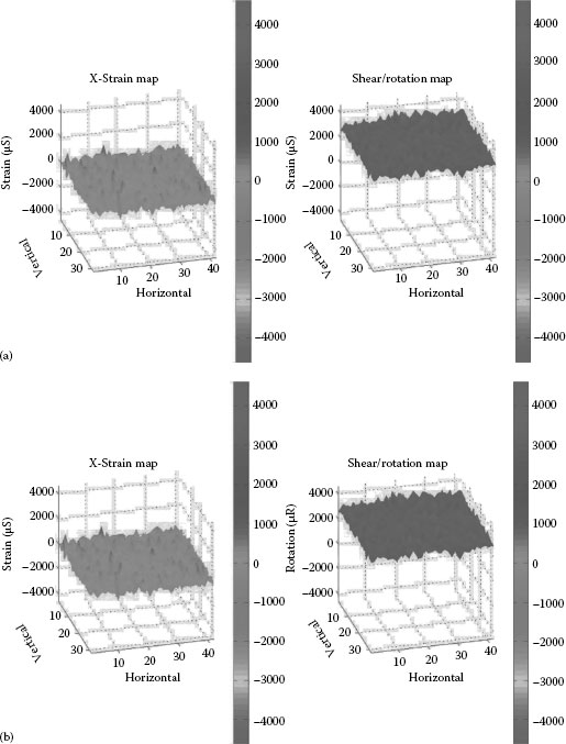
FIGURE 23.13 (a) 2D strain map of specimen subject to uniform strain and (b) 2D strain map of specimen subject to pure rotation.

The reference mirror can be tilted to create an off-axis holographic recording. However, due to the low resolution of the digital camera, the angle needs to satisfy the sampling theorem in order to record the hologram. Alternatively, an in-line setup can also be used. However, in this case, the effect of the zero order and twin image needs to be accounted for. This can readily be done through software [5].

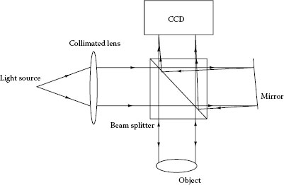
FIGURE 23.14 Schematic of the reflection digital holographic.

The numerical reconstruction of the digital hologram is actually a numerical simulation of the scalar diffraction. Usually, two methods, the Fresnel transform method and the convolution method, are used. Numerical reconstruction by the Fresnel transform method requires simulation of the following equation:

$U (n Δ x_{i}, m Δ y_{i}) = e^{jπdλ (\frac{n^{2}}{N^{2} Δ x_{h}^{2}} + \frac{m^{2}}{M^{2} Δ y_{h}^{2}})} \sum_{k = 0}^{N - 1} \sum_{l = 0}^{M - 1} h (k Δ x_{h}, l Δ y_{h}) R * (k Δ x_{h}, l Δ y_{h}) e^{\frac{j π}{dλ} (k^{2} Δ x_{h}^{2} + l^{2} Δ y_{h}^{2})} e^{- 2 j π (\frac{k n}{N} + \frac{l m}{M})}$ $U (n Δ x_{i}, m Δ y_{i}) = e^{jπdλ (\frac{n^{2}}{N^{2} Δ x_{h}^{2}} + \frac{m^{2}}{M^{2} Δ y_{h}^{2}})} \sum_{k = 0}^{N - 1} \sum_{l = 0}^{M - 1} h (k Δ x_{h}, l Δ y_{h}) R * (k Δ x_{h}, l Δ y_{h}) e^{\frac{j π}{dλ} (k^{2} Δ x_{h}^{2} + l^{2} Δ y_{h}^{2})} e^{- 2 j π (\frac{k n}{N} + \frac{l m}{M})}$

(23.17)

where

$Δ x_{i} = \frac{d λ}{N Δ x_{h}}$ $Δ x_{i} = \frac{d λ}{N Δ x_{h}}$ and $Δ y_{i} = \frac{d λ}{M Δ y_{h}}$ $Δ y_{i} = \frac{d λ}{M Δ y_{h}}$ are the pixel sizes in the reconstructed image plane

h(kΔx_h, lΔy_h) is the hologram

R* (kΔx_h, lΔy_h) is the reference beam

Numerical reconstruction by the convolution method gives a reconstruction formula of digital holography as follows:

${\begin{array}{l} U (n Δ x_{i}, m Δ y_{i}) = F^{- 1} {F [h (k Δ x_{h}, l Δ y_{h}) R * (k Δ x_{h}, l Δ y_{h})] \cdot G (n Δ ξ, m Δ η)} \\ G (n Δ ξ, m Δ η) = e^{\frac{2 jπ d}{λ} \sqrt{1 - {[\frac{λ (n - 1)}{N Δ ξ}]}^{2} - {[\frac{λ (m - 1)}{M Δ η}]}^{2}}} \end{array}$ ${\begin{array}{l} U (n Δ x_{i}, m Δ y_{i}) = F^{- 1} {F [h (k Δ x_{h}, l Δ y_{h}) R * (k Δ x_{h}, l Δ y_{h})] \cdot G (n Δ ξ, m Δ η)} \\ G (n Δ ξ, m Δ η) = e^{\frac{2 jπ d}{λ} \sqrt{1 - {[\frac{λ (n - 1)}{N Δ ξ}]}^{2} - {[\frac{λ (m - 1)}{M Δ η}]}^{2}}} \end{array}$

(23.18)

where

h(kΔx_h, lΔy_h) is the hologram

R* (kΔx_h, lΔy_h) is the reference beam

G(nΔξ, mΔη) is the optical transfer function in the frequency domain

Δx_h, Δy_h are the pixel sizes in the hologram plane

Δξ, Δη are the pixel sizes in the frequency domain

Δx_i, Δy_i are the pixel sizes in the image plane

Using Fresnel transform method, the resolution of the reconstructed object wave depends not only on the wavelength of the illuminating light but also on the reconstruction distance and it is always lower than the resolution of the CCD camera. While using the convolution method, one can obtain the reconstructed object wave with the maximum resolution with the same pixel size as that of the CCD camera.

The reconstruction by convolution method is shown in Figure 23.15 where Figure 23.15a is the recorded hologram, and Figure 23.15b is the Fourier transform of the hologram showing the zero order and the two other orders corresponding to the object wave. One of these orders is isolated and moved to the origin to remove the tilt due to the reference beam. It is then multiplied by the transfer function and propagated to the image plane. An inverse Fourier transform of the product gives the reconstructed object wave from which the quantitative amplitude (Figure 23.15c) and phase (Figure 23.15d) can be extracted.

The phase, φ(x, y) which is related to the optical path difference between the object and reference waves can thus be used to obtain the height, d(x, y, z) of the object as

$φ (x, y) = \frac{2 π}{λ} d (x, y, z)$ $φ (x, y) = \frac{2 π}{λ} d (x, y, z)$

(23.19)

If the phase is −π < φ(x, y) < π, the height can be directly determined without the need to unwrap the data. This corresponds to a height between ±λ/2. With an 8 bit resolution CCD camera and a 532 nm frequency-doubled diode-pumped laser, this results in a sensitivity of about 2 nm. If, however, the phase exceeds this value, then, unwrapping becomes necessary to extract the true height distribution.

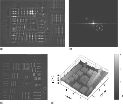
FIGURE 23.15 (a) Digital hologram of USAF positive target, (b) spectra, (c) intensity, and (d) quantitative 3D phase map.

23.6.3 DIGITAL HOLOGRAPHIC INTERFEROMETRY

Digital holographic interferometry proceeds in much the same way as traditional holographic interferometry as far as recording is concerned. In the reconstruction step, the phases of the holograms before and after deformation are extracted and subtracted to reveal the modulo 2π fringes. These can be readily unwrapped to reveal the true deformation [8]. In previous cases, magnifying optics was necessary to enlarge the object and increase its spatial resolution. In this approach, a patented [9] system based on the same Michelson interferometer geometry, as shown in Figure 23.14, was adopted. However, instead of a collimated beam, a diverging beam was used as shown in Figure 23.16a. The setup in this configuration can be quite compact and still provide the desired magnification. The reconstruction process is slightly different since the reference beam is not collimated and hence the appropriate divergence of the beam has to be incorporated into the reconstruction equations. A typical reconstruction of 300 μm long and 20 μm wide micro-cantilevers using this setup is shown in Figure 23.16b, which can be readily compared to a microscope image shown in Figure 23.16c.

In holographic interferometry, there are two possibilities—for static deformation measurement, the double exposure method is used. In this, two digital holograms of the object before and after deformation are recorded. They are separately reconstructed and their phase extracted. The phase difference provides the deformation of the object between the two exposures. A MEMS microheater was chosen as the sample. Two exposures before and after application of a current, which caused the micro-heaters to deform, were recorded. The resulting out of displacements of the microheater is shown in Figure 23.17a. Alternately, if the cantilevers were subject to dynamic loading, a time average hologram, where the exposure time is greater than the period of vibration, is recorded. Reconstruction of this hologram reveals the familiar Bessel-type fringes modulating the amplitude image as shown in Figure 23.17b. The excitation frequency was 417 kHz.

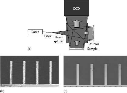
FIGURE 23.16 (a) Schematic of lensless microscopic digital holographic interferometer.

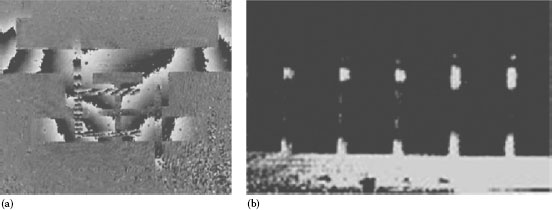
FIGURE 23.17 (a) Double exposure lensless microscopic digital holographic interferometery of MEMS micro-heater; and (b) time average digital holographic interferometry of cantilever vibrating at 417 kHz.

23.7 CONCLUSIONS

Optical methods in solid mechanics have shown tremendous growth in the past decade. With the availability of novel light sources and detectors and faster data acquisition and processing speeds, real-time deformation and strain measurement is now possible. In this chapter, four different approaches have been demonstrated for deformation and strain measurement. The digital correlation method appears to be a simple and straightforward method for deformation and strain measurement. However, the strain sensitivity of ~100 με leaves a bit to be desired. Despite this, there are various applications for which this method would be particularly suited. The polariscope system requires transparent birefringent material. This limits its application but with increasing use of polymers, plastics, and glasses, measuring low levels of birefringence becomes particularly relevant and the low birefringence polariscope has significant applications. With the use of an infrared light source, it would also be possible to extend this to measure residual stress in silicon wafers, which would be of great interest to the semiconductor and MEMS industry. The ODSS has tremendous potential as an alternative to the ubiquitous strain gauge. Its specifications match or surpass that of the traditional strain gauge. With its ability to monitor multiple points at the same time, this has particular interest in whole-field strain analysis without the need for numerical differentiation. Finally, digital holography has shown great promise as a novel tool of nanoscale deformation measurement of micron-sized objects. It has specific applications in the fields of static and dynamic MEMS characterization. However, unlike the other methods, digital holography provides out-of-plane displacements and not directly related to in-plane deformation and stress measurement.

REFERENCES

1. Asundi A. Introduction to engineering mechanics, in P. Rastogi (ed.), Photomechanics, Topics in Applied Physics, Chapter 2, Vol. 77, Springer Verlag, New York, 2000.

2. Pan B, Xie HM, Guo ZQ, and Hua T. Full-field strain measurement using a two-dimensional Savitzky-Golay digital differentiator in digital image correlation, Optical Engineering, 46(3), 033601–1–033601–10, 2007.

3. Luo PF, Chao YJ, and Sutton MA, Accurate measurement of three-dimensional displacement in deformable bodies using computer vision, Experimental Mechanics, 33(2), 123–132, 1993.

4. Asundi A. MATLAB^® for Photomechanics—A Primer, Elsevier Science Ltd., Oxford, U.K., 2002.

5. Zhao B, Xie H, and Asundi A. Optical strain sensor using median density grating foil: Rivaling in electric strain gauge, Review of Scientific Instrument, 72(2), 1554–1558, 2001.

6. Asundi A. Moire interferometric strain sensor, Patent No. TD/006/05, 2005.

7. Asundi A and Singh VR. Circle of holography—Digital in-line holography for imaging, microscopy and measurement, Journal of Holography and Speckle, 3, 106–111, 2006.

8. Xu L, Peng XY, Miao J, and Asundi A. Hybrid holographic microscope for interferometric measurement of microstructures, Optical Engineering, 40(11), 2533–2539, 2001.

9. Asundi A and Singh VR, Lensless digital holographic microscope, Nanyang Technological University, Singapore, Technology Disclosure Number, TD/016/07, 2007.

..................Content has been hidden....................

You can't read the all page of ebook, please click here login for view all page.

Table of Contents for Chapter 23 Optical Methods in Solid Mechanics

Create new playlist

Sign In

Sign Up

Table of Contents for
Chapter 23 Optical Methods in Solid Mechanics