
CONTENTS
22.2.1.1 Single Photogrammetry
22.2.1.2 Stereo Photogrammetry
22.2.1.3 Photogrammetry with Many Images (Bundle Adjustment)
22.2.2 Flow of Measuring Process
22.2.2.5 3D Image Reconstruction and Output
22.2.3 Photogrammetric SLAM (Visual SLAM, SFM)
22.3 Application Examples of 3D Measurement and Modeling
22.3.1 Application of Cultural Heritage, Architecture, and Topography
22.3.1.1 3D Modeling of Wall Relief
22.3.1.2 Byzantine Ruins on Gemiler Island
22.3.1.3 All-Around Modeling of a Sculpture in the Archaeological Museum of Messene in Greece
22.3.1.4 All-Around Modeling of the Church of Agia Samarina
22.3.1.6 3D Model Production with Aerial and Ground Photographs
22.3.2 Application to Human Body Measurement
22.3.3 Application to Automobile Measurement
22.3.3.2 Measuring Surface of the Entire Body
22.3.3.3 Measuring Surface of the Tire
22.3.5.1 Measurement by Vehicle (Measurement by Image Sequences)
22.3.5.2 Measurement by UAV (Measurement by Image Sequences and Still Images)
Recent developments in the digital camera with its extremely dense pixel capacity and that of the PC with its high speed and enormous memory capacity has enabled us to process the super-voluminous data involved in point clouds and photo data for three-dimensional (3D) works, computer graphics, and virtual reality (VR) with very high speed and efficiency. Its applied technology is rapidly expanding not only in mapmaking but also in such new areas as archiving and preserving valuable cultural heritages, forensics, civil engineering, architecture construction, industrial measurement, human body measurement, even to such areas as entertainment animation. And it is daily opening new vistas, as it is integrated with devices like global positioning system (GPS), total station, gyrosensor, accelerometer, laser scanner, and video image [1].
Here, we explain its technological principles and practical applications with our newly developed software for digital photogrammetry (Topcon Image Master, PI-3000) [6,13,23,61].
Photogrammetry technology has developed with aerial photogrammetry for mapmaking and terrestrial photogrammetry, which measures and surveys the ground with metric camera. It has also developed with close-range photogrammetry, which measures large constructions with precision in the industrial measuring [2,3]. Digital photogrammetry, therefore, is the digital photo technology, which replaced film-based data with digital data to integrate with the image-processing technology [4].
The basic principle of photogrammetry [2,3] is based on photo image, center of projection, and the geometrical condition called colinearity condition, where the objects should be on the same straight line (Figure 22.1a). In digital photogrammetry, we have three different types: (1) single photogrammetry with one single photograph, (2) stereo photogrammetry with two photographs as one unit, and (3) photogrammetry with many photographs, using (1) or (2) or their combination. These methods are performed through mathematical calculation and image processing; the basic system structure is composed of nothing other than a PC, a specific software and digital camera.
22.2.1.1 Single Photogrammetry
Figure 22.1a shows the geometry of a single photogrammetry. The light coming from any given point in real space always passes through the projection center (O) and creates image on the photograph. To make 3D measurement of an object with this method, we must satisfy the following conditions other than that of colinearity condition:
1. We must have at least one coordinate of 3D coordinates of the object. For example, in Figure 22.1a, when Z1, which is the coordinate of P1 on Z-axis, is given.
2. The point to be identified should be on the plain or curved surface geometrically. For example, in Figure 22.1a, when P2 is on the specific plane aX + bY + cZ = 0.
Therefore, for measuring or surveying flat plain or topography or flat wall of a building, we use single photogrammetry under these conditions.
The earlier conditions (1) and (2) diminish the number of unknown quantity, because the dimension is diminished from three to two. As a result, the data between two dimensions of the picture and two dimensions of the real space become interchangeable (2D projective transformation).
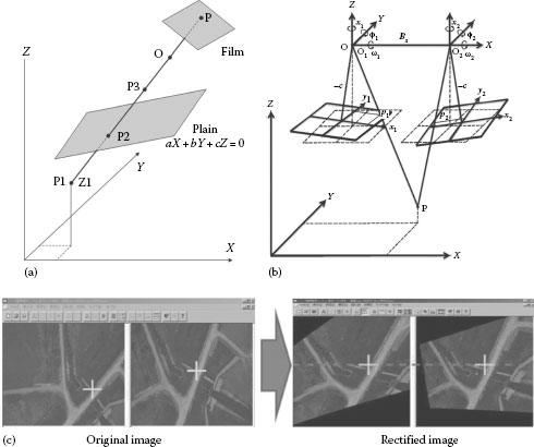
FIGURE 22.1 (a) Single photogrammetry and colinearity condition, (b) stereo method and relative orientation, and (c) rectification.
If we can get more than three control points by which the ground coordinates are measured, we can obtain the exterior orientation parameters (the 3D position of the camera and the inclination of the axes). This process to obtain the position and inclination of the camera from the control points is called “orientation of single photograph” or “space resection.” There is another method called “DLT” method (direct linear transformation), which is also the 3D projective transformation. Though this DLT method requires at least 11 unknown parameters, it is still convenient and simple, because the calculation is done by the linear transformation.
22.2.1.2 Stereo Photogrammetry
This system is used to obtain 3D coordinates that identifies the corresponding points of more than two images of the same object. In order to make this stereo method workable geometrically, we transform the photographing image in ideal setup as in Figure 22.1b (see dashed line) and calculate or make analytical calculation.
We call a “model” the cubic image obtained by more than two images. We can make our model, if the relation between the image position and inclination is relative. We call it “relative orientation,” because it creates a relative model relatively. This means, we obtain the position and inclination of projection center (O1, O2) of each right and left camera in such a way that the two light beams would make the forward intersection so that we can obtain the exterior orientation parameters. There are several methods to obtain the same result: the method that uses coplanarity condition, the method that uses y-parallax, the method that uses colinearity condition, etc.
With the stereo photogrammetry, we can rectify the image so that the cubic image may be displayed without y-parallax (rectified image, Figure 22.1c).
The measurement accuracy by stereo photogrammetry can be calculated from the following equation, which deals with the resolution capability (Δxy, Δz) on horizontal (x, y) and in depth (z):
where
H is the photo distance
Δp is the pixel size
f is the principal distance (focal length)
B is the distance between two cameras
22.2.1.3 Photogrammetry with Many Images (Bundle Adjustment)
When we measure with more than one picture, we combine bundle adjustment to the process. As the measuring method that uses the more images gets the more discrepancy, we minimize the discrepancy by bundle adjustment. Bundle adjustment process is the process to determine simultaneously, by least-squares method, both the exterior orientation parameters (the 3D position of the camera and the inclination of three axes) and the interior orientation parameters (lens distortion, principal distance, principal point, and others) of each picture, identifying control point, tie point, and pass point of the same object photographed on each different picture (or in the light bundle of each picture).
The basic equation for calculating colinearity condition, essential to digital photogrammetry, is as follows:
where
ai is the elements of rotation matrix
X, Y, and Z are the ground coordinates of the object P
X0, Y0, and Z0 are the ground coordinates of projection center
x and y are the image coordinates
Δx and Δy are the correction terms of camera
By applying bundle adjustment to more than one picture, we can analytically obtain accurately not only the external orientation and 3D coordinates, but also the interior orientation of the camera.
22.2.2 FLOW OF MEASURING PROCESS
Figure 22.2 shows the flow of the measuring process. To attain high accuracy in measuring, we have to acquire with precision the interior orientation parameters (camera calibration). And after photographing the object, we have to make exterior orientation to determine its parameters. And then we make rectification image, which enables us to observe by 3D display; we cannot only observe the actual site of photographing in 3D way, but also measure the object in 3D and confirm the result of its measurement [9]. The 3D measurement can be performed manually, semiautomatically, or all automatically. The advantage of 3D display is that we can make 3D measurement and plotting (allocating lines and points on 3D space) of an object of complex form and features, which cannot be worked automatically, but manually or semiautomatically. For 3D display, we can use micro-pole system [13].
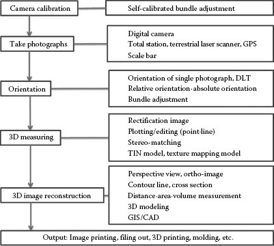
FIGURE 22.2 Process flow.
In the automatic measurement of a surface, it is possible to obtain in short time the 3D data as many as several thousands to several hundred thousands by simply determining the area [4]. And out of these data, we can make polygon and the texture-mapping image pasted with the real picture, which enables us to view the reconstructed image from all angles. All these 3D data can be stored in the files of DXF, CSV, STL, OBJ, and VRML, and used for other purposes, such as creating plan drawing, rapid prototyping, and 3D printing. And if we feed 3D data to point-clouds-based alignment software by the iterative closet point algorithm [15], we can compare the original design data (3D CAD data) with the data obtained by the last measurement and also compare the previous state and the state after the change.
In each following paragraph, each processing is explained according to the process flow of Figure 22.2.
We can make 3D measurement accurate by obtaining interior orientation parameters through camera calibration [2,3]. In this process, with the camera to be calibrated from different angles and directions, we take plural number of pictures on the control points allocated with precision in 3D (Figure 22.3a). And from each of the plural images thus obtained, we extract, by image processing, the control points, and from their coordinates, we calculate their parameters. For simpler way, however, we can use merely a sheet on which control points are printed (Figure 22.3b). For calculation, we use self-calibrated bundle adjustment method in which calibration program is included [5].
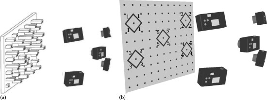
FIGURE 22.3 Camera calibration: (a) 3D field and (b) sheet.
The self-calibrated bundle adjustment is the adjustment that is done by interior orientation parameters that are obtained by integrating correction terms of camera (Equation 22.2: Δx, Δy) simultaneously.
There are different kinds of rectifying model for lens distortion, but common type works in the direction of radiation and tangential line. These equations are as follows [32]:
where
X, Y are image coordinates
Xp, Yp are coordinates of principal point
K1, K2, K3 are radial lens distortion parameters
P1, P2 are tangential lens distortion parameters
r is the distance from principal point to image coordinates
By camera calibration, we can come to the precision as close as 1/1,000–1/20,000 (with a photo distance of 10 m and the difference of less than 0.5 mm) in stereo photogrammetry [6]. There is a report that in the area of industrial measurement (not stereo photogrammetry), where they pasted retro-targets on an object, the accuracy as close as to 1/200,000 was attained [7].
If every camera has already been calibrated, we can make any combination of cameras depending on a project. And if we make shuttering all at the same moment, we can even measure a moving body. And if a scale bar (determined distance between two points) is photographed with an object or if the 3D coordinates of more than three control points are photographed, we can obtain the actual size of the object. Even if there is no control point, we can still make a relative model.
In case of indoor measurement, we take pictures of an object with scale bars (Figure 22.4a). In case of outdoor measurement, we also use surveying instruments such as total station or GPS. If we can place reflective targets (Figure 22.4b) or refractive coded targets (Figure 22.4c) on or around the object, we can introduce automatization, increase accuracy and reliability, and save a lot of time. And the targets would also work as tie points to connect images when we measure a large object or extensive area. It also would serve measuring points of 3D coordinates.
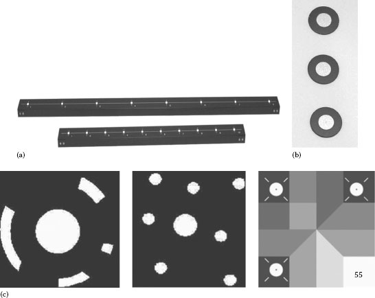
FIGURE 22.4 (a) Scale bar, (b) reflective targets, and (c) reflective coded targets (left: centripetal type, middle: dispersing type, and right: color type).
We can also make a 3D model, detecting the feature points of the image without using targets. But if we have to make the measurement with actual scale with the utmost accuracy, it is necessary to input the distance between feature points or to place the targets as control (measured) points.
With stereo photogrammetry, we can make full automatic stereo-matching of the entire object surface. In this case, however, we need some features on the surface in order to identify the corresponding positions on the right and left images. Ordinarily, if we work with an outdoor object, we have enough features, but if it is a man-made object, oftentimes we do not. In such case, we put features or patterns on the object by a projector or put some paint on its surface. An ordinary projector is good enough.
Exterior orientation is a process to determine the 3D position of the camera and the inclination of three axes (exterior orientation parameters) at the time of measuring. The stereo photogrammetry is possible if we have at least six corresponding points from both pictures for identification. We can make automatic measurement by detecting the feature points through image processing without placing the targets. However, we cannot only simplify but also automatize the process of identification and make the 3D measurement much more accurate by placing specific targets on or around the object. If we can fix the position of cameras and if we determine the exterior orientation parameters beforehand, the identification of the features is not necessary. Furthermore, once we have integrated the bundle adjustment in orientation, we can make image connections on extensive areas, or even all-around modeling, if the data of a scale or 3D coordinates or model (relative) coordinates space are fed to PC.
There are three types of orientation: manual, semiautomatic, and full automatic. For full automatic, however, we need reflective targets or special targets called coded target (Figure 22.4b and c). On these target images, we make target identification automatically. We can also automatically detect the feature points of the image and make identification process without targets. Based on the data of these identified corresponding points (targets), we make exterior orientation and acquire its parameters and 3D coordinates of targets. Even interior orientation parameters can be obtained by this process.
There are three kinds of coded targets (Figure 22.4c): centripetal type (left) [8], dot-dispersing type (middle) [9,10], and color type (right) [11]. We have developed color-coded target, which enabled us to obtain even texture picture and to measure on the surface [11]. As shown in Figure 22.4c (right), the color-coded target consists of a reflective retro-target in three corners and the color section where the position and combination of colors constitute the code. We have 720 combinations as code.
In the stereo photogrammetry, we can relocate the images in such a way that the corresponding points can line up on the epi-polar line (rectified image: Figure 22.1c). Therefore, the searching work of corresponding points can be done only on one line. And if we integrate stereo-matching function here so that the corresponding points on the right and left images can be automatically obtained, we can easily make 3D measurement by semiautomatic operation. The automatic measurement of a surface is the process, which automatically identifies the corresponding points on the right and left images, calculates the data of height, and visualizes or creates the 3D undulation on the surface. We call this digital surface model. For this, we use “area-based” stereo-matching. For this operation, we use not only coarse-to-fine cross-correlation method, but also least squares matching (LSM [4,14]) method to minimize mismatching on the project distortion or tilted parts. Presently, standard deviation of LSM is reported as 0.26 mm and that of normalized-cross-correlation method is 0.35 mm. There is also report that LSM is more accurate in inclined object than normalized-cross-correlation method [6,35].
In the research of industrial measurement, there is a report of 0.077–0.205 mm [23,33,34]. In addition, combining feature-based matching and area-based matching, we have also developed the stereo-matching method, which is robust to brightness change and occlusion [35,36].
22.2.2.5 3D Image Reconstruction and Output
To make 3D model, we work with the triangle irregular network (TIN) model by using Delaunay triangulation [37], considering the measuring points not as the group of points but as a surface. TIN model (Figure 22.5) can reconstruct the smooth surface, if mismatching is eliminated.
In our method, as the correlation between the photographed image and the 3D position of the points measured from each stereo model is already established, it is not necessary to match texture with TIN model. As to the texture image, we can make the texture mapping with the same degree of resolution as at the time of measuring, if the image is the image used for measuring, because the texture image makes simultaneously the adjustment of camera lens distortion and project distortion at the time of photographing. And the 3D model with texture can be turned around or enlarged or downsized as we wish and can be studied from all sides on the PC display. If we output the measured result as ortho-photo with texture, it would reflect the actual size. And if we output as DXF, VRML, OBJ, or STL file and feed the molding system, we can make replica made by 3D printer as well as compare with CAD.
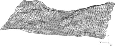
FIGURE 22.5 Triangle irregular network (TIN).
22.2.3 PHOTOGRAMMETRIC SLAM (VISUAL SLAM, SFM)
Computer vision is the method to process the enormous amount of still images and video image. They are the methods called structure from motion (SFM [38,39,40]) or visual simultaneous localization and mapping (SLAM). They are the methods to reconstruct 3D images, simultaneously estimating camera’s position and inclination out of the scenes taken by photographs.
The analytic calculation differs in the photogrammetry and the computer vision. But the basic principle is the same as the ones explained in Section 22.2.1. And the method by photogrammetry is called photogrammetric SLAM.
Basic principle (see Figure 22.6)
1. We obtain the feature points detected from the two images. And we calculate the 3D of the corresponding points from the forward intersection. For the matching of the feature points, we use feature-based matching, such as SIFT [41] and SURF [42].
2. We remove mismatchings.
3. We calculate the exterior orientation from 3D coordinates (space resection).
4. We repeat this process in the orderly way.
We make the bundle adjustment during and at the end of the process to minimize the errors. Various studies are made to improve the integration of the bundle adjustment [27,43,44,45,46,47].
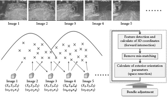
FIGURE 22.6 Photogrammetric SLAM.
22.3 APPLICATION EXAMPLES OF 3D MEASUREMENT AND MODELING
We are striving to develop the technology of measuring various objects in 3D using our software of digital photogrammetry. The explanations of the examples are given in the following sections.
22.3.1 APPLICATION OF CULTURAL HERITAGE, ARCHITECTURE, AND TOPOGRAPHY
22.3.1.1 3D Modeling of Wall Relief
We made 3D modeling of a wall relief at the Acropolis Theatre of Dionysus in Greece [13]. We used an ordinary digital camera (5 million pixels). We took two pictures of the relief. On the relief pictures of left and right, we simply marked 10 corresponding points on each pictures for orientation as in Figure 22.7a and made automatic measuring. As the automatic measurement takes only a few minutes, the modeling of the whole picture was finished in less than 10 min. Figure 22.7b is the image obtained by rendering from the measured result and by adding contour lines. Figure 22.7c is the bird’s view. We can see from the result how the relief is successfully 3D modeled in great details.
22.3.1.2 Byzantine Ruins on Gemiler Island
The Byzantine ruins on Gemiler Island, which is located off the Lycian coast of southern west of Turkey, has been studied by the research group of Byzantine Lycia, a Japanese joint research project [16]. The Church II we photographed was about 10 m × 10 m. The camera was Kodak DCS Pro-Back (16 million pixels; body, Hasselblad 555ELD; and lens, Distagon 50 mm). We took two stereo images with the shooting distance 16 m, the base length 6 m, and the focal length 52 mm. To obtain the actual measurement, we used the survey instrument total station to determine three points as the reference points. Under these conditions, the pixel resolution was 3 mm for horizontal direction and 8 mm for depth direction. A triangulated irregular network (TIN) model has been automatically created, and the number of produced points was about 260,000. Figure 22.8a is the photographed image of Church II. Figure 22.8b is the rendering image reconstructed on the PC after measuring, and Figure 22.8c illustrates different view of the same model. Furthermore, to evaluate the accuracy, we compared the ortho-photo image with the elevation plan. We were able to superimpose even the fissures within the range of less than 1 cm [6,35]. As for other examples in this site, we made 3D models and digital ortho-photos of the floor mosaic, which we analyzed and compared with the drawing [17,35].
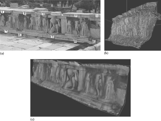
FIGURE 22.7 3D modeling of wall relief: (a) orientation, (b) after rendering and contour lining, and (c) bird’s view.
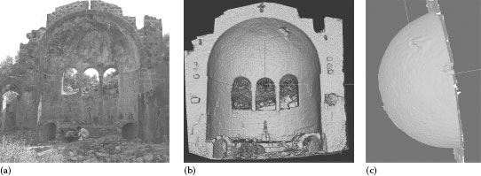
FIGURE 22.8 Byzantine ruins in Gemiler Island: (a) photographed image of Church II, (b) rendering image (front), and (c) different view.
22.3.1.3 All-Around Modeling of a Sculpture in the Archaeological Museum of Messene in Greece
The lion statue was found from Grave Monument K1 in Gymnasium complex buildings and is now kept at the Archaeological Museum of Messene in Greece. The lion is hunting a deer from behind (Figure 22.9a). This lion statue is considered to be on top of the Grave Monument roof. As this sculpture (its front part as in Figure 22.9a) was placed only 1 m away from the back wall, the photographing distance from the back was short. So we had to take many pictures. And as we did not use the light fixture, the brightness of each picture is different. The digital camera we used had 6 million pixels with single lens reflex (SLR) type (Nikon D70), with lens focal length of 18 mm. We took 100 pictures from all around, of which 20 were used for modeling.
The result of the all-around modeling is shown in Figure 22.9b and c. The reason why the color of texture mapping is different is due to the difference in brightness at the places of shooting.
As for other examples of the pictures taken for measuring in this archeological site of ancient city Messene, we have that of an architectural member of a relief, which we analyzed and compared with the drawing [18].
22.3.1.4 All-Around Modeling of the Church of Agia Samarina
The Byzantine church of Agia Samarina is located 5 km south of Ancient Messene (Figure 22.10a). This church was renovated from ancient building (probably a kind of temple) to Byzantium church, so big limestone blocks were used in the lower part of the church. We used the same digital SLR camera with 18 mm wide angle lens. The environment of taking photo was as follows: object distance was about 11 m, distance between viewpoints was about 4 m, and 34 photos were used to make the 3D model. In this situation, 1 pixel was about 4.5 mm in horizontal direction and about 15 mm in vertical direction. Figure 22.10b shows the 3D wire flame model with texture mapping, and Figure 22.10c shows the digital ortho-photo of the 3D model. While we could not get the pictures of higher parts like roof, as taken from the ground, as you see in these pictures, we succeed in making digital ortho-photos of the elevation of this church.
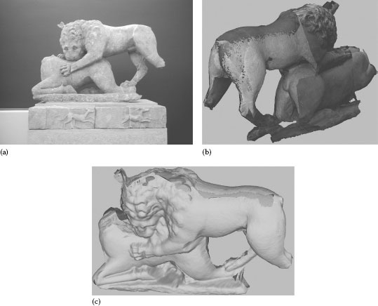
FIGURE 22.9 (a) Lion devouring a deer, (b) texture mapping, and (c) rendering.
We took two pictures of topography from a helicopter with a digital camera [19]. Then, we made 3D measurement from the pictures and produced a diorama out of the data. We used a digital camera of SLR type with 6 million pixels and with 20 mm wide angle lens.
As the control points, we used six points measured by GPS. The helicopter altitude was 230 m, and the distance between cameras was 53.4 cm with the resolution capacity 9 cm horizontally and 38 cm in depth. Figure 22.11a shows the picture taken. Figure 22.11b and c shows the picture of the diorama produced by rapid prototyping from the modeling data, with thermoplastics (Figure 22.11b) and paper (Figure 22.11c) as base material.
22.3.1.6 3D Model Production with Aerial and Ground Photographs
We produced 3D model by putting together the data from aerial pictures, the pictures taken from a paraglider, and the pictures taken on the ground by digital cameras. The object is the Topcon main building in Itabashi ward of Tokyo, Japan [20].
The pictures we used were the aerial photo by the film camera of airplane, the photo by digital camera of powered paraglider, and the lateral photo obtained by digital camera on the ground. The area of the each photo we used for modeling was about 300 m × 300 m, 100 m × 50 m, and 20 m × 20 m.
We first produced 3D model for each of them by our software (PI-3000, Image Master) and then fused them together. As for the control points, we first measured the side of the building by reflectorless total station [21,61] and converted the data to GPS coordinate using the points measured by GPS in the building lot.
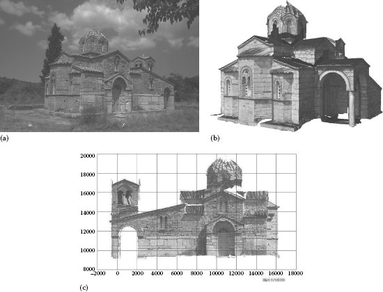
FIGURE 22.10 (a) Byzantium church of Agia Samarina, (b) 3D model, and (c) digital ortho-photo image.
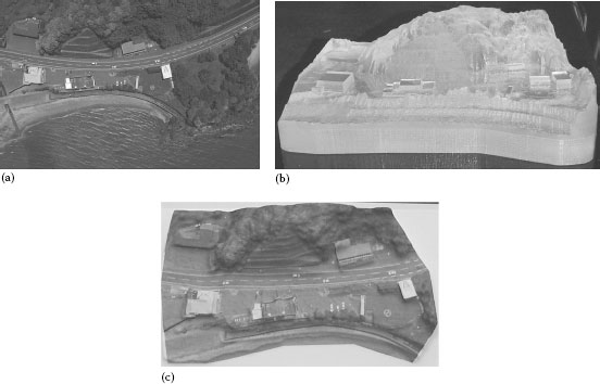
FIGURE 22.11 Topography model: (a) picture taken, (b) diorama (thermoplastics), and (c) diorama (paper).
TABLE 22.1
Cameras Used for High-, Low-, and Ground-Level Photographs and Conditions
Camera |
Airplane |
Paraglider |
Ground |
WILD RC-20 |
CANON EOS Digital |
Minolta Dimage7 |
|
Sensor |
Film |
C-MOS (22.7 mm × 15.1 mm) |
CCD (2/3 in.) |
Number of pixels |
6062 × 5669 (by Scanner) |
3072 × 2048 |
2568 × 1928 |
Resolution |
42.3 μm |
7.4 μm |
3.4 μm |
Focal length |
152.4 mm |
18 mm |
7.4 mm |
Photographing Area |
2000 m × 2000 m |
200 m × 100 m |
30 m × 25 m |
Modeling area |
300 m × 300 m |
100 m × 50 m |
20 m × 20 m |
Altitude |
1609 m |
163 m |
26(side)m |
Base length |
886 m |
18 m |
5 m |
Resolution: ΔXY |
0.89 m |
0.06.6 m |
0.01 m |
Resolution: ΔZ |
1.61 m |
0.6 m |
0.06 m |
Table 22.1 shows the capacity of the cameras used for high-, low-, and ground-level photographs and the conditions for analysis by each camera. And Figure 22.12a is the display of PI-3000 (Image Master) showing all of the analysis of each camera. Figure 22.12b shows the digital photograph by powered paraglider, and Figure 22.12c and d shows the results of the 3D model with texture mapping.
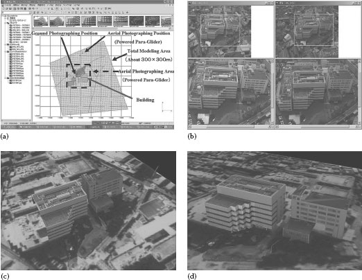
FIGURE 22.12 (a) All of the analysis of each camera, (b) digital photograph by powered paraglider, and (c, d) different views of the 3D model with texture mapping.
22.3.2 APPLICATION TO HUMAN BODY MEASUREMENT
The digital photogrammetry has an advantage to obtain the picture of the exact state of a moving object at a certain given moment [22]. To give an example, we worked on measuring human face and body.
We made 3D modeling of a human face and used it for 3D simulation of ophthalmology equipment designing. Since there are people whose faces have less features than others, we took pictures with random-dot patterns projected by an ordinary projector. We also took pictures without dots for texture mapping. We used two digital SLR cameras of 6 million pixels with 50 mm lens in stereosetting. Photographing conditions were as follows: distance was 1 m, distance between cameras was 30 cm, and resolution capacity was 0.2 mm horizontally and 0.5 mm in depth.
Figure 22.13 shows the result of photo measuring. Figure 22.13a is the texture-mapped picture without patterns. Figure 22.13b is the result of measuring the cross section. The 3D data obtained by modeling was fed to 3D CAD, and the image of 3D CAD was created, simulating a person putting chin on the ophthalmology equipment (Figure 22.13c). This enables us to determine the optional relation between the equipment and the face in 3D, the data necessary to make the design of the equipment.
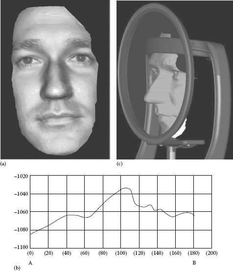
FIGURE 22.13 3D modeling of human face: (a) texture mapping, (b) cross section, and (c) simulation with 3D CAD.
We set up four stereo-cameras facing each other at an angle of 90° around the body. This enables us to make all-around measurement without being disturbed by the body movement. Here, we made all-around images on the human body of a female. As shown in Figure 22.14a, we set up a projector behind each stereo-camera. For this photographing, we made two kinds of images: those with projected random patterns and those without them. All four stereo-cameras were identical in structure and in applied conditions. They were all SLR-type digital camera of 6 million pixels with the lens of 28 mm focal length. The photographing conditions were as follows: photographing distance was 1.3 m, distance between cameras was 0.3 m, resolution was horizontally 0.28 mm and in depth 1.3 mm. Figure 22.14b and c shows the measurement results of surface model and texture-mapping model. Thus equipped with easily obtainable cameras and projectors, we were able to measure human body and with considerable precision [36].
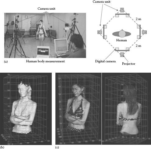
FIGURE 22.14 Human body measurement: (a) photographing setup, (b) result of surface model, and (c) result of texture-mapping model.
22.3.3 APPLICATION TO AUTOMOBILE MEASUREMENT
There are many different things to be measured in automobile, for example, small parts to middlesized parts like seat, as well as large parts like bottom or entire body. So, we have measured them with digital cameras and our software and proved its feasibility [23], as explained in the following sections.
In auto accident, it is often extremely difficult and complicated to precisely measure and record the deformation and debris and to visualize it in image. Therefore, we photographed and measured the bottom of a car and visualized it. Figure 22.15a shows the bottom width 1.5 m × length 4.5 m. We used one digital SLR camera of 6 million pixels. We used lens of focal length 20 mm.
We lifted a car by crane, placed camera in 18 positions (in 3 lines with 6 positions in each) (Figure 22.15b), and shot upward (Figure 22.15c). The bottom part has lots of dirt, which served as a texture. So, pattern projection was not necessary. Photographing distance was about 1.7 m, and the distance between cameras was 0.5 m. As to the precision, the standard deviation was 0.6 mm in plane and 2 mm in depth. It took 1 h to photograph, and the analysis of 16 models (32 pictures) took almost a day. The results are shown in Figure 22.16.
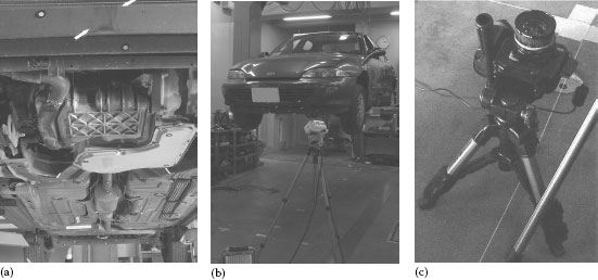
FIGURE 22.15 Car measurement: (a) bottom, (b) photo position, and (c) photographing.
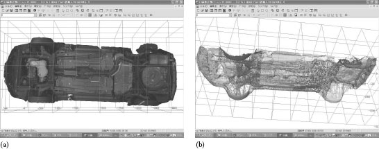
FIGURE 22.16 Car measurement result: (a) texture mapping and (b) wire frame.
22.3.3.2 Measuring Surface of the Entire Body
Measuring an entire body is necessary, for example, in auto accident site or industrial production of a clay model. We made all-around measurement of a car by two different ways: with solely point measurement and with surface measurement.
1. Automatic point measurement of a vehicle by coded targets: it is reported that in order to simplify the measuring of a damaged car, coded targets had been pasted on its surface for automatic measurement [24]. Therefore, we placed color-coded targets on a car and made all-round automatic measurement. The number of images or photos was 36, of which stereo-pairs were 32. Figure 22.17a is the result of the target identification detected automatically. You can see three retro-targets labeled with a number.
As to the accuracy, the error of transformation in the color-code recognition or the error of wrong recognition of target in the place where it does not exist was none. The rate of false detection was zero. Figure 22.17b shows the 3D measuring result of detected points.
2. All-around measurement of a car body by stereo-matching: as shown in Figure 22.18a, we used a stereo-camera and a projector. We photographed from eight different positions around the car, each from both upper angle and lower angle (16 models altogether). We also photographed the roof from above and this in four positions on the left and four positions on the right. All these totaled to 32 models with 64 images altogether. Furthermore, for each of these 64, we took pictures with patterns and without patterns. This means we photographed 128 images altogether for analysis (Figure 22.18b). We used digital cameras Nikon D70 of 6 million pixels and attached a lens of focal length 28 mm. For each model, the photo distance was about 2 m. The distance between cameras was 0.95 m. Given this photographing condition, the measuring area of one model is 1 m × 0.7 m, and the measuring accuracy is about 0.5 mm in plane and 1.2 mm in depth. Including the time to attach the targets, it took about 2 h to photograph and 1.5 days to analyze. Figure 22.19 shows the resulted texture mapping, wire frame, and mesh form. Here, the window is shown simply as a plane, since we could not measure the window glasses. The transparent parts like lights and black parts like door knobs cannot be measured. If we want to measure them, we must paint or put powder on them.
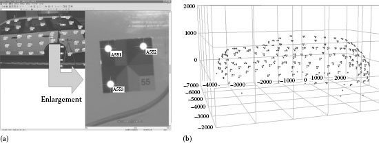
FIGURE 22.17 (a) Result of target identification and (b) 3D measuring result of detected points.
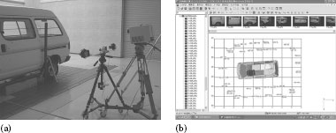
FIGURE 22.18 All-around measurement of a car body by stereo-matching: (a) photographing and (b) photo position.
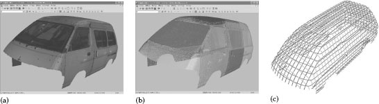
FIGURE 22.19 The measured result of Figure 22.18: (a) texture mapping, (b) wire frame, and (c) mesh form.
22.3.3.3 Measuring Surface of the Tire
This is to show the new measuring method we have developed.
Area-based matching methods set an image area as a template and search the corresponding match. As a direct consequence of this approach, it becomes not possible to correctly reconstruct the shape around steep edges. Moreover, in the same regions, discontinuities and discrepancies of the shape between the left and right stereo-images increase the difficulties for the matching process. In order to overcome these problems, we have developed the approach of reconstructing the shape of objects by embedding reliable edge line segments into the area-based matching process. We have developed a robust stereo-matching method that integrates edges and which is able to cope with differences in right and left image shapes, brightness changes, and occlusions [49,50].
The method consists of the following three steps: (1) parallax estimation, (2) edge-matching, (3) edge-surface matching.
Here, as an example, we measured a tire, using its algorithm.
We tried to find whether it is possible to show clearly the structural feature of a tire with deep groove. We obtained 144,991 points separated from each other by 1 mm. Figure 22.20a is the original picture. Figure 22.20b shows the result of overlapping the stereo-matching result onto the detected edge image. On the surface of tire, we can see the color-coded targets for orientation and the groove. Figure 22.20c shows the matching result without edge-matching. Figure 22.20d shows the result of the edge-surface matching by detecting 3D edge in our new method. Figure 22.20e shows the line profile of each method. Here we can see clearly the feature of the groove, which cannot be obtained without edge-matching.
We made an accuracy assessment, using the tire (Figure 22.21a), which we measured with the contact 3D measuring device (Zeiss UMC550S: accuracy 10 μm). We compared the cross section of our new method and the contact 3D measuring device. We mounted 35 mm lens to the Nikon SLR camera and took stereo picture with the photographing distance 618 mm and base length 240 mm. The resolution for this work was Δxy: 0.1 mm for plane and Δz: 0.26 mm for depth. Table 22.2 shows the result. Figure 22.21b shows the cross section of the comparison between contact 3D measuring device and edge-surface matching. For line 1, the average was 0.09 mm, standard deviation was 0.1 mm, and maximum difference was 0.4 mm. For line 2, the average was 0.14 mm, standard deviation was 0.14 mm, and maximum was 0.5 mm.
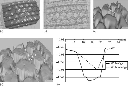
FIGURE 22.20 (a) Original image, (b) edge detection + stereo-matching, (c) result of surface matching (without edge), (d) result of edge-surface matching, and (e) result of measurement compared with surface matching.
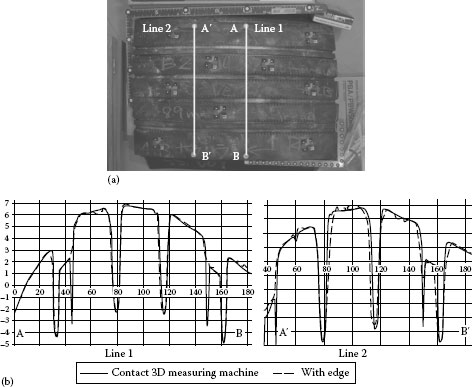
FIGURE 22.21 (a) Evaluation line and (b) comparison between contact 3D measuring device and edge-surface matching.
Table 22.2 Accuracy Assessment
Line 1 |
Line 2 |
|
Number of points |
51 |
49 |
Average |
0.09 mm |
0.14 mm |
Standard deviation |
0.10 mm |
0.14 mm |
Maximum |
0.4 mm |
0.5 mm |
While in the usual method, the groove measuring gauge of tire is ±0.1 mm for point measurement, in the new method, we can measure even the surface as the evaluation of tire wear.
This paragraph shows the application of indoor measurement.
Indoor measurement is difficult, as the features are poor and 3D model creation is not easy. Therefore, the effort to develop the model is made, using the edge information and plane information.
For example, the method is recommended that uses the Manhattan world hypothesis [51]. This hypothesis considers basically that the building is composed of three vectors perpendicular to each other. This method is to roughly reconstruct the indoor structure out of many images and often used for walk-through [52].
We propose an automated technique for creating a simplified 3D structure shape model of indoor environments from the sparse 3D point information provided by the photogrammetric method [53].
Figure 22.22 shows the overview of the proposed system.
1. Multiple coded targets (see Figure 22.4c, right) are used for the automatic detection, recognition, and measurement of 3D coordinates of points on the room walls from the acquired stereo images.
2. The sparse 3D information is then processed.
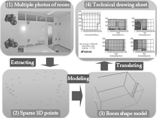
FIGURE 22.22 Overview of the proposed system. (1) Color-coded targets are placed on the walls of a room and stereo images are processed photogrammetrically, (2) sparse 3D points coordinates are obtained. (3) A simplified 3D structure shape model of the room is constructed from the sparse 3D information. (4) The development figure is generated by orthographic projection of the 3D model.
3. A simplified 3D structure shape model of the room is estimated.
4. Additionally, the 3D model is also translated into a development figure that represents multiple orthographic projections of the room.
This method is implemented into a flawless procedure that allows to obtain, by a few operations, a simplified 3D structure shape model of a room and its orthographic representation in drawing sheets. The developed application software can be used for the determination of the shape of rooms easily also by persons without experience in 3D measurement techniques.
The basic principle of measuring that uses SFM and SLAM in the computer vision was explained in Section 22.2.3. The well-known system that uses the image sequence is PTAM [54], and the one that uses the still image is photo tourism [55]. PTAM makes augmented reality (AR) of small space from a video-camera. Photo tourism is a web system to enjoy the virtual tourism, using the 3D reconstruction out of tourism pictures.
The followings are what we are trying to do as photogrammetric SLAM.
22.3.5.1 Measurement by Vehicle (Measurement by Image Sequences)
Here is an example of measuring big pile of earth by putting a video-camera on top of the car [56]. Figure 22.23a shows the camera and GPS on the car. Figure 22.23b shows the actual operation of measurement.
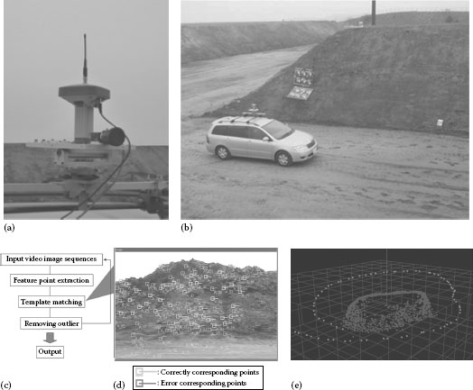
FIGURE 22.23 Measurement by vehicle: (a) camera and GPS on the car, (b) measuring, (c) flow of image tracking, (d) tracking feature points, and (e) result.
We obtain the feature points by tracking the image sequences from the video-camera, and from the feature points, we obtain the camera’s position and the 3D coordinates of the object. Figure 22.23c and d shows the flowchart of image tracking and feature points tracking. The process of image tracking is as follows:
1. Input of video image
2. Detecting the feature points by image processing
3. Matching of adjacent pictures of the feature points detected
4. Removing the errors
We repeat (1)–(4) processes orderly.
We simultaneously seek camera’s position and the 3D coordinates of the object from the feature points detected, calculating the exterior orientation parameters and the 3D coordinates in order. Figure 22.23e shows the result. You can see the trajectory of the car and the big pile of the earth (in our example, we did not use GPS).
In the ordinary mobile mapping system, we obtain the 3D model by laser scanner and obtain the car position by using GPS, IMU, and odometer. And we combine these images with measuring instruments.
22.3.5.2 Measurement by UAV (Measurement by Image Sequences and Still Images)
The low-cost unmanned aerial vehicle (UAV) has become useful tool for low-altitude photogrammetry from the rapidly increasing automatic control technique in the past several years. Figure 22.24a shows an example of UAV.
In this paragraph, we show the automatic exterior orientation procedure and reconstruct the 3D model for the low-cost UAV photogrammetry. We have developed the automatic corresponding point detection technique using both video image and still images [57]. The video image is obtained with still images simultaneously. Therefore, the tracking result of video image gives robust correspondence information between each of the still images. Moreover, the exterior orientation procedure using GPS information from UAV and minimum ground control points has been investigated. For model making, we used the method of area-based matching, which can show the edges clearly in details.
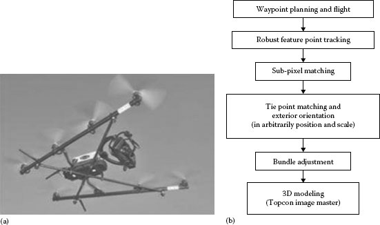
FIGURE 22.24 (a) UAV and (b) flow of automatic measurement.
The following are the flow of the measurement (Figure 22.24b):
1. The waypoint planning and flight control are performed. High-resolution still images at waypoints, video image during flight, and also positioning information of each waypoint are obtained as a result of a flight.
2. At the beginning of this process, the detection of common feature points from high-resolution still image and tracking of detected feature points on video image sequences are performed using robust feature point tracking method [57]. The tracking result of feature points are obtained in the image coordinate on high-resolution still image.
3. Then, sub-pixel matching of each feature point is performed. The good results of this subpixel matching are used as candidate of correct pass points.
4. In order to perform tie-point matching, the exterior orientation using these candidate pass points is performed. The result of exterior orientation in this step gives the geometry of candidate pass points and still images in arbitrarily position and scale.
5. Next, registration in global coordinate using the positioning information of waypoints and minimum ground control points is performed by using bundle adjustment with robust regression.
6. Finally, we make 3D model reconstruction by edge-surface matching (Section 22.3.3.3), which we have developed [49,50].
We took pictures of the area (50 m × 50 m) from 30 m high using UAV.
Figure 22.25a shows the result of the stereo-matching, using 157 images with the additional texture mapping (without using edge-surface matching). Figure 22.25b through d shows the result of the edge-surface matching. Figure 22.25c is the result of texture mapping, Figure 22.25d is the result of 3D edge detection. As you can see, without using edge-surface matching method (Figure 22.25a), the features are not so clear, while, as shown in Figure 22.25b and c, the features are clear.
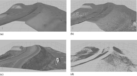
FIGURE 22.25 Measurement result (a) without edge-surface matching, (b) edge-surface matching, (c) texture mapping with edge-surface matching, and (d) 3D edge.
Figure 22.26 shows the result of measuring the staircase with 25 pictures from 15 m high. We can clearly see the features (Figure 22.26b and c), which could not be shown clearly by the method without using edge-surface matching (Figure 22.26a).
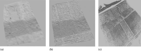
FIGURE 22.26 Measurement result of staircase (a) without edge-surface matching, (b) edge-surface matching, and (c) 3D edge.
As digital photogrammetry can make 3D measuring and modeling out of plural number of pictures obtained by digital camera, it has an array of advantages as follows:
1. As the equipment requirement is as simple as a digital camera and a PC, we can easily take it out to any place. We can also use as many kinds and numbers of cameras as we wish.
2. Basically, there is no limit to the kind and size of an object from minimum to maximum. It can even measure an object from all around.
3. Utilization for moving object: 3D measuring and modeling of movable object is possible in its state of given instance, including such object as human body.
4. We can use it for a wide variety of purposes, such as plan drawing and model making that require 3D data. It can be also used for reverse engineering and such works as comparing and inspecting with CAD data.
5. Utilization of texture: as we obtain 3D data from pictures, we cannot only grasp the object visually but also make 3D measurement through image processing and produce orthoimage as well.
And from its wide range of possible applications and developments, there are other important spillouts such as the ones shown as follows:
1. Utilization of moving image: 3D measurement and modeling using a video-camera [25,26,27,46,47,54].
2. Utilization for the image of electro-microscope: 3D measurement from the scanning electron microscope image [28].
3. Application for image recognition: utilization of 3D data for facial image recognition [29].
4. Utilization for multi-oculus 3D display system: we can use this for the data display of multi-oculus 3D display system (e.g., 128 eyes), which makes it possible for many people to see together the 3D reality without stereo-glasses [30].
5. Utilization for sensor fusion technology: it is a 3D measurement technology to integrate and use the data obtained through cameras and various sensors (GPS, total station, position sensor, laser scanner, etc.) put on a robot or car [1,31].
6. Model synthesizing and automatization of whole process: synthesizing the point cloud obtained by laser scanner and the 3D point cloud obtained from the images. The researches first used the laser scanner to take the dense point cloud of small areas and the photogrammetry of UAV to take the large area [58,59]. And then contrariwise, we took the picture of the large areas by the laser scanner, and the small areas by photogrammetry of handy digital camera [49]. And we synthesize them together. Thus, we achieved the total automatization and speeding up of model production and mapping.
7. Integration of 2D image and 3D point cloud, and processing and recognition: the technology of the registration and the object recognition, using the image features and shape features, is an important goal we are presently challenging [48,49,60].
Though we could not present other examples in these limited pages, we believe that the future of digital photogrammetry is almost unlimited as the presented examples indicate.
1. Urmson, C., Wining the DARPA urban challenge—The team, the technology, the future, Fifth Annual Conference on 3D Laser Scanning, Mobile Survey, Lidar, Dimensional Control, Asset Management, BIM/CAD/GIS Integration, SPAR2008, Spar Point Research, Houston, TX, 2008.
2. Kochi, N. et al., 3 Dimensional measurement modeling system with digital camera on PC and its application examples, International Conference on Advanced Optical Diagnostics in Fluids, Solids and Combustion, Visual Society of Japan, SPIE, Tokyo, Japan, 2004, p. V0038-1-10.
3. Kochi, N. et al., PC-based 3D image measuring station with digital camera an example of its actual application on a historical ruin, ISPRS, Ancona, Italy, 34, 195–199, 5/W12, 2003.
4. Kochi, N. et al., 3D-measuring-modeling-system based on digital camera and pc to be applied to the wide area of industrial measurement, The International Society for Optical Engineering (SPIE) Conference on Optical Diagnostics, San Diego, CA, 2005.
5. TOPCON CORPORATION, Products and applications, 2009–2014, http://www.topconpositioning.com/products/ (accessed November 27, 2014).
6. Karara, H. M., Introduction to metrology concepts, Analytic data-reduction schemes in non-topographic photogrammetry, Camera calibration in non-topographic photogrammetry, Non-Topographic Photogrammetry, 2nd edn., McGlone, J. C. (ed.), American Society for Photogrammetry and Remote Sensing, Falls Church, VA, Chapters 2, 4, 5, 1989.
7. Slama, C. C., Basic mathematics of photogrammetry, Non-Topographic photogrammetry, Manual of Photogrammetry, 4th edn., Karara, H. M. (ed.), American Society for Photogrammetry and Remote Sensing, Falls Church, VA, Chapters 2, 16, 1980.
8. Schenk, T., Digital Photogrammetry, Vol. 1, Terra Science, Laurelville, OH, 1999.
9. Heipke, C., State-of-the-art of digital photogrammetric workstations for topographic applications, Photogrammetric Engineering and Remote Sensing, 61(1), 49–56, 1995.
10. Noma, T. et al., New system of digital camera calibration, ISPRS Commission V Symposium, Corfu, Greece, 54–59, 2002.
11. Brown, D. C., Close-range camera calibration, Photogrammetric Engineering, 37(8), 855–866, 1971.
12. Fraser, C. S., Shotis, M. R., and Ganci, G., Multi-sensor system self-calibration, Videometrics IV, 2598, 2–18, SPIE, 1995.
13. Heuvel, F. A., Kroon, R. J. G., and Poole, R. S., Digital close-range photogrammetry using artificial targets, ISPRS, Washington, DC, 29(B5), 222–229, 1992.
14. Hattori, S. et al., Design of coded targets and automated measurement procedures in industrial visionmetrology, ISPRS, Amsterdam, the Netherlands, 33, WG V/1, 2000.
15. Ganci, G. and Handley, H., Automation in videogrammetry, ISPRS, Hakodate, Japan, 32(5), 47–52, 1998.
16. Moriyama, T. et al., Automatic target-identification with color-coded-targets, ISPRS, Beijing, China, 21, WG V/1, 2008.
17. Kochi, N., Ito, T., Kitamura, K., and Kaneko, S., Development of 3D image measurement system and stereo-matching method, and its archaeological measurement, Electronics and Communications in Japan, 96(6), 9–21, 2013.
18. Grun, A., Adaptive least-squares correlation: A powerful image matching technique, South Africa Journal of Photogrammetry, Remote Sensing and Cartography, 14(3), 175–187, 1985.
19. Besl, P. J. and McKay, N. D., A method for registration of 3D shapes, IEEE Transaction on Pattern Analysis and Machine Intelligence, 14(2), 239–256, 1992.
20. Bethmann, F. and Luhmann, T., Least-squares matching with advanced geometric transformation models, ISPRS, Vol. XXXVIII, Part 5 Commission V Symposium, Newcastle upon Tyne, U.K., 2010, pp. 86–91.
21. Luhmann, T., Bethmann, F., Herd, B., and Ohm, J., Experiences with 3D reference bodies for quality assessment of freeform surface measurements, ISPRS, Vol. XXXVIII, Part 5 Commission V Symposium, Newcastle upon Tyne, U.K., 2010, pp. 405–410.
22. Kitamura, K., Kochi, N., Watanabe, H., Yamada, M., and Kaneko, S., Human body measurement by robust stereo matching, Ninth Conference on Optical 3-D Measurement Techniques, Vol. 2, 2009, pp. 254–263.
23. Aurenhammer, F., A survey of a fundamental geometric data structure, ACM Computing Surveys, 23(3), 345–405, 1991.
24. Beardsley, P., Zisserman, A., and Murray, D., Sequential updating of projective and affine structure from motion, International Journal of Computer Vision, 23(3), 235–259, 1997.
25. Tomasi, C. and Kanade, T., Shape and motion from image streams under orthography: A factorization method, International Journal of Computer Vision, 9(2), 137–154, 1992.
26. Pollefeys, M., Koch, R., Vergauwen, M., Deknuydt, A., and Gool, L.J.V., Three-dimensional scene reconstruction from images, Proceedings of the SPIE, 3958, 215–226, 2000.
27. Lowe, D., Distinctive image features from scale invariant keypoints, International Journal of Computer Vision, 60(2), 91–110, 2004.
28. Bay, H., Ess, A., Tuytelaars, T., and Gool, L., Speeded-up robust features (SURF), Computer Vision and Image Understanding, 110, 346–359, 2008.
29. Anai, T., Kochi, N., and Otani, H., Exterior orientation method for video image sequences using robust bundle adjustment, Eighth Conference on Optical 3-D Measurement Techniques, Vol. 1, Zurich, Switzerland, 2007, pp. 141–148.
30. Mouragnon, E., Lhuillier, M., Dhome, M., Dekeyser, F., and Sayd, P., Real time localization and 3D reconstruction, Proceedings of the 2006 IEEE Computer Society Conference on Computer Vision and Pattern Recognition, Vol. 1, New York, NY, 363–370, 2006, pp. 363–370.
31. Eudes, A. and Lhuillier, M., Error propagations for local bundle adjustment, CVPR’09, Miami, Florida, 2411–2418, 2009.
32. Mouragnon, E., Lhuillier, M., Dhome, M., Dekeyser, F., and Sayd, P., Generic and real time structure from motion using local bundle adjustment, Image and Vision Computing, 27(8), 1178–1193, 2009.
33. Fukaya, N., Anai, T., Sato, H., Kochi, N., Yamada, M., and Otani, H., Application of robust regression for exterior orientation of video images, ISPRS, Beijing, China, XXIth Congress, WG III/V, 2008, pp. 633–638.
34. Anai, T., Fukaya, N., Sato, T., Yokoya, N., and Kochi, N., Exterior orientation method for video image sequences with considering RTK-GPS accuracy, Ninth Conference on Optical 3-D Measurement Techniques, Vol. 1, Viena, Austria, 2009, pp. 231–240.
35. Tsuji, S. et al., The Survey of Early Byzantine Sites in Oludeniz Area (Lycia, Turkey), Osaka University, Osaka, Japan, 1995.
36. Kadobayashi, R. et al., Comparison and evaluation of laser scanning and photogrammetry and their combined use for digital recording of cultural heritage, ISPRS, Istanbul, Turkey, 20th Congress, WG V/4, 2004.
37. Yoshitake, R. and Ito, J., The use of 3D reconstruction for architectural study: The Askleption of ancient Messene, 21st International CIPA Symposium, Athens, Greece, 2007, Paper No. 149.
38. Smith, C. J., The mother of invention—Assembling a low-cost aerial survey system in the Alaska wilderness, GEOconnexion International Magazine, 26–29, December 2007, 20–22, February 2008.
39. Otani, H. et al., 3D model measuring system, ISPRS, Istanbul, Turkey, 20th Congress, WG V/2, 2004, pp. 165–170.
40. Ohishi, M. et al., High resolution rangefinder with a pulsed laser developed by an under-sampling method, SPIE Optical Engineering, 49(6), 064302-1-8, 2010.
41. D’Apuzzo, N., Modeling human face with multi-image photogrammetry, Three-Dimensional Image Capture and Applications V, Corner, B. D., Pargas, R., Nurre, J. H. (eds.), Proceedings of SPIE, Vol. 4661, San Jose, CA, 2002, pp. 191–197.
42. Fraser, C. S. and Clonk, S., Automated close-range photogrammetry: Accommodation of non-controlled measurement environments, Eighth Conference on Optical 3-D Measurement Techniques, Vol. 1, Zurich, Switzerland, 2007, pp. 49–55.
43. Kochi, N., Kitamura, K., Sasaki, T., and Kaneko, S., 3D modeling of architecture by edge-matching and integrating the point clouds of laser scanner and those of digital camera, XXII Congress of the International Society for Photogrammetry, Remote Sensing, Vol. XXXIX-B5, Melbourne, Victoria, Australia, 2012, V/4, pp. 279–284.
44. Kochi, N., Sasaki, T., Kitamura, K., and Kaneko, S., Robust surface matching by integrating edge segments, ISPRS Annals of the Photogrammetry, Remote Sensing and Spatial Information Sciences, Volume II-5, 203–210, 2014.
45. Vanegas, C. A., Aliaga, D. G., and Benes, B., Building reconstruction using Manhattan-World grammars, 2010 IEEE Conference on Computer Vision and Pattern Recognition (CVPR), San Francisco, CA, June 13–18, 2010, pp. 358–365.
46. Furukawa, Y., Curless, B., and Sieitz, S., Reconstructing building interiors from images, ICCV, Kyoto, Japan, 80–87, 2009.
47. Hirose, S., Simple room shape modeling with sparse 3D point information using photogrammetry and application software, ISPRS—International Archives of the Photogrammetry, Remote Sensing and Spatial Information Sciences, 2012, XXXIX-B5, pp. 267–272.
48. Klein, G. and Murray, D., Parallel tracking and mapping for small AR workspaces, ISMAR07, Nara, Japan, November 2007.
49. Snavely, N., Seitz, S., and Szeliski, R., Photo tourism: Exploring photo collections in 3D, ACM Siggraph, 25(3), 835–846, 2006.
50. Anai, T., Kochi, N., Fukaya, N., and D’Apuzzo, N., Application of orientation code matching for structure from motion, The International Archives of the Photogrammetry, Remote Sensing and Spatial Information Sciences, Vol. 34, Part XXX Commission V Symposium, Newcastle upon Tyne, U.K., 2010, pp. 33–38.
51. Anai, T., Sasaki, T., Osaragi, K., Yamada, M., Otomo, F., and Otani, H., Automatic exterior orientation procedure for low-cost UAV photogrammetry using video image tracking technique and GPS information, The International Archives of the Photogrammetry, Remote Sensing and Spatial Information Sciences, Vol. XXIX-B7, V/I, Melbourne, Victoria, Australia, 2012, pp. 469–474.
52. Anai, T. and Chikatsu, H., Dynamic analysis of human motion using hybrid video theodolite, ISPRS, 33(B5), Amsterdam, Netherlands, 25–29, 2000.
53. D’Apuzzo, N., Human body motion capture from multi-image video sequences, Videometrics VIII, Elhakim, S. F., Gruen, A., Walton, J. S. (eds.), Proceedings of SPIE, Vol. 5013, Santa Clara, CA, 2003, pp. 54–61.
54. Abe, K. et al., Three-dimensional measurement by tilting and moving objective lens in CD-SEM(II), Micro Lithography XVIII, Proceedings of SPIE, Vol. 5375, San Jose, CA, 2004, pp. 1112–1117.
55. D’Apuzo, N. and Kochi, N., Three-dimensional human face feature extraction from multi images, Optical 3D Measurement Techniques VI, Gruen, A., Kahmen, H. (eds.), Vol. 1, Zurich, Switzerland, 2003, pp. 140–147.
56. Takaki, Y., High-density directional display for generating natural three-dimensional images, Proceedings of the IEEE, 93, 654–663, 2006.
57. Asai, T., Kanbara, M., and Yokoya, N., 3D modeling of outdoor scenes by integrating stop-and-go and continuous scanning of rangefinder, CD-ROM Proceedings of the ISPRS Working Group V/4 Workshop 3D-ARCH 2005: Virtual Reconstruction and Visualization of Complex Architectures, 36, Mestre-Venice, Italy, 2005.
58. Remondino, F. et al., Multi-sensor 3D documentation of the Maya site of Copan, 22nd CIPA, Symposium, Kyoto, Japan, October 11–15, 2009.
59. El-Hakim, S.F. et al., Detailed 3D reconstruction of large-scale heritage sites with integrated techniques, IEEE Computer Graphics and Applications, 24(3), 21–29, May/June 2004.
60. Rusu, R. B., Marton, Z. C., Blodow, N., Dolha, M., and Beetz, M., Towards 3D Point cloud based object maps for household environments, Robotics and Autonomous Systems, 56, 927–941, 2008.
61. Tomono, M., Dense object modeling for 3D map building using segment-based surface interpolation, Proceedings 2006 IEEE International Conference on Robotics and Automation, 2006, Orlando, FL, May 15–19, 2006, pp. 2609–2614.