26	Birefringence Measurement
	Yukitoshi Otani

CONTENTS

26.1  Introduction

26.2  Applications of Retardance and Birefringence Measurement

26.3  About Polarized Light

26.4  Polarization State

26.5  What Is Birefringence?

26.6  Notation of Polarization States

26.6.1  Jones Vector

26.6.2  Stokes Parameter

26.6.3  Poincaré Sphere

26.7  Jones Method and Mueller Method

26.8  Birefringence Measurement

26.8.1  Linear Polariscope

26.8.2  Circular Polariscope

26.8.3  Senarmont Method

26.8.4  Photoelastic Modulator Method

26.8.5  Optical Heterodyne Method

26.8.6  Two-Dimensional Birefringence Measurement by Phase-Shifting Method

References

26.1    INTRODUCTION

A number of polarization and birefringence users, also known as a polarization society, have shown remarkable development in the last few decades. Most of the recent advanced technologies are based on the polarization technology including birefringence [1,2,3,4]. Many new interesting topics such as liquid crystal (LC) displays, LC projectors, optical disks, and optical communications are proposed using the polarization effect. A birefringence measurement is one of the visualizing methods for internal conditions of materials. We can understand information on stress distribution and macromolecular orientation distribution inside materials from birefringence mapping.

This chapter describes the polarization situation mathematically and explains how birefringence distribution is measured. As we have to handle the two parameters, birefringence perplexes us, because birefringence has a magnitude and an azimuthal direction and is not a scalar.

Birefringence measurement has a long history that originated from photoelasticity [5]. A polariscope for the photoelastic phenomenon was first discovered by Sir David Brewster in 1816. We can know the stress distribution from the fringe intensity. Photoelasticity has been expanded widely to the field of experimental mechanics. However, its activities have been broken down after computer simulation as the famous finite element method. Moreover, fringe counting is difficult because precise measurements are required. We have to measure birefringence that is less than one fringe. Polarimetric measurements, especially Mueller matrix polarimetry, are powerful tools for mapping birefringence [6]. It is also possible to analyze birefringence parameters from elements of a partial matrix. Moreover, if we can also neglect the diattenuation, which means no absorption dependences, we could propose many unique methods for mapping birefringence.

26.2    APPLICATIONS OF RETARDANCE AND BIREFRINGENCE MEASUREMENT

Recently, many optical instruments have used polarization effects. Table 26.1 shows remarkable applications of polarization and birefringence effects. We can divide features of optical applications into two groups as information and energy. Most of the applications are used for information such as manufacture, optical communication, biotechnology, nanotechnology, astronomy, and remote sensing, but some reports for energy application become increasingly unique applications of polarization. Polarization has contributed to the technological advances of recent years.

Representative examples are an LC display, an optical pickup for data storage, an optical isolator, and an optical multiplexer for optical communications. Birefringence mapping is an important method to visualize and analyze crystal orientation, stress distribution, polymer molecule orientation, and thin films for any kind of material. In optically isotropic materials, we have a problem with birefringence when the materials are applied to a stress field. This can possibly be explained by the fact that the speed of light changes depending on the stress fields caused by the force inside the material because of mass density. External forces make the atomic distance narrower along the force and broaden the distance perpendicular to it. In recent years, many optical instruments have become small and precise. Deterioration in quality causes birefringence, even if it is small. For example, birefringence in pickup lens is caused by astigmatism. Some experimental results are shown later.

TABLE 26.1
Remarkable Applications of Polarization and Birefringence

Feature	Area	Applications	Characteristics
Information	Manufacturing technology (LC)	Phase film, polarization film Development, orientation Substrate	Polarization Birefringence Birefringence
	Manufacturing technology (pickup)	Optical elements	Birefringence
	Manufacturing technology (injection process)	Orientation of polymer molecule	Birefringence
	Manufacturing technology (semiconductor photolithography)	Optical elements	Birefringence
	Manufacturing technology (metrology)	White-light interferometry	Geometric phase
	Nanotechnology	Polarization elements	Structural birefringence
	Optical communications	Polarization analysis Optical isolator Polarization control	Polarization Optical rotation Polarization
	Biotechnology	Glucose sensor Cancer diagnosis Cell observation Visualization Orientation of polymer molecule	Optical rotation Polarization Birefringence Polarization Fluorescent polarization
	Astronomy	Coronagraph Observation of radiation mechanism	Geometric phase Zeeman effect
	Remote sensing	Visualization Earth observation (surface, aerosol, cloud, sea)	Polarization Polarization
Energy	Manufacturing process	Laser processing	Polarization
	Manipulation	Laser trapping	Polarization

Major optical devices using polarized light are LC displays in optical displays, pickups in optical memories, and multiplexing in optical communications or isolators. In addition, the acquisition of internal information is possible in the field of measurement. Nowadays, the acquisition of an object’s internal information is highly required in the field of optoelectronics performing in various fields such as material development including glasses and transparent plastics, LC displays, optical parts such as polymers and crystals, or optical disks and thin film products and also in the development of new products. In addition, in practical use, because the shape of optoelectronics is ever more complex, specialized, and large-sized, the material’s original double refraction and the double refraction due to residual stresses created inside while processing cause various problems. In addition, orientation information, important in the field of polymers, can be taken as double refraction.

In recent years, polarized light has been used in a wide variety of fields. Especially, its importance is increasing due to the recent discovery of high-resolution optical parts. The term polarized light has many meanings such as double refraction, optical rotating power, dichroism, and depolarization. Here, we set our goal to the active use of polarizers. Thus, we begin with the questions “What is polarized light? and What is double refraction?” and then discuss the basis to actively use polarized light. It would be a pleasure if this would help in the understanding of research papers and catalogs on polarized light or the introduction of polarimeters.

26.3    ABOUT POLARIZED LIGHT

Although light is said to have wave nature and particle nature, only particle nature is considered when dealing with polarized light. That is, light can be treated as a lateral electromagnetic wave. Consequently, light consists of electric vibration and magnetic vibration, but generally, only electric vibration is considered. In this case, we deal with electric vibration by decomposing it in two perpendicular vibrating directions. Suppose the z-axis to be in the direction of light in the right-hand coordinate system, x-axis in the horizontal direction, and y-axis in the vertical direction. Just for reference, the wavelength of visible light is 400–700 nm.

Since light is a lateral wave, an electric vibrating plane is formed on the xz surface as shown in Figure 26.1. This plane is called plane of polarization. The H-axis represents the magnetic vibrating plane. If a polarizer made with small enough gratings compared to light wave or with absorptiveness in a particular plane of polarization is installed, light wave penetrates or is intercepted depending on the vibrating direction. That is, light that has penetrated a polarizer will have only one vibrating direction. Here, since the vibrating direction is linear, it is called linear polarization, and the plane in the vibrating direction is called plane of polarization. Generally, p-polarized light (parallel in German) and s-polarized light (senkrecht) are used to express the polarization state. When light incidents upon a medium, the angle between the incident light’s direction and normal to the surface is called the angle of incidence. The vibrating components inside the surface are called p-polarized light, and those normal to the surface, s-polarized light.

26.4    POLARIZATION STATE

Polarization states are linear polarization, circular polarization, and elliptical polarization. Let us consider these polarization states. As mentioned earlier, a light wave can be decomposed into xy-axis electric vibration vector components. Figure 26.2 shows the relationship between the electric vibration vectors E_x and E_y before and after passing through a sample with the retardance δ(–2π(n_o – n_e)d/λ). Suppose A to be the amplitude, t the time, ω the angular frequency, and λ the wavelength, the electric vibration components E_x and E_y can be expressed as

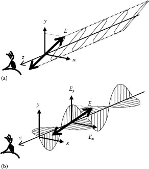
FIGURE 26.1  Electric vector of light. (a) Polarized light and (b) electric vector of light.

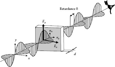
FIGURE 26.2  Electric field before and after passing through a sample.

$\begin{array}{l}{E}_y=A_y\exp i\left(\text{ω}t-\frac{2\text{π}}{\text{λ}}z+{\text{φ}}_y\right)\hfill \\ E_x=A_x\exp i\left(\text{ω}t-\frac{2\text{π}}{\text{λ}}z+{\text{φ}}_x\right)\hfill \end{array}$

(26.1)

provided that the phase difference δ is

$\text{δ\hspace{0.17em}}={\text{φ}}_y-{\text{φ}}_x$

(26.2)

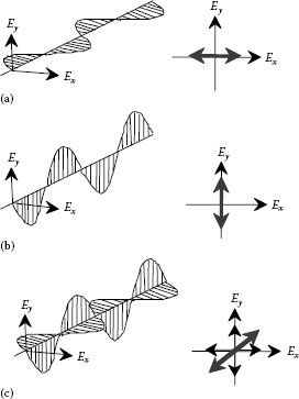
FIGURE 26.3  Composition of the electric vibration vectors E_x and E_y. (a) Linear polarization in case of A_y = 0, (b) linear polarization in case of A_x = 0, and (c) linear polarization A_x = A_y, δ = 0.

It is possible to determine the statuses of linear polarization, circular polarization, and elliptical polarization from the amplitude A and the phase difference δ.

As shown in Figure 26.3, linear polarization takes place when the phase difference is 0 or π. As shown in Figure 26.3a, horizontal linear polarizations vibrating in the x-axis direction are obtained when the amplitude is A_x = 0, vertical linear polarization when A_y = 0 as shown is Figure 26.3b, and linear polarization with azimuth 45° when A_x = A_y = 1, as shown in Figure 26.3, because it is the composition of the amplitude vectors of x and y directions.

Next, circular polarization takes place when δ is 90° as shown in Figure 26.4. In this case, the relationship between the phase differences of E_x and E_y is given as a composition of vectors as shown in Figure 26.4a and traces the locus shown in Figure 26.4c. When observed from the direction of light, the vector’s rotation is counterclockwise as shown in Figure 26.4b, and so the locus will be as shown in Figure 26.4c. Thus, this kind of polarization state is called left-hand circular polarization. In addition, this is when E_y has a phase delay of 90°(–90°) when compared with E_x. On the other hand, if E_y has a phase lead of 90°(+90°), the locus is clockwise as opposed to Figure 26.4. This kind of polarization state is called right-hand circular polarization.

With these facts considered, Equation 26.1 can be expressed as

${\left(\frac{E_y}{a_y}\right)}^2+{\left(\frac{E_x}{a_x}\right)}^2-2\left(\frac{E_y}{a_y}\right)\left(\frac{E_x}{a_x}\right)\cos \text{δ\hspace{0.17em}}={\text{sin}}^2\text{δ}$

(26.3)

Linear polarization is obtained when the phase difference is 0° or 180°. When δ is 90° and A_x = A_y, Equation 26.3 is expressed in the equation of a circle. When the phase difference is anything other than these, the polarization state will have its vectors directed elliptically, and its locus will be as shown in Figure 26.4c. This kind of polarization state is called elliptical polarization.

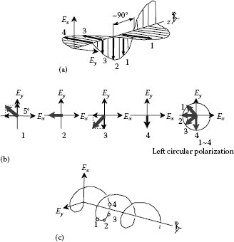
FIGURE 26.4  Left circular polarization light. (a) Polarization state, (b) direction of polarization vector, and (c) trajectory.

26.5    WHAT IS BIREFRINGENCE?

Birefringence has, as it is written, two indexes of refraction. That is, the propagation velocity differs depending on the polarization direction. Figure 26.5 shows how an optical wave transmits double refractive objects with indexes of refraction n_// and n_⊥, respectively. Figure 26.5b separates and aligns vertically each plane of polarization of Figure 26.5a. Phase difference Δ depending on the double refraction occurs between orthogonal polarizations. In Figure 26.5, since light E_x vibrating in the x direction is transmitted through the sample slowly, birefringent phase difference (retardation) depending on the transmitting velocity arises in the light emitted from the sample. In other words, the transmitting velocity in the x direction differs from that in the y direction. That is, their indexes of refraction are different. Since the refractive index is the ratio between the velocity of light c′ transmitted through a substance and the velocity of light c in vacuum,

$n=\frac{c}{c^{\prime }}$

(26.4)

the double refraction Δn is given as

$\Delta n=n_{\perp }-n_{//}$

(26.5)

Generally, birefringent phase difference Δ,

$\Delta =2\text{π}l/\text{λ}\cdot \Delta n$

(26.6)

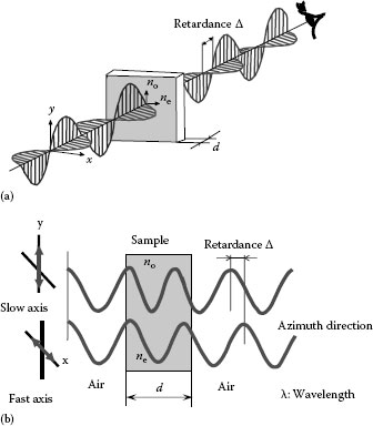
FIGURE 26.5  An example that the light passes though a birefringence sample. (a) Birefringence sample and (b) difference of light speed along the polarization difference refractive index.

TABLE 26.2
Determination of the Retardation Unit

Waves	1 Wave (λ)
Degrees	360°
Radians	2π rad
Nanometers	λ nm
	λ: wavelength

since phase display (2π = 360°) can be expressed as follows:

$\Delta =360\Delta nl/\text{λ}$

(26.7)

and can be standardized by wavelength (nm) in Table 26.2.

The direction in which light is fastly transmitted (phase lead) is called the fast axis. On the other hand, the direction in which light is slowly transmitted (phase delay) is called the slow axis. The general term for the fast axis and the slow axis is the principal axis. In addition, samples with double refraction are called anisotropic and those without double refraction, such as glasses, are called isotropic in optics.

Thus, determination of the size (birefringent phase difference) and the principal axis direction (the fast axis and the slow axis) of a double refraction is needed to measure inner information of a sample.

The s-polarization is called (transverse electric) TE-mode, and p-polarization is called (transverse magnetic) TE-mode.

26.6    NOTATION OF POLARIZATION STATES

The notation of polarization states can be classified into those using visual techniques and those using mathematical techniques. The Poincaré sphere is a visual technique, and the Mueller method and the Jones method are mathematical methods.

26.6.1    JONES VECTOR

To express the polarization state mathematically, let us refer to Equation 26.1, which expresses optical waves decomposed in x and y components. When this equation is expressed in a matrix, it becomes

$E=\left[\begin{array}{c}\frac{A_x}{\sqrt{A_x{}^2+A_x{}^2}}\exp \left(-i\frac{\text{δ}}{2}\right)\\ \frac{A_x}{\sqrt{A_x{}^2+A_y{}^2}}\exp \left(i\frac{\text{δ}}{2}\right)\end{array}\right]$

(26.8)

For, only relative phases should be considered when dealing with general polarization states:

$E=\left[\begin{array}{c}{E}_x\\ E_y\end{array}\right]=\exp i\left(\text{ω}t-\frac{2\text{π}}{\text{λ}}+{\text{φ}}_x\right)\left[\begin{array}{c}{A}_x\\ A_y\exp i\text{δ}\end{array}\right]$

(26.9)

In addition, if the polarization status is the only one to be considered, the amplitude must be standardized. When the phase is also transformed,

$E=\left[\begin{array}{c}{A^{\prime }}_x\\ {A^{\prime }}_y\end{array}\right]=\left[\begin{array}{c}{A}_x\\ A_y\cdot \exp i\left(\text{δ}\right)\end{array}\right]$

(26.10)

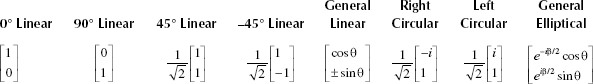
For example, since in horizontal linear polarizations A_x = 1, A_y = 0, and δ = 0, Jones vector J is obtained as follows by using the above equation.

$J=\left[\begin{array}{c}1\\ 0\end{array}\right]$

(26.11)

Also, for instance, in clockwise circular polarizations, A_x = 1, A_y = 1, and δ = 90°. This is when E_y has a lead of 90°(+90°), and Jones vector J is expressed as follows by using the complex number i, the same as the notation of an electric current.

$J=\frac{1}{\sqrt{2}}\left[\begin{array}{c}1\\ i\end{array}\right]$

(26.12)

All polarization states can similarly be expressed with Jones vectors. The Jones vectors of representative polarization states are shown in Table 26.3.

TABLE 26.3
Various Forms of Standard Normalized Jones Vectors

26.6.2  STOKES PARAMETER

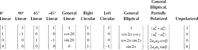
Here, unlike the Jones vector, which uses two elements to express a polarization state, we use the Stokes parameter made up of four elements, s₀ to s₃.

Let us refer to Equation 26.1, which expresses optical waves decomposed in x and y components, just like the Jones vector. When this equation is expressed in matrices, it becomes

$\begin{array}{l}{s}_0=\langle E_x{E}_x^{*}+E_y{E}_y^{*}\rangle =A_x^2+A_y^2\hfill \\ s_1=\langle E_x{E}_x^{*}-E_y{E}_y^{*}\rangle =A_x^2-A_y^2\hfill \\ s_2=\langle E_x^{*}{E}_y+E_x{E}_y^{*}\rangle =2A_x{A}_y\cos \Delta \hfill \\ s_3=i\langle E_x^{*}{E}_y-E_x{E}_y^{*}\rangle =2A_x{A}_y\sin \Delta \text{where}{i}^2=-1\hfill \end{array}$

(26.13)

The four elements could also be expressed with I, M, C, S or I, Q, U, V. When these are put together in the matrix S,

$S=\left[\begin{array}{c}{s}_0\\ s_1\\ s_2\\ s_3\end{array}\right]=\left[\begin{array}{c}I\\ M\\ C\\ S\end{array}\right]=\left[\begin{array}{c}I\\ Q\\ U\\ V\end{array}\right]$

(26.14)

In the Stokes parameter, s₀ stands for the light intensity, stands for the horizontal linear polarization component, s₂ stands for the 45° straight line, and s₃ stands for the right-hand circular polarization. Generally, light intensity is treated as the unit intensity.

Based on these, we deal with representative polarization states. For example, since A_x = 1, A_y = 0, and δ = 0 in horizontal linear polarization,

$S=\left[\begin{array}{c}1\\ 1\\ 0\\ 0\end{array}\right]$

(26.15)

Likewise, in right-handed circular polarization, A_x = 1, A_y = 1, and δ = 90°.

$S=\left[\begin{array}{c}1\\ 0\\ 0\\ 1\end{array}\right]$

(26.16)

All these forms are shown in Table 26.4.

TABLE 26.4
Various Forms of Standard Normalized Stokes Vectors

The relationship between the Stokes parameter’s four elements s₀ to s₃ depends on the polarization state.

In totally polarized lights,

$s_0^2=s_1^2+s_2^2+s_3^2$

(26.17)

In partially polarized lights,

$s_0^2>s_1^2+s_2^2+s_3^2$

(26.18)

Thus, the degree of polarization V is defined as an index of how much light is polarized.

$V=\frac{\sqrt{s_1^2+s_2^2+s_3^2}}{s_0}$

(26.19)

26.6.3    POINCARÉ SPHERE

The possibility of expressing the polarization states mathematically was characteristic to the Jones vector and the Stokes parameter. However, the polarization states, hard enough to perceive, are even more difficult to understand when expressed in matrices. The Poincaré sphere is a method to visually understand the polarization states.

As mentioned in the section dealing with the Stokes parameter, since Equation 26.17 is satisfied in totally polarized lights, when each axis of spatial Cartesian coordinates is expressed as s₁, s₂, and s₃, a sphere with a radius of s₀ is obtained. In addition, if the coordinates of point S, located on the sphere, are expressed with latitude 2β and longitude 2θ, the following equations are obtained.

$\begin{array}{l}{s}_1=s_0\cos 2\text{β}\text{cos}\text{2θ}\hfill \\ s_2=s_0\cos 2\text{β}\text{sin}\text{2θ}\hfill \\ s_3=s_0\sin 2\text{β}\hfill \end{array}$

(26.20)

We will not go into details, but the correspondence to the azimuth θ of the long axis and to the ellipticity angle β in elliptical polarizations can be considered. This situation is illustrated in Figure 26.6. It is easier to understand when the Poincaré sphere is treated as the Earth. A right-hand polarization and a left-hand polarization are created in the upper and lower hemispheres respectively. On the equator, a linear polarization is obtained by the ellipticity of 0°. A right-hand and a left-hand circular polarization are acquired in the upper and the lower poles, respectively, and elliptical polarizations are distributed between each pole and the equator. Polarization states symmetrical about the center of the sphere have a difference of 90° in the azimuth angle of the major axis.

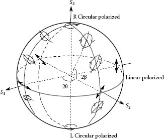
FIGURE 26.6  Poincaré sphere representation of polarization state.

26.7    JONES METHOD AND MUELLER METHOD

All polarization states could be described using the Jones vector and the Stokes parameter. As shown in Figure 26.7, once the incident light and the output light’s polarization states are identified, the polarization elements of an optical device, which is a black box, can be determined subsequently.

The Jones calculus is written as

$\begin{array}{l}J\cdot E=E^{\prime }\hfill \\ \left[\begin{array}{cc}{J}_{xx}& J_{xy}\\ J_{yx}& J_{yy}\end{array}\right]\left[\begin{array}{c}{E}_x\\ E_y\end{array}\right]=\left[\begin{array}{c}{E^{\prime }}_x\\ {E^{\prime }}_y\end{array}\right]\hfill \end{array}$

(26.21)

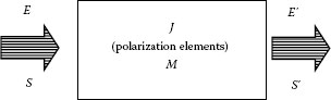
FIGURE 26.7  Jones matrices and Mueller calculus.

The Mueller calculus is indicated as

$\begin{array}{l}M\cdot S=S^{\prime }\\ \left[\begin{array}{cccc}{M}_{00}& M_{01}& M_{02}& M_{03}\\ M_{10}& M_{11}& M_{12}& M_{13}\\ M_{20}& M_{21}& M_{22}& M_{23}\\ M_{30}& M_{31}& M_{32}& M_{33}\end{array}\right]\left[\begin{array}{c}{s}_0\\ s_1\\ s_2\\ s_3\end{array}\right]=\left[\begin{array}{c}{s^{\prime }}_0\\ {s^{\prime }}_1\\ {s^{\prime }}_2\\ {s^{\prime }}_3\end{array}\right]\end{array}$

(26.22)

The polarization elements that can be obtained from these methods are put together in Table 26.5.

Only multiplication of the matrices is needed if the polarization elements are lined together. Additionally, the light intensity obtained at the end in the case of Jones matrix is

$I={\langle E_x+E_y\rangle }^2$

(26.23)

In the case of Mueller matrix, the light intensity is directly given by s₀.

To conclude, the polarization degrees of freedom of the Jones and the Mueller matrices are as shown in Figure 26.7. Both the Jones method and the Mueller method give double refraction, double absorption (dichroism), circular double refraction (optical rotating power), circular double absorption (circular double dichroism), and others.

Their major difference is that as opposed to the Jones vector treating only totally polarized lights, the Mueller matrix can deal with all polarization states including depolarization.

26.8    BIREFRINGENCE MEASUREMENT

26.8.1    LINEAR POLARISCOPE

In this section, we progress to observe and measure stress distribution. Birefringence distribution can be observed from an intensity distribution inserted in a sample between two polarizers as in Figure 26.8. If you analyze this fringe, you can determine the quantity of stress.

In this chapter, three nonmodulated methods and four modulated methods are introduced in the following pages.

Figure 26.9 shows two polarizers and a light source. The optical axes of the polarizer are set perpendicular to each other. A sample is inserted between the polarizers.

The relation among the polarization elements is given using a Mueller matrix and Stokes vector by

$S^{\prime }=P\left(0°\right)\cdot R\left(\Delta ,\text{θ}\right)\cdot P\left(90°\right)\cdot S$

(26.24)

where the Stokes vector S′ and S are the output and input of the light, P(0°), R(Δ, θ), and P(90°) are Mueller matrix of polarizer with 0° of azimuthal direction, sample with Δ retardance and θ azimuthal direction and polarizer with 90° of azimuthal direction, respectively.

The retardance Δ indicates stress-induced birefringence by σ₁ and σ₂.

$\begin{array}{ll}\left[\begin{array}{c}{s}_0\\ s_1\\ s_2\\ s_3\end{array}\right]=\hfill & \frac{1}{2}\left[\begin{array}{cccc}1& 1& 0& 0\\ 1& 1& 0& 0\\ 0& 0& 0& 0\\ 0& 0& 0& 0\end{array}\right]\left[\begin{array}{cccc}1& 0& 0& 0\\ 0& {\cos }^{2}2\text{θ}+{\text{sin}}^{2}2\text{θ}\text{cos}\Delta & \left(1-\cos \Delta \right)\sin 2\text{θ}\text{cos}\text{2θ}& -\sin 2\text{θ}\text{sin}\Delta \\ 0& \left(1-\cos \Delta \right)\sin 2\text{θ}\text{cos}\text{2θ}& {\sin }^{2}2\text{θ}+{\text{cos}}^{2}2\text{θ}\text{cos}\Delta & \cos 2\text{θ}\text{sin}\Delta \\ 0& \sin 2\text{θ}\text{sin}\Delta & -\cos 2\text{θ}\text{sin}\Delta & \cos \Delta \end{array}\right]\hfill \\ \hfill & \times \frac{1}{2}\left[\begin{array}{cccc}1& -1& 0& 0\\ -1& 1& 0& 0\\ 0& 0& 0& 0\\ 0& 0& 0& 0\end{array}\right]\left[\begin{array}{c}1\\ 0\\ 0\\ 0\end{array}\right]=\frac{1}{4}\left[\begin{array}{c}{\sin }^{2}2\text{θ}\left(1-\cos \Delta \right)\\ {\sin }^{2}2\text{θ}\left(1-\cos \Delta \right)\\ 0\\ 0\end{array}\right]=\frac{1}{2}\left[\begin{array}{c}{\sin }^{2}2\text{θ}{\text{sin}}^2\left(\Delta /2\right)\\ {\sin }^{2}2\text{θ}{\text{sin}}^2\left(\Delta /2\right)\\ 0\\ 0\end{array}\right]\hfill \end{array}$

(26.25)

TABLE 26.5
Polarization Elements of Jones Matrix and Mueller Matrix

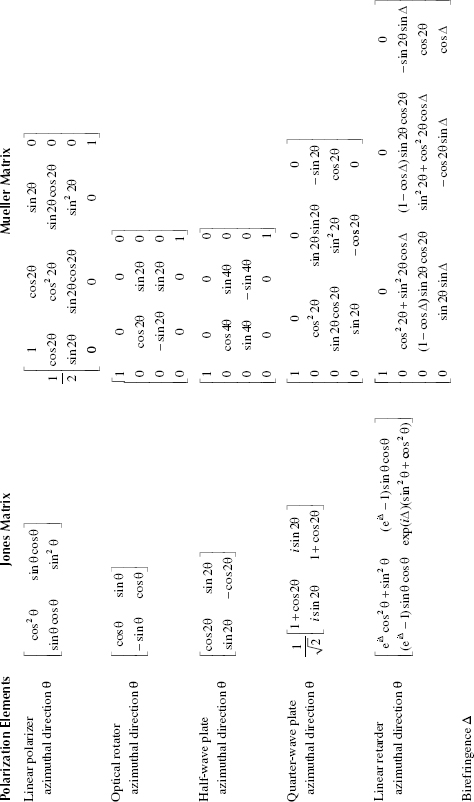
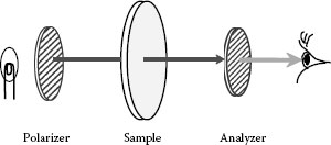
FIGURE 26.8  Visualization of birefringence.

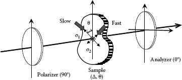
FIGURE 26.9  Plane polariscope.

The intensity I observed at the eye is given from the first term of s₀

$I=s_0=\frac{1}{2}{\sin }^{2}2\text{θ}{\text{sin}}^2\left(\Delta /2\right)=\frac{1}{4}{\sin }^{2}2\text{θ}\cdot \left(1-\cos \Delta \right)$

(26.26)

This means the intensity changes sinusoidally along the retardance Δ and the azimuth angle makes the intensity of the periodic circle 90° independently.

Figure 26.10 shows stress mapping by the plane polariscope [16] (http://www.luceo.co.jp). A plastic disk substrate and square plate are used as samples.

In Figure 26.10a, the intensity distribution of a disk substrate changes bright to dark radially because of the birefringence distribution. The intensity distribution is modulated sinusoidally along the circumferential direction and this period is 90°. This means the azimuth direction of the birefringence indicates concentricity.

The three pictures in Figure 26.10b through d mean merely rotating the sample at the same stress condition. The stress around the surrounding part is larger than that at the center section. This intensity distribution is also modulated sinusoidally in respect of the sample rotation.

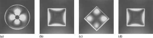
FIGURE 26.10  Stress mapping by the plane polariscope. (a) Plastic disk substrate, (b) stressed plastic plate stress direction is 0°, (c) rotation angle of 45°, and (d) rotation angle of 90°.

It is difficult to determine both the retardance and azimuth direction simultaneously due to the image of the plane polariscope.

26.8.2    CIRCULAR POLARISCOPE

Figure 26.11 shows a circular polariscope. It consists of a circular polarizer and a circular analyzer. A sample is set between quarter wave plates. The relation among the polarization elements is given using a Mueller matrix and Stokes vector by

$S^{\prime }=P\left(0°\right)\cdot Q\left(-45°\right)\cdot R\left(\Delta ,\text{θ}\right)\cdot Q\left(45°\right)\cdot P\left(90°\right)\cdot S$

(26.27)

where

the Stokes vector S′ and S are the output and input of the light

P and Q are Mueller matrix of polarizer and quarter wave plate with azimuthal direction angle between parentheses, respectively

R(Δ, θ) is a Mueller matrix of the sample with Δ retardance and θ azimuthal direction

The retardance Δ indicates stress-induced birefringence by σ₁ and σ₂. All Stokes parameters and Mueller matrices are shown as

$\begin{array}{ll}\left[\begin{array}{c}{s}_0\\ s_1\\ s_2\\ s_3\end{array}\right]=\hfill & \frac{1}{2}\left[\begin{array}{cccc}1& 1& 0& 0\\ 1& 1& 0& 0\\ 0& 0& 0& 0\\ 0& 0& 0& 0\end{array}\right]\left[\begin{array}{cccc}1& 0& 0& 0\\ 0& 0& 0& 1\\ 0& 0& 1& 0\\ 0& -1& 0& 0\end{array}\right]\hfill \\ \hfill & \times \left[\begin{array}{cccc}1& 0& 0& 0\\ 0& {\cos }^{2}2\text{θ}+{\text{sin}}^{2}2\text{θ}\text{cos}\Delta & \left(1-\cos \Delta \right)\sin 2\text{θ}\text{cos}\text{2θ}& -\sin 2\text{θ}\text{sin}\Delta \\ 0& \left(1-\cos \Delta \right)\sin 2\text{θ}\text{cos}\text{2θ}& {\sin }^{2}2\text{θ}+{\text{cos}}^{2}2\text{θ}\text{cos}\Delta & \cos 2\text{θ}\text{sin}\Delta \\ 0& \sin 2\text{θ}\text{sin}\Delta & -\cos 2\text{θ}\text{sin}\Delta & \cos \Delta \end{array}\right]\hfill \\ \hfill & \times \left[\begin{array}{cccc}1& 0& 0& 0\\ 0& 0& 0& -1\\ 0& 0& 1& 0\\ 0& 1& 0& 0\end{array}\right]\frac{1}{2}\left[\begin{array}{cccc}1& -1& 0& 0\\ -1& 1& 0& 0\\ 0& 0& 0& 0\\ 0& 0& 0& 0\end{array}\right]\left[\begin{array}{c}1\\ 0\\ 0\\ 0\end{array}\right]=\frac{1}{4}\left[\begin{array}{c}1-\cos \Delta \\ 1-\cos \Delta \\ 0\\ 0\end{array}\right]\hfill \end{array}$

(26.28)

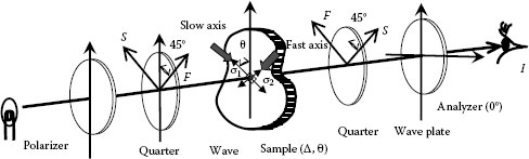
FIGURE 26.11  Circular polariscope.

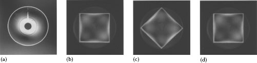
FIGURE 26.12  Stress mapping by the circular polariscope. (a) Plastic disk substrate, (b) stressed plastic plate stress direction is 0°, (c) rotation angle of 45°, and (d) rotation angle of 90° (http://www.luceo.co.jp).

Finally, the intensity I observed at the eye is given from the first term of s₀

$I=s_0=\frac{1}{4}\left(1-\cos \Delta \right)=\frac{1}{2}{\sin }^2\left(\Delta /2\right)$

(26.29)

The intensity distribution means the retardation is changing sinusoidally along the retardance Δ but the azimuth angle is independent of the intensity change.

Figure 26.12 shows stress mapping by the circular polariscope (http://www.luceo.co.jp), the same as that in Figure 26.10.

26.8.3    SENARMONT METHOD

The requirement of birefringence measurement includes stress mapping to measure the state of polarization following the sample, to measure the state of the polarization of incident beam to the sample, or to determine the state of polarization in advance. In addition, it measures the alignment of direction of the sample to incident light or measures both retardation and azimuthal direction. Below are some measurement methods including the Senarmont method, the optical heterodyne method, and the two-dimensional birefringence measurement, using the phase-shifting technique.

The Senarmont method is a classical method for stress mapping. Because it is economical, it is often used for industrial inspection. It has features such as easy alignment, an equal method of ellipsometry, and high accuracy even when using a low-quality wave plate. An optical arrangement of the Senarmont method is shown in Figure 26.13. It consists of a polarizer, a quarter wave plate with 0°, and a rotating analyzer. A sample is set between quarter wave plates with the fixed value of azimuthal direction as 45°. The relation among the polarization elements is given using a Mueller matrix and Stokes vector by

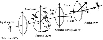
FIGURE 26.13  Optical arrangement of Senarmont method.

$S^{\prime }=P\left(\text{θ}\right)\cdot Q\left(0°\right)\cdot R\left(\Delta ,45°\right)\cdot P\left(90°\right)\cdot S$

(26.30)

where

the Stokes vector S’ and S are the output and input of the light

P and Q are Mueller matrices of polarizer and quarter wave plate with azimuthal direction angle between parentheses, respectively

θ is the azimuthal direction of the analyzer

R(Δ,45°) is a Mueller matrix of the sample with Δ retardance and 45° azimuthal direction

The retardance Δ indicates stress-induced birefringence by σ₁ and σ₂ as shown in Equation 26.11. All Stokes parameters and Mueller matrices are shown as

$\begin{array}{ll}\left[\begin{array}{c}{s}_0\\ s_1\\ s_2\\ s_3\end{array}\right]=\hfill & \frac{1}{2}\left[\begin{array}{cccc}1& \cos 2\text{θ}& \sin 2\text{θ}& 0\\ \cos 2\text{θ}& {\cos }^{2}2\text{θ}& \sin 2\text{θ}\text{cos}\text{2θ}& 0\\ \sin 2\text{θ}& \sin 2\text{θ}\text{cos}\text{2θ}& {\sin }^{2}2\text{θ}& 0\\ 0& 0& 0& 0\end{array}\right]\left[\begin{array}{cccc}1& 0& 0& 0\\ 0& 1& 0& 0\\ 0& 0& 0& 1\\ 0& 0& -1& 0\end{array}\right]\left[\begin{array}{cccc}1& 0& 0& 0\\ 0& \cos \Delta & 0& -\sin \Delta \\ 0& 0& 1& 0\\ 0& \sin \Delta & 0& \cos \Delta \end{array}\right]\hfill \\ \hfill & \times \frac{1}{2}\left[\begin{array}{cccc}1& -1& 0& 0\\ -1& 1& 0& 0\\ 0& 0& 0& 0\\ 0& 0& 0& 0\end{array}\right]\left[\begin{array}{c}1\\ 0\\ 0\\ 0\end{array}\right]=\frac{1}{4}\left[\begin{array}{c}1-\cos \Delta \cos 2\text{θ}-\text{sin}\Delta \text{cos}\text{2θ}\\ \cos 2\text{θ}-{\text{cos}}^{2}2\text{θ}\text{cos}\Delta -\sin 2\text{θ}\text{cos}\text{2θ}\text{sin}\Delta \\ \sin 2\text{θ}-\text{sin}\text{2θ}\text{cos}2\text{θ}\text{cos}\Delta -{\text{sin}}^{2}2\text{θ}\text{sin}\Delta \\ 0\end{array}\right]\hfill \end{array}$

(26.31)

Finally, the intensity I observed at the eye is given from the first term of s₀

$I=s_0=1-\cos \left(\Delta -2\text{θ}\right)$

(26.32)

The intensity modulates sinusoidally along the retardance Δ and the azimuthal direction θ of the analyzer. This means we can determine the retardation Δ from the azimuthal angle θ of the analyzer if we find the dark fringe by the rotating analyzer. The retardation is

$\Delta =2\text{θ}$

(26.33)

26.8.4    PHOTOELASTIC MODULATOR METHOD

One of the popular methods used for many kinds of industries by Hinds is a birefringence measurement system using a photoelastic modulator (PEM) [7,8,9,10]. The optical arrangement consists of a polarizer, a PEM with 0° azimuthal direction, and an analyzer with 0° and 45° azimuthal angle (Figure 26.14). The PEM modulates the retardance δ with temporal modulation. A sample is set between PEM and the analyzer. The relation among the polarization elements is given using Mueller matrices and Stokes vectors by

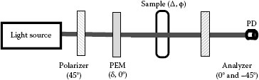
FIGURE 26.14  Optical arrangement of birefringence measurement.

$S^{\prime }=P\left(-45°\right)\cdot X\left(\Delta ,\text{θ}\right)\cdot \text{PEM}\left(\text{δ},0°\right)\cdot P\left(45°\right)\cdot S$

(26.34)

where

the azimuthal angle of the analyzer is 45°

the Stokes vector S′ and S are the output and input of the light, respectively

P is the Mueller matrix of the polarizer

PEM(δ, 0) is the Mueller matrix of the polarizer with the temporal phase modulation δ

X(Δ, θ) is the Mueller matrix of the sample with Δ retardance and θ azimuthal direction

The retardance Δ also indicates stress-induced birefringence by σ₁ and σ₂ as shown in Equation 26.11. All Stokes parameters and Mueller matrices are shown as

$\begin{array}{ll}\left[\begin{array}{c}{s}_0\\ s_1\\ s_2\\ s_3\end{array}\right]=\hfill & \frac{1}{2}\cdot \left[\begin{array}{cccc}1& 0& -1& 0\\ 0& 0& 0& 0\\ -1& 0& 1& 0\\ 0& 0& 0& 0\end{array}\right]\left[\begin{array}{cccc}1& 0& 0& 0\\ 0& {\cos }^{2}2\text{θ}+{\text{sin}}^{2}2\text{θ}\text{cos}\Delta & \left(1-\cos \Delta \right)\sin 2\text{θ}\text{cos}\text{2θ}& -\sin 2\text{θ}\text{sin}\Delta \\ 0& \left(1-\cos \Delta \right)\sin 2\text{θ}\text{cos}\text{2θ}& {\sin }^{2}2\text{θ}+{\text{cos}}^{2}2\text{θ}\text{cos}\Delta & \cos 2\text{θ}\text{sin}\Delta \\ 0& \sin 2\text{θ}\text{sin}\Delta & -\cos 2\text{θ}\text{sin}\Delta & \cos \Delta \end{array}\right]\hfill \\ \hfill & \times \left[\begin{array}{cccc}1& 0& 0& 0\\ 0& 1& 0& 0\\ 0& 0& \cos \text{δ}& \sin \text{δ}\\ 0& 0& -\sin \text{δ}& \cos \text{δ}\end{array}\right]\left[\begin{array}{c}1\\ 0\\ 1\\ 0\end{array}\right]\hfill \end{array}$

(26.35)

Finally, the detected intensity I is given from the first term of s₀

$\begin{array}{ll}I\hfill & =s_0=I_0\left[1+\sin \text{δ}\cdot \left(\cos 2\text{θ}\cdot \text{sin}\Delta \right)-\cos \text{δ}\cdot \left({\text{sin}}^{2}2\text{θ}+{\text{cos}}^{2}2\text{θ}\text{cos}\Delta \right)\right]\hfill \\ \hfill & =I_0\left[1+\sin \left({\text{δ}}_0\sin \text{ω}t\right)\cdot \cos 2\text{θ}\cdot \sin \Delta -\cos \left({\text{δ}}_0\sin \text{ω}t\right)\cdot \left({\sin }^{2}2\text{θ}+{\text{cos}}^{2}2\text{θ}\text{cos}\Delta \right)\right]\hfill \\ \hfill & =I_0\left\{1+\cos 2\text{θ}\cdot \text{sin}\Delta \cdot \left[2J_1\left({\text{δ}}_0\right)\sin \text{ω}t\right]-\left({\sin }^{2}2\text{θ}+{\text{cos}}^{2}2\text{θ}\text{cos}\Delta \right)\cdot \left[J_0\left({\text{δ}}_0\right)+2J_2\left({\text{δ}}_0\right)\cos 2\text{ω}t\right]\right\}\hfill \end{array}$

(26.36)

where J_n is the nth order’s Bessel function.

The phase modulation δ is

$\text{δ\hspace{0.17em}}={\text{δ}}_0\sin \text{ωt}$

(26.37)

where

t is the time

δ₀ is the maximum amplitude of retardance

ω is the angular frequency

Using appropriate modulation δ₀ we can eliminate the J₀ and J₁ terms. If the azimuthal angle θ is 0°, the retardation is obtained using a lock-in amplifier:

$\Delta ={\sin }^{-1}\left[\frac{kI\left(\text{ω}\right)}{J_1\left({\text{δ}}_0\right)}\right]$

(26.38)

In this case, the calibration process is to determine the parameter k.

One more equation is required to determine both retardation and azimuthal direction, simultaneously. The different angles of the analyzer such as 0° are written as

$S^{\prime }=P\left(0°\right)\cdot X\left(\Delta ,\text{θ}\right)\cdot \text{PEM}\left(\text{δ},0°\right)\cdot P\left(45°\right)\cdot S$

(26.39)

The detected intensity I is given from the first term of s₀,

$\begin{array}{ll}{I}_{45°}\hfill & =I_0\left\{1+\sin \left({\text{δ}}_0\text{sin}\text{ω}t\right)\cdot \sin 2\text{θ}\cdot \text{sin}\Delta +\text{cos}\left({\text{δ}}_{\text{0}}\sin \text{ω}t\right)\cdot \left(\left(1-\cos \Delta \right)\sin 2\text{θ}\text{cos}\text{2θ}-\text{sin}\text{2θ}\text{sin}\Delta \right)\right\}\hfill \\ \hfill & =I_0\{1+\sin 2\text{θ}\cdot \text{sin}\Delta \cdot \left[2J_1\left({\text{δ}}_0\right)\sin \text{ω}t\right]\hfill \\ \hfill & -\left(\left(1-\cos \Delta \right)\sin 2\text{θ}\text{cos}\text{2θ}-\text{sin}\text{2θ}\text{sin}\Delta \right)\cdot \left[J_0\left({\text{δ}}_0\right)+2J_2\left({\text{δ}}_0\right)\cos 2\text{ω}t\right]\}\hfill \end{array}$

(26.40)

Using appropriate modulation δ₀ we can eliminate the J₀ and J₁ terms. The amplitude signal of a lock-in amplifier is Δ_0° at the 0° of the analyzer and Δ₄₅° at the 45° of the analyzer. Therefore, retardation is observed by

$\text{θ\hspace{0.17em}}=\frac{1}{2}{\tan }^{-1}\frac{{\Delta }_{45°}}{{\Delta }_{0°}}$

(26.41)

and the azimuthal direction is

$\Delta =\sqrt{{\Delta }_{0°}^2+{\Delta }_{45°}^2}$

(26.42)

Figure 26.15 is a measured result of birefringence distribution of CaF₂ [111]. CaF₂ is only a lens material for UV lithography. A He–Ne laser with 632.8 nm wavelength is used for a light source. The size of material is 40 mm diameter and 7 mm thickness. Retardation distribution is 0.5–7 nm. This distribution is caused by residual stress. If you change a light source to the vacuum ultraviolet such as 157 nm, intrinsic birefringence could be observed.

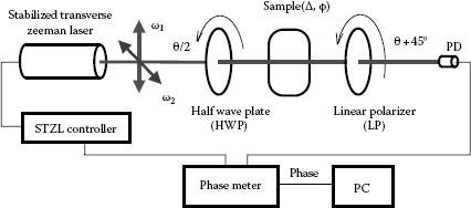
FIGURE 26.15  Optical arrangement of birefringence measurement by optical heterodyne method.

26.8.5  OPTICAL HETERODYNE METHOD

The third method is a birefringence measurement using optical heterodyne detection [10]. Figure 26.15 is an optical arrangement. It consists of a stabilized transverse Zeeman laser (STZL), a half wave plate, and the linear polarizer. The laser STZL has two orthogonal linearly polarized modes and their angular frequencies are ω₁ and ω₂, and ω_b = |ω₁ – ω₂|. The frequency difference is ω_b ≈ 10⁵ rad. The half wave plate and linear polarizer are mounted on a rotating stage. The rotating angle of HWP is 2θ and the polarizer is always 45° between two beams so that they interfere with the sample; when two linear polarizations are aligned with the sample fast axis, the phase shifts one way. About 90° later, the phase shifts in the opposite direction.

The relation among the polarization elements is given using Mueller matrices and Stokes vectors by

$S^{\prime }=L{P}_{2\text{θ}+45}\cdot X_{\Delta ,\text{φ}}\cdot H{W}_{\text{θ}}\cdot S$

(26.43)

The Stokes vector is expressed by

$S=\left[\begin{array}{c}{a}_x{}^2+a_y{}^2\\ a_x{}^2-a_y{}^2\\ 2a_x{a}_y\cos {\text{ω}}_{\text{b}}t\\ 2a_x{a}_y\sin {\text{ω}}_{\text{b}}t\end{array}\right]$

(26.44)

All Stokes parameters and Mueller matrices are shown as

$\begin{array}{ll}\left[\begin{array}{c}{s}_0\\ s_1\\ s_2\\ s_3\end{array}\right]=\hfill & \frac{1}{2}\left[\begin{array}{cccc}1& \cos \left(4\text{θ}-90°\right)& \sin \left(4\text{θ}+90°\right)& 0\\ \cos \left(4\text{θ}+90°\right)& {\cos }^2\left(4\text{θ}+90°\right)& \sin \left(4\text{θ}+90°\right)\cos \left(4\text{θ}+90°\right)& 0\\ \sin \left(4\text{θ}+90°\right)& \sin \left(4\text{θ}+90°\right)\cos \left(4\text{θ}+90°\right)& {\sin }^2\left(4\text{θ}+90°\right)& 0\\ 0& 0& 0& 0\end{array}\right]\hfill \\ \hfill & \cdot \left[\begin{array}{cccc}1& 0& 0& 0\\ 0& {\cos }^{2}2\varphi +{\text{sin}}^{2}2\varphi \cdot \cos \Delta & \left(1-\cos \Delta \right)\sin 2\varphi \cdot \cos 2\varphi & -\sin 2\varphi \sin \Delta \\ 0& \left(1-\cos \Delta \right)\sin 2\varphi \cdot \cos 2\varphi & {\sin }^{2}2\varphi +{\cos }^{2}2\varphi \cdot \cos \Delta & \cos 2\varphi \sin \Delta \\ 0& \sin 2\varphi \sin \Delta & -\cos 2\varphi \sin \Delta & \cos \Delta \end{array}\right]\hfill \\ \hfill & \times \left[\begin{array}{cccc}1& 0& 0& 0\\ 0& \cos 4\text{θ}& \sin 4\text{θ}& 0\\ 0& \sin 4\text{θ}& -\cos 4\text{θ}& 0\\ 0& 0& 0& -1\end{array}\right]\left[\begin{array}{c}{a}_x{}^2+a_y{}^2\\ a_x{}^2-a_y{}^2\\ 2a_x{a}_y\cos {\text{ω}}_{\text{b}}t\\ 2a_x{a}_y\sin {\text{ω}}_{\text{b}}t\end{array}\right]\hfill \end{array}$

(26.45)

Finally, the detected intensity I is given from the first term of s₀

$I={S^{\prime }}_0=a_x{}^2+a_y{}^2-2a_x{a}_y\cos \left[{\text{ω}}_{\text{b}}t-\Delta \cdot \cos \left(4\text{θ}-2\varphi \right)\right]$

(26.46)

where ω_b is called the beat signal of the optical heterodyne method and Δ ≪ 1.

The optical heterodyne technique is one of the famous interferometers, as shown in Figure 26.16. The electric fields with ω₁ and ω₂ are shown in Figure 26.16a. The interference signal at the reference detector and measurement detector are shown in Figure 26.16b and c, respectively. The phase difference in Figure 26.16 means the phase Δ · cos(4θ – 2φ) of Equation 26.46. This retardance Δ and azimuth angle φ are easy to determine by using a discrete Fourier transform. The resolution of the birefringence measurement is 0.01 nm of the retardation at 0.2° of the azimuthal direction.

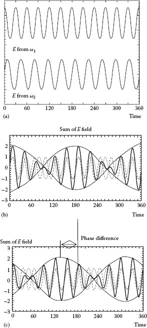
FIGURE 26.16  Optical heterodyne detection. (a) Reference detector measures signal coupled from back of He–Ne laser through LP (45°), (b) from reference detector, and (c) from measurement detector.

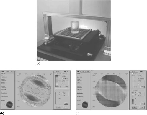
FIGURE 26.17  Stress mapping of CaF₂. (a) CaF₂, (b) retardation, and (c) azimuth direction.

Figure 26.17 is birefringence distribution of CaF₂. The size of this sample is 70 mm in diameter. The distribution of the retardance is less than 25°.

26.8.6    TWO-DIMENSIONAL BIREFRINGENCE MEASUREMENT BY PHASE-SHIFTING METHOD

Figure 26.18 represents a birefringence distribution measurement by the phase-shifting technique [11,12]. Figure 26.18 is an optical arrangement. It consists of a quarter wave plate, a retarder that uses a Babinet-Soleil compensator, and a linear polarizer. A sample with Δ retardation and φ azimuthal direction is set after the retarder. The retarder can work to modulate both retardation δ and azimuthal direction θ.

The relation among the polarization elements is given using Mueller matrices and Stokes vectors by

$S^{\prime }=P\left(\text{θ}+45°\right)\cdot X\left(\Delta ,\phi \right)\cdot R\left(\text{δ},\text{θ}\right)\cdot S$

(26.47)

where

the Stokes vector S′ and S are the output and input of the light, respectively

P is Mueller matrix of the polarizer with azimuthal direction angle θ

X(Δ, φ) is a Mueller matrix of the sample with Δ, retardance and φ azimuthal direction

R(δ, θ) is a Muller matrix of the retarder

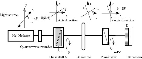
FIGURE 26.18  Birefringence measurement by phase-shifting technique.

All Stokes parameters and Mueller matrices are calculated as

$\begin{array}{ll}\left[\begin{array}{c}{s}_0\\ s_1\\ s_2\\ s_3\end{array}\right]=\hfill & \frac{1}{2}\cdot \left[\begin{array}{cccc}1& -\sin 2\text{θ}& \cos 2\text{θ}& 0\\ -\sin 2\text{θ}& {\sin }^{2}2\text{θ}& -\sin 2\text{θ}\text{cos}\text{2θ}& 0\\ \cos 2\text{θ}& -\sin 2\text{θ}\text{cos}\text{2θ}& {\cos }^{2}2\text{θ}& 0\\ 0& 0& 0& 0\end{array}\right]\left[\begin{array}{cccc}1& 0& 0& 0\\ 0& 1& 0& -\Delta \sin 2\varphi \\ 0& 0& 1& \Delta \cos 2\varphi \\ 0& \Delta \sin 2\varphi & -\Delta \cos 2\varphi & 1\end{array}\right]\hfill \\ \hfill & \times \left[\begin{array}{cccc}1& 0& 0& 0\\ 0& {\cos }^{2}2\text{θ}+{\text{sin}}^{2}2\text{θ}\cdot \text{cos}\text{δ}& \left(1-\cos \text{δ}\right)\sin 2\text{θ}\cdot \text{cos}\text{2θ}& -\sin 2\text{θ}\text{sin}\text{δ}\\ 0& \left(1-\cos \text{δ}\right)\sin 2\text{θ}\cdot \text{cos}\text{2θ}& {\sin }^{2}2\text{θ}+{\text{cos}}^{2}2\text{θ}\cdot \text{cos}\text{δ}& \cos 2\text{θ}\text{sin}\text{δ}\\ 0& \sin 2\text{θ}\text{sin}\text{δ}& -\cos 2\text{θ}\text{sin}\text{δ}& \cos \text{δ}\end{array}\right]\left[\begin{array}{c}1\\ 0\\ 0\\ 1\end{array}\right]\hfill \end{array}$

(26.48)

Finally, the detected intensity I is determined by the first term of s₀

$I=s_0=\frac{1}{2}\cdot I_0\left[1-\cos \left({\tan }^{-1}\left[\Delta \cos \left(2\text{θ}-2\varphi \right)\right]+\text{δ}\right)\right]$

(26.49)

where retardation Δ ≪ 1.

The intensity modulates sinusoidally by changing the phase δ of the retarder in Equation 26.49. If we apply the phase-shifting technique with π/2 of each phase shift shown in Figure 26.19 [13,14], we can determine the initial phase by

$\Delta \cos \left(2{\text{θ}}_M-2\varphi \right)=\frac{I_3-I_1}{I_0-I_2}={\Phi }_M$

(26.50)

The retardation Δ and azimuthal direction φ analytically substitute the phase Φ_M corresponding to the azimuthal angle θ.

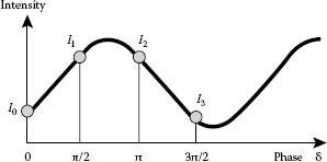
FIGURE 26.19  Four steps of phase-shifting technique.

The birefringence phase difference is given by

$\Delta =\frac{1}{2}\sqrt{{\left({\Phi }_2-{\Phi }_0\right)}^2+{\left({\Phi }_3-{\Phi }_1\right)}^2}$

(26.51)

The azimuthal direction of

$\varphi =\frac{1}{2}{\tan }^{-1}\frac{{\Phi }_3-{\Phi }_1}{{\Phi }_0-{\Phi }_2}$

(26.52)

This means 16 images are enough to determine birefringence mapping. The resolution of retardance is ±1°.

Figure 26.20 shows a birefringence distribution measurement using two LC retarders for highspeed measurement. Three LC retarders are required to determine all polarization states, generally. However, two retarders are enough to determine the limited retardation in this experiment. Two LC cells whose azimuthal directions are set at 0° and 45°, respectively, are used. If the incident light to the LC retarder is circular polarization, phase φ (ellipticity) and azimuthal direction θ by LC retarders are expressed as

$\begin{array}{ll}{\text{δ}}_1\hfill & ={\sin }^{-1}\left(\sin \varphi \cdot \sin 2\text{θ}\right)\hfill \\ {\text{δ}}_2\hfill & ={\tan }^{-1}\left(\tan \varphi \cdot \cos 2\text{θ}\right)\hfill \end{array}$

(26.53)

where δ₁ and δ₂ are retardation of the LC modulator. Figure 26.21 represents a two-dimensional accuracy check using a 15° retarder at three different orientations with 30°, 0°, and −30°. The dots indicate the measurement points, and the directions of the line indicate the azimuthal direction.

Now, a process to determine birefringence distribution of a plastic disk is shown in Figure 26.22. The original image in Figure 26.22a is the same as that of a polariscope. After analyzing the birefringence distribution using 16 images, the birefringence distribution such as retardation and azimuthal angle are shown in Figure 26.22b and c. A vector map shown in Figure 26.22d indicates both magnitude of retardance and azimuthal direction as a whole. A cross section of AA′ in Figure 26.22b is displayed in Figure 26.22e.

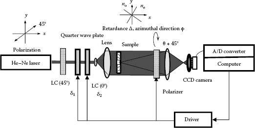
FIGURE 26.20  Birefringence distribution measurement using two LC retarders.

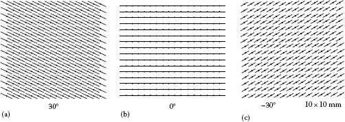
FIGURE 26.21  Two-dimensional accuracy check; same 15° retarder at three orientations. (a) 30° of azimuthal direction, (b) 0° of azimuthal direction, and (c) −30° of azimuthal direction.

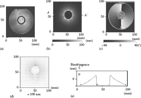
FIGURE 26.22  Process to determine birefringence distribution of plastic disk (3.5 in.). (a) Original image, (b) birefringence distribution, (c) azimuthal angle distribution, (d) vector map, and (e) cross section AA.

This birefringence distribution is mainly caused by polymer orientation. The residual stress mapping of the plastic disk is shown in Figure 26.23. We can compare the affective mapping in Figure 26.23a to the defective one in Figure 26.23b. Both cross sections are shown at the bottom. The birefringence distribution of the defective sample indicates the birefringence change in concentric circles and two parts of the radial direction. The part corresponds to the water channel for cooling water, indicating the residual stress caused by thermal stress.

Figure 26.24 demonstrates stress-induced birefringence by uniaxial stretching. A sample is a gelatin seat measuring 10 × 10 mm. An experimental setup for uniaxial stretching is shown in Figure 26.24a. The stress is indicated by a moving micrometer. Birefringence and azimuthal direction distributions along the length of extension are shown in Figure 26.24b and c, respectively. This relation is shown in Figure 26.25. There are not many changes until 50 ∝m because of the bio-sample [15].

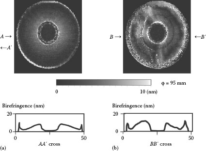
FIGURE 26.23  Plastic disk inspection. (a) Good product and (b) defective product.

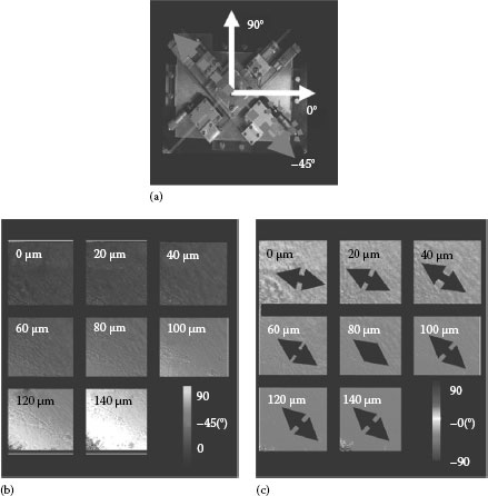
FIGURE 26.24  Change of birefringence under uniaxial stretching. (a) Experimental setup, (b) birefringence distribution, and (c) azimuth distribution.

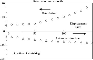
FIGURE 26.25  Change of birefringence under uniaxial stretching.

REFERENCES

1.   P.S. Theocaris and E.E. Gdoutos: Matrix Theory of Photoelasticity, Springer, Berlin, Germany, pp. 105–131, 1979.

2.  R.M.A. Azzam and N.M. Bashara: Ellipsometry and Polarized Light, North-Holland, New York, pp. 153–268, 1987.

3.  D. Goldstein: Polarized Light, Marcel Dekker, New York, pp. 553–623, 2003.

4.  W.A. Shurclif: Polarization Light, Harvard University Press, Cambridge, U.K., pp. 124–148, 1962.

5.  H. Aben and C. Guillement: Photoelasticity of Glass, Springer, Berlin, Germany, pp. 51–77, 1993.

6.  R.A. Chipman: Polarimetry, Handbook of Optics II, Michael Bass (Editor in Chief) McGraw-Hill, New York, Chapter 22, pp. 22.1–22.37, 1995.

7.  Y. Shindo and H. Hanabusa: An improved highly sensitive instrument for measuring optical birefringence, Polym. Commun., 25, 378–382, 1984.

8.  B. Wang: Linear birefringence measurement at 157 nm, Rev. Sci. Instrum., 74, 1386, 2003.

9.  B. Wang and T.C. Oakberg: A new instrument for measuring both the magnitude and angle of low level linear birefringence, Rev. Sci. Instrum., 70, 3847, 1999.

10.  N. Umeda, S. Wakayama, S. Arakawa, A. Takayanagi, and H. Kohwa: Fast birefringence measurement using right and left hand circularly polarized laser, Proc. SPIE, 2873, 119–122, 1996.

11.  Y. Otani, T. Shimada, T. Yoshizawa, and N. Umeda: Two-dimensional birefringence measurement using the phase shifting technique, Opt. Eng., 33(5), 1604–1609, 1994.

12.  Y. Otani, T. Shimada, and T. Yoshizawa: The local-sampling phase shifting technique for precise two-dimensional birefringence measurement, Opt. Rev., 1(1), 103–106, 1994.

13.  J.E. Greivenkamp and J.H. Bruning: Phase shifting interferometry, Optical Shop Testing, Daniel Malacara, (Ed.), John Wiley, New York, Chapter 14, pp. 501–598, 1992.

14.  K. Creath: Temporal phase measurement methods, Interferogram Analysis, David W. Robinson and T. Reid (Eds.), Institute of Physics Publishing, London, U.K., Chapter 4, pp. 94–140, 1993.

15.  M. Ebisawa, Y. Otani, and N. Umeda: Microscopic birefringence imaging by the local-sampling phase shifting technique, Proc. SPIE, 5462, pp. 45–50, (Biophotonics Micro and Nano Imaging, Strasbourg, France), 2004.

16.  Luceo Co., Ltd, Circular polarimetry, http://www.luceo.co.jp/technical/pdf/enhenko.pdf (accessed on January 5, 2015).