
CONTENTS
33.2 Machine-Integrated Encoders
33.3 Checking and Adjusting of Production Machines
33.3.1 Accuracy Assessment of Machine Tools
33.3.3 Adjustment of Repetitively Moving Machine Parts
33.5.1 Automated Visual Inspection
33.6.1 Measurement Uncertainty
33.7 Optical Techniques Frequently Used in Production Metrology
33.7.1 One-Dimensional Techniques
33.7.2 Two-Dimensional Techniques
33.7.3 Three-Dimensional Techniques
33.8 Techniques to Minimize the Effects of Environmental Light
Optical metrology plays an important role in modern production. Numerically controlled (NC) machines and robots depend on encoders for length and angle that are integrated in the respective axes. Optical techniques are applied for checking and adjusting production machines. Robots and automated floor-borne vehicles are guided by optical sensors. Optical techniques are used to check the quality of manufactured workpieces and to establish quality control loops. In the following sections, typical applications will be discussed.
33.2 MACHINE-INTEGRATED ENCODERS
Most NC machines depend on incremental encoders integrated in the linear and rotary axes, and in the majority of cases, these are optical encoders. Incremental encoders render a periodic output signal when the respective axis is moving at constant (angular) velocity. The (angular) distance is determined by adding the periods of this signal. In principle, there are two shortcomings in this technique:
• The measurement is only relative, and an additional reference signal is required to get absolute position data.
• The periodic signal does not reveal the direction of movement.
As can be seen from Figure 33.1, a movement starting from position x1 in the rightward direction gives the same output signal than a movement starting from position x2 in the leftward direction. This ambiguity is solved by using two phase-shifted output signals. A phase shift of π/2 is usually chosen, and the two signals are commonly referred to as sin/cos-signal or quadrature signals. The additional signal B in Figure 33.2 in combination with signal A allows an unambiguous determination of the movement.
Furthermore, it is possible to generate additional signals with precisely determined phase shift as a linear combination of signals A and B, which can easily be performed in real-time by electronic hardware. For sinusoidal signals, the following equation holds:
A number of such phase-shifted copies of the original signals can be used to determine the shift of the object to a fraction of the period of the original signals A and B. Other interpolation techniques make use of phase locked loop (PLL) oscillators that generate a synchronized measurement signal with a multiple frequency. Depending on the S/N ratio of the original signals, interpolation by a factor of 1000 or even more is possible.
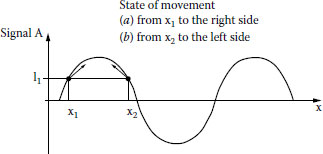
FIGURE 33.1 Ambiguity of direction for a single incremental encoder signal.
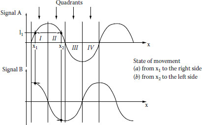
FIGURE 33.2 Unambiguous evaluation of a pair of quadrature signals.
A typical example of a linear optical incremental encoder, the so-called four-field scanning technique, is shown in Figure 33.3. The scale grating is made of glass with a chromium coating that is structured using a precision lithographic process. A common value of the grating period is 20 μm. As this is also the period of the output signal, an interpolation technique is required to get submicron resolution. The scale grating is fixed to the mechanical axis, while a readout head is mounted to the moving slide. This head contains a light source (e.g., an LED), a condenser lens, and several scanning reticles with the same grating period as the scale grating. Moving such a reticle along the scale gives a periodically varying transmitted light intensity. Four reticles are mounted in a way that four phase-shifted signals are generated by the light gathered by the four respective photodetectors. The signals I1,…, I4 can be designated with sin*, cos*, (−sin*), (−cos*). Subtracting (−sin*) from sin* and (−cos*) from cos* cancels the constant background and results in the desired pair of quadrature signals that can be further processed by an interpolation technique. An additional track on the scale grating contains a reference pattern that is read out with a matched reticle to generate the reference signal. When the power is turned on, the axis should first perform a search travel (usually with slow speed), until the reference signal appears. From then on, the absolute position of the slide can be measured by counting the increments of the measurement signal relative to the reference position.
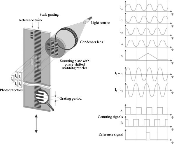
FIGURE 33.3 Linear optical incremental encoder with four-field scanning. (Based on technical information of company Dr. Johannes Heidenhain, GmbH.)
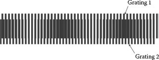
FIGURE 33.4 Moire pattern of the superposition of two gratings with slightly different periods.
In principle, the grating could be directly scanned using photodiodes smaller than the grating period. Using the reticles, however, has several advantages:
• Large photodiodes with a good S/N-ratio can be applied.
• Local defects of the scale or dust have only little effect on the signal quality, because the intensity is integrated over several signal periods.
• While the gratings can only be manufactured with a binary transmission profile, because of the moire effect and diffraction, the signals are nearly sinusoidal, making interpolation easier.
Alternative scanning techniques are available. The single-field scanning technique uses a single scanning reticle with a slightly different grating period. The superposition of two gratings with different period results in a moire pattern with a larger period λbeat, as shown in Figure 33.4.
A linear array of photodiodes is used to read out the moire pattern. These photodiodes are arranged at a distance of λbeat/4 so that their signals can be combined corresponding to the four signals of the four-field scanning technique. Compared to the four-field scanning technique, the larger number of photodiodes and the evaluation of the full width of the grating improve the S/N ratio and make the single-field scanning technique more robust against local defects of the scale grating. Linear encoders based on these or similar evaluation techniques are available with a resolution in the order of 10 nm and an accuracy in the order of 1 μm.
Scale gratings made of glass are limited in length to about 4 m. If longer encoders are required, reflecting scale gratings based on polished steel bands with etched line structures are used. These are manufactured up to lengths of about 30 m. The readout heads are similar to those of the glass scales, but the reflected light is measured instead of the transmitted. Scale gratings made of steel are more robust against vibration and mechanical shocks and their thermal expansion equals that of the machine bed, making thermal compensation easier.
Similar to the linear encoders, angle encoders are based on a radial scale grating with one or more radial scanning reticles. Angle encoders are not only used for the control of rotary axes, but also for linear axes where the rotation of the lead screw is used as a measure of linear movement. While this often is less expensive than a linear encoder, the accuracy is in general worse, because pitch-errors of the lead screw and backlash contribute to the error budget.
For applications with highest demands of accuracy, for example, wafer steppers or ultraprecision machine tools, linear encoders with an interferometric readout scheme are available. In this case, the grating period is in the order of a few micrometers and the scale and the reticle are used as diffraction gratings. Several different diffraction orders are combined and evaluated. A shift of the reticle relative to the scale does not affect the direction of the diffraction orders, but it introduces a phase shift in the diffracted light. This position-dependent phase shift is evaluated interferometrically by the superposition of different diffraction orders, and in that way, a pair of quadrature signals is generated [1].
33.3 CHECKING AND ADJUSTING OF PRODUCTION MACHINES
33.3.1 ACCURACY ASSESSMENT OF MACHINE TOOLS
Machine tools have at least three axes that form their coordinate system, but machines with four or five axes are also widely used. For each linear axis, three deviations of position (x, y, z) and three angular deviations (pitch, yaw, and roll) have to be considered. For each rotary axis, the radial (two directions) and axial run-out, the angle error, and two directions of drunkenness error also add up to six degrees of freedom. In the machine, the deviation of orthogonality of different axes has to be added. Apparently, the determination of the errors of a machine tool is a demanding task.
In practice, usually, a laser interferometer is used to measure linear deviations. Manufacturers of these instruments offer optional optics for the measurement of straightness deviations or small tilt angles. Alternatively autocollimators are applied for the measurement of straightness deviation and tilt angle. Calibrated precision pentagonal prisms are used as a reference for the check of the orthogonality of the axes. These are applicable to both laser interferometers and autocollimators. A detailed discussion of straightness measurement and alignment can be found in Chapter 17.
Since a few years, a self-tracking laser-interferometer is commercially available [2]. This so-called laser tracer is a specially designed laser interferometer that can be rotated in two directions and can be controlled to track a retroreflector moving freely in space. A retroreflecting target is fixed to the moving part of the machine under examination and is simultaneously tracked by at least four laser tracers from fixed positions. Using a multilateration algorithm, the 3D-position of the retroreflector can be calculated. Based on the kinematic model of the machine, the errors of all degrees of freedom of a multiaxes machine can be determined from a set of comparisons of measured versus nominal positions.
A common problem with production machines are vibrations. These cause annoying noise and can deteriorate the precision of the machine. A prerequisite to apply effective countermeasures is the knowledge of the vibration modes and the positions of nodes and antinodes. Vibrations can be measured optically using either laser vibrometers or holographic techniques.
Laser Doppler vibrometers in principle are two-beam laser interferometers. The vibrating surface is used as the reference mirror. If the surface is not specularly reflecting, an imaging lens with large aperture is used to gather the backscattered light. Applying a heterodyne technique, a Bragg cell is used to shift the frequency of the measurement light by a carrier frequency fc. Reflection from a surface moving with velocity v(t) adds a frequency shift of 2v(t)/λ. Usually, the probing beam and the optical axis of the imaging lens are coaxially directed normal to the vibrating surface. v(t) is then the out-of-plane component of the local velocity vector v(t). Superposition of the measurement beam and the reference beam in the vibrometer head gives a beat signal
This can be interpreted as a frequency modulated signal with the carrier frequency fc. It can be demodulated using techniques well known from radio technology. Adding a 2D-scanning optics to such a single point laser vibrometer allows the sequential measurement of the distribution of amplitude and phase of out-of-plane vibration over the surface of an object.
In-plane vibration can be measured by adopting the working principle of laser Doppler velocimetry. Two mutually inclined laser beams are brought to a common focus on the vibrating surface. The focus spot is then structured with a sinusoidal interference pattern with a period depending on the wavelength and the inclination angle of the beams. If there are some inhomogeneities on the surface, the backscattered light will be modulated in intensity, when there is an in-plane-movement orthogonal to the line-pattern; 3D laser vibrometers that combine both techniques to measure the three components of a local velocity vector simultaneously are commercially available.
In contrast to laser vibrometer that scan the surface point by point holographic techniques can be used for integral vibration measurement. In classical holographic interferometry, two main approaches exist: the time-average technique and the double-pulse technique. In both cases, a holographic setup is applied where the coherent light backscattered from the measurement object is superimposed with a reference wave on a photoplate.
For the time-average technique, the exposure time is chosen to be much longer than the period of vibration. If the resulting hologram is reconstructed, a 3D image of the object is visible covered by interference fringes. The contrast of these fringes is highest at the nodes and declines with increasing local amplitude. A double-pulse hologram is taken by using a pulse laser and triggering it at two different states of the vibration, for example, at the two opposite reversal points. In this case, the fringe system covering the 3D image of the object will have constant contrast. As an advantage compared to the time-averaging technique, the double-pulse technique measures not only the amplitude but also the phase of vibration. As a disadvantage the information about the node positions is lost.
In both cases, the distribution of the local amplitude of vibration in the direction of the sensitivity vector, given as the half-angle between the directions of illumination and observation, can be determined with interferometric accuracy. The complete amplitude vector can be measured by combining three setups with noncoplanar sensitivity vector. Holographic interferometry is a powerful tool, but the handling of photographic plates is awkward and time consuming. With the availability of high-resolution electronic imagers and high-power computers, it has been replaced by speckle interferometry and digital holography. Both the time-average technique and the doublepulse technique can be transferred to these new methods. A detailed discussion is beyond the scope of this survey, but can be found in Chapters 7 and 8 and in literature, for example, [3].
33.3.3 ADJUSTMENT OF REPETITIVELY MOVING MACHINE PARTS
There are many applications in production, where precisely synchronized repetitive movements of different parts at high speed are vital, for example, pick and place robots, printing and packaging machines, and automated assembly machines. When it comes to repetition rates of 10 Hz or more and to precision demands of 1/10 mm or less, the analysis of these procedures is beyond the capability of the human eye. In these cases, stroboscopic illumination is a common approach to freeze repetitive movements by illumination with a synchronized flashlight. This can be combined with an electronic camera with short exposure time to get digital images for quantitative evaluation. If a high-speed camera is applied, videos can be taken at a frame rate of 1,000 fps at full frame and more than 10,000 fps at reduced resolution. With this tool, even transient effects can be made visible and measurable. A demanding task, however, is the setting of trigger marks to identify the interesting images in a pile of thousands of images gathered within a few seconds.
The main task of production metrology is the supply of methods of measurement and testing to secure the quality of the manufactured products. In general, it is checked whether certain properties that are vital for the function of a product are lying within given tolerance ranges or not. A simple implementation is the end-of-line test with the aim to identify and reject products that do not meet the specifications (Figure 33.5a).
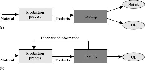
FIGURE 33.5 (a) Product-oriented testing procedure to remove defective products, (b) process-oriented testing procedure; a quality control loop prevents the production of defective products.
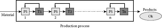
FIGURE 33.6 A chain of quality control loops. Note: PS, production step; T, test.
According to modern production philosophy, however, quality must not be gained by testing, but has to be immanent to the production processes. On each production process, a variety of disturbing influence factors are acting, for example, changing environmental conditions, variations of raw materials, tool wear, limited precision of machines, or human interaction. Production processes, therefore, have to be designed to be robust against these disturbances. Technical systems are made robust by implementing control loops. In a generalized way, production processes are stabilized by implementing quality control loops (Figure 33.5b). The basic difference to product-oriented testing is that the test is not aimed at sorting the products but to get information about the process and, by using a feedback control, make sure to produce only good products. Typical production processes can be separated in one or more chains of production steps. In many cases, these production steps are quality-controlled individually (Figure 33.6). This has the advantages of a faster response and in general less complex inspection tasks compared to the end-of-line test.
Quality inspection tasks can be subdivided into qualitative or quantitative inspection. Only for quantitative inspection, measurements are required. Typical examples of qualitative inspection are the check of the completeness of an assembly and the search for irregularities on a surface (scratches, dirt, dents, etc.). Often these inspections are carried out by human workers, because the tasks may be quite complex and the flexibility and brainpower of humans is still superior to any machine. However, human inspectors cannot guarantee for a continuous high level of quality, because humans tend to get distracted or tired when doing repetitive routine jobs for longer time. On the other hand, the constant reliable operation is a strength of machine vision systems and in many applications, these have been implemented successfully.
33.5.1 AUTOMATED VISUAL INSPECTION
The main components of a machine vision system are at least one electronic camera, an illumination system, a computer hardware, and an image-processing software. Electronic cameras are built around a solid state image sensor, either change-coupled device (CCD) or complementary metal-oxide-semiconductor (CMOS) type. Typical machine vision cameras contain a monochromatic image sensor with a resolution of about 1 Mpixel that is sufficient for most applications and—compared to consumer cameras with more than 10 Mpixels and RGB-color-coded output—reduces the load on interface bandwidth, memory space, and computation power. The pixel size typically is considerably larger than in consumer cameras, resulting in an improved S/N ratio. Most cameras feature an integrated A/D converter and a standardized interface (USB 2.0, USB 3.0 or IEEE 1394a).
The images are evaluated based on the detection of contrast. The most simple case is intensity contrast that can be treated by defining thresholds, either fixed or adaptive. Color contrast is usually transferred to intensity contrast by applying appropriate color filters either in the illumination or in the imaging path. The most difficult task is the evaluation of pattern contrast that requires special image-processing operations like spatial frequency filtering or filters that detect preferred orientations of edges (Figure 33.7).
As a general rule, much effort should be invested in the design of the illumination to enhance the details of interest already in the raw images. Thus, the resulting system will be much more robust and reliable than one depending only on image-processing algorithms. The contrast between different materials often can be enhanced by making use of physical effects. The plastic parts of an electronic board under ultraviolet illumination may look bright against metallic parts because of fluorescence. In other cases, polarized light might be appropriate to enhance the contrast.
A typical example of a high-volume completeness check is the automated optical inspection (AOI) of electronic boards. Because of their flat and regular geometry, the boards can be easily fixed in a well-defined position for inspection. The most simple evaluation is based on a digital reference image of a completely assembled board that is stored in the computer memory. For each serial board, a digital image is taken with an electronic camera under the same illumination conditions and this image is subtracted pixel by pixel from the reference image. A missing component can be easily identified as an object in the difference image.
This simple approach is limited to applications without variations in the components. Some assemblies, for example, a dashboard of a car, may vary in configuration and color from car to car. In such a case, the inspection has to be much more complex. Pattern recognition algorithms are used to identify and localize the different components of the assembly, and the result is compared to the basic schedule of the inspected product.
Human inspectors searching for irregularities on a surface make use of variation of illumination, for example, by looking at the surface from different directions under controlled directed illumination. This approach is adapted by the designers of machine vision systems. Small irregularities on a surface like scratches or dirt are very sensitively detected by using a directed illumination in dark field configuration (Figure 33.8). In case of a perfect surface, the light is reflected past the camera lens, resulting in a dark image. At irregularities, the light is scattered and bright spots or lines are visible in the image. Small dents or waviness on sheet metal on the other hand can very sensitively be detected using directed illumination in bright field configuration and grazing incidence (Figure 33.8). Changes in surface slope are translated to intensity contrast that can be detected automatically in the image.
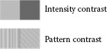
FIGURE 33.7 Intensity and pattern contrast.
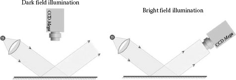
FIGURE 33.8 Different techniques to apply directed illumination for contrast enhancement.
Each workpiece has to fulfill certain requirements, for example, to fit in an assembly. Being aware of the variations unavoidable in every production process, the designer defines not only nominal values for the critical quantities of the workpiece but in addition a tolerance region between a lower and an upper specification limit, LSL and USL, respectively. In quantitative inspection, all critical quantities of a manufactured part have to be measured and the measured value has to be compared to the related tolerance region. However, not only the production process is disturbed by influence factors, but also the measurement process. Therefore, each measurement value may deviate to some extent from the true value.
The measurement deviations can be divided into systematic and stochastic ones. Systematic deviations are repeatable under constant conditions, and therefore, they can be determined by appropriate calibration procedures. Measurement values can be corrected for known systematic deviations, but not for stochastic ones. For these, a statistical analysis is required.
33.6.1 MEASUREMENT UNCERTAINTY
According to the international vocabulary of metrology [4], measurement uncertainty is a nonnegative parameter characterizing the dispersion of the quantity values being attributed to a measurand, based on the information used. The GUM (Guide to the Expression of Uncertainty in Measurement) describes a procedure to systematically identify the parameters that have an influence on the measurement, describe this in a mathematical model, estimate the variation range of the values of all relevant influence factors, and—by applying the mathematical model—estimate the confidence interval, that is, the interval within which the measurement value is to be expected with a probability of 95%. The half-width of this interval is taken as the measurement uncertainty U. The documentation of a complete measurement result always has to include the measurement uncertainty.
In many cases, the tolerance requirements are quite tough and the measurement uncertainty cannot be neglected compared to the width of the tolerance region. In Figure 33.9, a symmetrical tolerance band around a nominal value N is depicted, and it is assumed that the measurement uncertainty has the value U. It is important to be aware that only measurement values between the boundaries (LSL + U) and (USL − U) indicate a workpiece within the specified tolerance limits with a probability >95%. Measurement values within ±U around the specification limits cannot be interpreted with sufficient reliability. Due to the nonperfect measurement process, the width of the tolerance band in effect is reduced by 2U. The investment cost of sophisticated measurement devices with small uncertainty U might therefore be more than compensated by reduced demands on production equipment because of a larger effective production tolerance range.
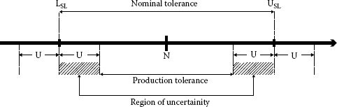
FIGURE 33.9 Reduction of the available tolerance range caused by measurement uncertainty. Notes: N, nominal value; LSL, lower specification limit; USL, upper specification limit; U, measurement uncertainity.
Similar to the process capability index Cp, a measurement capability index Cg has been introduced to evaluate the appropriateness of a measurement process for a given application. It is defined as the width of the tolerance region related to the width of the confidence interval:
In general, only measurement processes with Cg > 5 are considered to be capable.
33.7 OPTICAL TECHNIQUES FREQUENTLY USED IN PRODUCTION METROLOGY
The variety of optical measurement techniques can be arranged according to the dimensionality. Some of the most frequently used techniques are presented in Section 33.7.1.
33.7.1 ONE-DIMENSIONAL TECHNIQUES
A large number of simple devices like light barriers and switching devices are used for counting and checking the presence of workpieces in automated machines.
A very versatile optical distance sensor is the triangulation sensor, shown in Figure 33.10.
The bright spot illuminated by the laser is imaged on a position-sensitive diode (PSD) or a linear CCD image sensor. The distance of the surface is translated to the position of the image of the spot on the sensor. Usually, the sensor is tilted according to the Scheimpflug condition to secure a sharp image within the complete measurement range. Triangulation sensors are available with measurement ranges between 10 mm and 1 m and a relative accuracy of up to 10−5 of the measurement range.
An important task in production metrology is the thickness measurement of continuous products like wire or extruded profiles. A special class of optical instruments applied in this field is called optical micrometer (Figure 33.11). These consist of an illumination unit and a detection unit opposite to one another. The light traveling from the illumination unit is precisely collimated so that the shadow cast by an object keeps its width till it is analyzed by the detection unit. Different kinds of such instruments are available with either continuous illumination or scanned laser beams. If the diameter of the workpiece is large, a so-called optical caliper is built by combining two sensor heads, each detecting one of two opposite edge positions of the workpiece. The diameter is then calculated from both sensor outputs and their distance from one another.
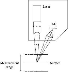
FIGURE 33.10 Triangulation sensor.
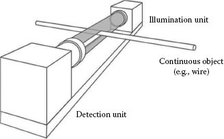
FIGURE 33.11 Optical micrometer.
33.7.2 TWO-DIMENSIONAL TECHNIQUES
For two-dimensional geometrical measurements, usually, electronic cameras are applied. Best contrast of the edges is obtained when using backside illumination. In this case, the workpiece is placed on a glass plate so that no mechanical fixtures are needed. Special instruments incorporating this principle are profile projectors for large- and medium-sized parts and measuring microscopes for small parts. Care should be taken concerning the objective lens, because the accuracy is dependent on its property. Even good lenses show distortion errors of about 10−4; therefore, a calibration of the imaging system is required for precision measurements. Conventional lenses show a distance-dependent magnification factor; therefore, often so-called telecentric lenses are preferred that are designed to have a fixed magnification factor within a certain distance range.
33.7.3 THREE-DIMENSIONAL TECHNIQUES
A variety of optical techniques for three-dimensional measurement are summarized under the term “triangulation.” As a common attribute, all these techniques have at least two optical systems with mutually inclined optical axes. In the case of active triangulation, one of the optical systems is a pattern projector and the other is a camera as shown in Figure 33.12a. Most often, a parallel line grid is projected onto the surface. The surface profile causes a deformation of the pattern when viewed by the camera. The information about the surface is coded in these deformed fringes. Usually, either a sinusoidal pattern is used and a phase-shifting evaluation is applied or the measurement is based on a set of binary line patterns using the Gray-code approach. Details of fringe processing can be found in Chapter 21. Both the optical systems of the projector and the camera have to be calibrated. Two sets of parameters are determined: The parameters of external orientation carry the information about the position and orientation of camera and projector in space. The properties of the two imaging systems are described by their parameters of internal orientation.
Figure 33.12b shows the principle of a passive triangulation setup. In this case, two cameras are combined. If an object point can be identified in both camera images, then its position in space can be uniquely calculated. In this case, the external and internal orientations of the two cameras have to be determined by calibration. Passive triangulation with two cameras is also known as stereo-photogrammetry. Often a pattern projector is also used in passive triangulation. The application of special patterns can make the evaluation procedure easier, faster, and more precise.
The basic difference between active and passive triangulation is that in active triangulation, the projector is part of the reference frame. Because of the light source inside of the projector, it is more likely to be influenced by thermal effects than a camera. The passive triangulation technique therefore has better preconditions for longtime stability and accuracy.
The performance of fringe projection techniques—active as well as passive ones—is strongly dependent on the surface properties of the workpiece. Diffusely scattering surfaces, for example, etched metal, are ideal for these techniques. Many ceramics and plastics are translucent, that is, the light is not scattered from the surface but from somewhere below the surface. Such volume scattering causes deviations in the measured geometry.
Specularly reflecting surfaces on the other hand will reflect the measurement light according to the law of reflection, and only by chance, some reflected rays may enter the camera lens. Transparent surfaces are also not suited for fringe projection, because most of the projected light is transmitted. In practice, reflecting and transparent surfaces are prepared for the application of fringe projection techniques by covering the surfaces with diffusely scattering white powder. But this changes the surface profile slightly, and it causes additional expenditure of work for covering and subsequent cleaning of the surface.
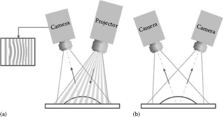
FIGURE 33.12 Basic triangulation setups (a) active triangulation and (b) passive triangulation.
It is a common experience that images generated by curved mirrors show characteristic deformations that carry information about the geometry of the reflective surface. This property is used since long time to check the homogeneity of polished surfaces by looking at the mirror images of line grids. In modern test setups, the grid pattern often is displayed by a flat screen monitor, so that the pattern can be adapted quickly and easily to different testing tasks. This so-called deflectometric technique can be modified to measure the absolute geometry of reflecting and transmitting surfaces. In [5], a correspondence of different deflectometric approaches to the basic principles of active and passive triangulation is outlined.
33.8 TECHNIQUES TO MINIMIZE THE EFFECTS OF ENVIRONMENTAL LIGHT
Many optical measurement instruments like triangulation and light-sectioning sensors, 3D-sensors with structured illumination, speckle-pattern-interferometers, or laser vibrometers depend on the detection and evaluation of light that is projected onto the surface of a workpiece. Any additional light components might disturb the measurement.
While in optical research laboratories experiments can be performed in darkness to prevent erroneous effects of environmental light, optical measurement instruments in industrial applications have to work under varying lighting conditions. Some amount of daylight—dependent on daytime and weather conditions—may be mixed with artificial illumination from incandescent lamps, fluorescent lamps, or LED lamps. In addition, there might be some radiation from hot parts of a machine or the workpiece itself. A number of countermeasures are available to minimize the negative effects of environmental light.
Environmental light sources have to be shielded, when possible. A lens hood can prevent part of the light from entering the optical system. A further reduction of the erroneous light is often possible by inserting baffles into the optical system. In some cases, it is possible to put the complete optical system into an enclosure.
Environmental light most often is unpolarized and spectrally broadband. A considerable reduction of erroneous effects is often possible by making use of a polarized small-band light source for the measurement instrument. A polarizing filter in front of the imaging lens will block the fraction of the unwanted light that is orthogonally polarized to the measurement light. A color filter matched to the spectrum of the measurement light will reduce the effect of broadband environmental light by an order of magnitude or even more. If the interfering light is limited to a certain spectral region, then measurement light from a different spectral region should be applied. A red glowing hot workpiece, for example, would be difficult to measure with a light-sectioning sensor with red laser light. A blue laser diode would give a much better contrast and its light can be extracted easily with an appropriate filter.
Because of their narrow linewidth, lasers are ideally suited for stray light suppression by spectral filtering. On the other hand, their coherent light causes speckle-structures that cause problems in many metrological applications. For camera-based measurement techniques, LED-illumination or spectrally filtered incandescent light therefore is a better choice.
In many optical sensors, the illumination light is electrically modulated, for example, sinusoidally. A matched bandpass filter is applied to the electric output signal to extract the measurement information from the noise caused by the environmental light. The suppression of unwanted signal components is improved with a reduction of the bandwidth of the filter, while on the other hand, the dynamic properties of the sensor are degraded. The S/N ratio of a measurement system with modulated light can be further improved by phase-sensitive filtering (lock-in technique). In camera-based systems, the modulation technique is applied by alternatively taking pictures with illumination switched on and off and by subtracting the adjacent digital images. A combination of shading, optical filtering, and modulation techniques makes optical measurement instruments applicable even under unfavorable lighting conditions.
1. Guan, J. Interferometric encoders for linear displacement metrology, PhD thesis, Technische Universitaet Braunschweig, Braunschweig, Germany, 2013.
2. Schneider, C.T. Lasertracer—A new type of self tracking laser interferometer. Proceedings of IWAA 2004, CERN, Geneva, Switzerland, October 4–7, 2004.
3. Kreis, T. Handbook of Holographic Interferometry: Optical and Digital Methods, Wiley-VCH Verlag GmbH & Co. KgaA, Weinheim, Germany, FRG, 2005. ISBN: 9783527405466.
4. International Vocabulary of Metrology (VIM). ISO/IEC Guide 99:2007, 3rd edn., Beuth Verlag, Berlin, Germany, 2010.
5. Tutsch, R., Petz, M., and Fischer, M. Optical 3D metrology with structured illumination. Opt. Eng. 50 (10), 101507, 2011. doi:10.1117/1.3578448.