
CONTENTS
6.3 Early Examples of Interference
6.7 Twyman Green Interferometer
6.7.1 Mach–Zender Interferometer
6.9.2 Measurement of Materials
6.9.3 Testing of Spherical Surfaces
Interferometry employs the ability of two beams of electromagnetic radiation to interfere with one another provided certain criteria of coherence are achieved. The technique can be used to sense, very accurately, disturbances in one of the beams provided the other beam’s properties are accurately known. There are many variants of interferometers but this chapter discusses the application of interferometers to the testing of optical components and systems, and is restricted to the commonest types of interferometers commercially available.
Interferometry is arguably one of the most powerful diagnostic test tools in the optical toolbox. Interferometric techniques are used for a myriad of purposes ranging from the control of CNC machines of nanometer accuracy to the search for dark matter through gravitational lensing on a cosmological scale. Between these extremes is the use of interferometry in the optical workshop during lens manufacture and system assembly and test, and this subject is the main thrust of this chapter. Interferometers used in optical manufacture range from the very simple, for example, test plates, to the more complex systems used for accurate measurement of components and systems. In common with many other forms of test equipment, interferometric analysis has taken advantage of the developments in computing both in terms of speed and graphical presentation.
The performance of an interferometer depends on the quality of the components used, be they the projecting or collecting optics or the qualities of the radiation source used. The coherence properties of this latter factor are key to the performance of the interferometer both in terms of accuracy and convenience of use.
Interferometers are instruments that can measure directly the distortions of a wavefront resulting from aberrations in optical systems, badly manufactured optical components, inhomogeneities in materials, etc. This is achieved by the measurement of the complex amplitude distribution in an electromagnetic wave. The measurement of the complex amplitude is performed by mixing the distorted wavefront with a nominally perfect wavefront with which it is mutually coherent. Points on the wavefront which are in phase with the perfect wavefront will exhibit a greater concentration of energy than points which are out of phase. The former will thus be bright and the latter dark as shown in Figure 6.1.
The waveforms represent the complex amplitude of the electromagnetic wavefront. The interfering wavefronts are shown as having the same amplitude, so that when they are out of phase by π, there is perfect cancellation. When in phase the complex amplitude of the resultant waveform is double the complex amplitude of the individual waveforms. Note that the time averaged complex amplitude in both cases will still be zero because the electromagnetic wave’s electric and magnetic vectors can take positive and negative values. Fortunately detectors and the human eye do not respond to complex amplitude but to intensity, which as the square of the complex amplitude has the effect of rectifying the waveform. Such detectors then see a time averaged intensity of the rectified waveform; hence the in phase interference will produce a bright area and the out of phase interference a dark area.
Figure 6.2 shows a similar situation except that one of the beams has only half the amplitude of the other. It can be seen that perfect cancellation does not occur so any fringe seen will not have optimum contrast. Additionally the maximum amplitude is reduced. This serves to highlight the need for approximately equal intensity in the interfering wavefronts. A pictorial representation of high- and low-contrast fringes is shown in Figure 6.3.
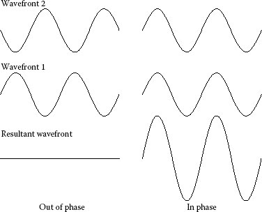
FIGURE 6.1 Summation of complex amplitude.
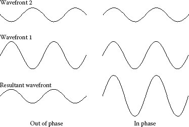
FIGURE 6.2 Summation with non-equal amplitude.
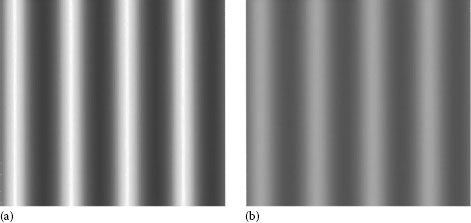
FIGURE 6.3 (a) High- and (b) low-contrast fringes.
Figure 6.4 shows the variation in contrast for different ratios of wavefront intensity. The contrast is defined as
where
Imax is the maximum intensity of the fringe pattern
Imin is the minimum intensity
The contrast is expressed in terms of intensity since that is the condition we can see and detect. Imax is defined by the sum of the amplitudes of the two interfering beams when they are in phase converted to an intensity and time averaged. Imin is the condition when they are out of phase.
The simplest interferometer is simply a plate of glass. The reflectance of the glass will be around 4% from the front and rear surfaces. The setup of such a device is shown in Figure 6.5.
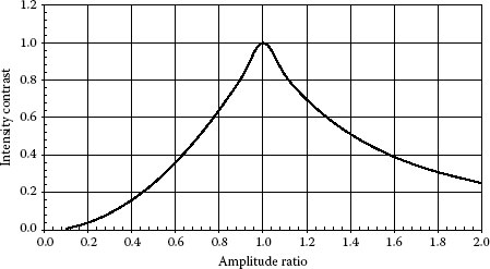
FIGURE 6.4 Contrast for non-equal amplitudes.
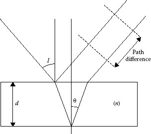
FIGURE 6.5 Two beam interference.
The glass is of thickness d and refractive index n. A plane parallel wavefront is incident on the plate at an angle I. Refraction makes the internal angle different, in this case labeled θ. The path difference between the two wavefronts is given by
or in terms of phase units
where λ is the wavelength of the electromagnetic radiation.
It can be seen that the phase difference between the reflections from the front and rear faces of the glass depends on two parameters that are not single valued. The angle within the plate will depend on the angular subtense of the source. This is normally a pinhole located at the focus of a collimating lens or mirror illuminated by a thermal source. If a screen is placed in the reflected beams then they will produce interference. The phase of the interference will depend on the position within the pinhole from where the particular pair of wavefronts originate. There will effectively be a continuum of interference patterns all of different phase. Since these wavefronts are originating at different parts of a random source, they will not be coherent. This means that all the individual interference patterns will add together in intensity rather than complex amplitude. The result is that the overall contrast is reduced.
If the wavefront from the center of the pinhole is incident normally on the glass plate, then at the center of the beam the path difference between the wavefronts reflected from the front and rear surfaces is
If we now consider a wavefront that originates from the edge of the pinhole, then this will arrive at an incidence angle I. As in Figure 6.5, the angle within the glass plate will be θ. The path difference in this case will be
The change in path difference is given by,
If we assume that θ is small then the expression can be expanded to
If we now consider the wavefronts to have originated at a pinhole of diameter a in the focal plane of a collimator of focal length f, then the maximum angle within the glass plate will be
giving a change in path difference of
As a rule of thumb the maximum shift between the fringe patterns must not exceed a quarter of wavelength (after Lord Rayleigh). Substituting this for ΔP and rearranging gives the maximum value for the angular subtense of the pinhole as
Of course, the corollary is true; if you have effectively zero path difference then useful fringes can be achieved with an extended source. This is the case when optical components are contact tested with test plates. The path length is effectively zero so an extended non-collimated source can be used; normally, a sodium lamp.
Similarly, it is impossible to have a thermal source with zero waveband; there will always be a spread of wavelengths. This has exactly the same effect. Each wavelength produces interference at a different phase, which again reduces the contrast in the fringes. This effect may be reduced by reducing the path difference, so some interferometers which employ relatively broadband sources have a means of introducing phase delay or advancement in one of the beams to ensure that the path difference is as close to zero as possible for all wavelengths. In this way, it is not necessary to define a limiting value as in the case of the pinhole, since the effect may be tuned out, and when it comes to spectral line widths of thermal sources, there is very little that can be done to change it.
Consider the same arrangement as before with a waveband Δλ centered on wavelength λ and normal incidence. At the center wavelength, the path difference, in terms of number of wavelengths, will be
At the extreme of the waveband, the number of wavelengths of path difference will be
If, as before, we make the difference between the two values equal to a quarter of a wavelength, and assuming Δλ is much smaller than λ then after rearranging,
This then describes the maximum bandwidth allowed to achieve interference over a given physical path difference d of index n.
Any departures from flatness of either of the surfaces will lead to a change in the shape of the wavefront reflected from that surface, which will then be evident in the interference fringes. However, the quality of the input wavefront will also have a bearing on the fringe shape. If the input beam wavefront is curved, that is, it is either converging or diverging, then because of the path difference this will show up on the interference fringe.
If the radius of curvature of the input beam is R at the first surface, and the beam is incident normally on the glass plate, then the reflected wavefront will also have a radius R. The beam reflected from the bottom surface will have traversed an additional optical path 2d/n and thus its radius will be R + 2d/n. The curvature of the fringe pattern will be dependent on the difference in the sag of the two wavefronts. If we wished to determine the radius of curvature of one of the reflecting surfaces, these fringes due to the curvature of the input wavefront would be misleading. If it is assumed that we have an aperture of radius h, which is small compared to R, then the sag of the first wavefront is
and that of the second surface is
If we then specify a minimum value that this change should be in order to satisfy the measurement accuracy required,
And assuming that d is much smaller than R, then a minimum value of R can be calculated as
If we take a typical case, most visible interferometers have an aperture of 0.1 m, the propagation is in air and the wavelength is 632.8 nm. To produce a wavefront error of 0.05λ with a propagation distance of 1 m, the radius of curvature of the input wavefront should be 281 m. To make measurements of this order of accuracy, then the error on the wavefront must be significantly less than this, an order of magnitude improvement is generally assumed.
As we shall discuss later, with the advent of software analysis this is not the problem it once was, since software, particularly phase-shifting software, can be calibrated to remove any artifacts due to the quality of the input wavefront.
Another possible area of error is with the collecting optics. Typically this will be an achromatic lens. If the test requires that the operator input a large number of tilt fringes, then the two interfering beams can take different paths through the collecting optics. If the optics are poor, then the aberrations will be imprinted onto the two wavefronts. However, with different paths taken, it is possible that the two beams will suffer differently. An example is if the lens suffers from spherical aberration. A wavefront aberration will be introduced into both the test and reference beams dependent on the position in the pupil of the collection lens.
For the test beam, considering only the direction of tilt
For the reference beam
This latter equation may be expanded to
We assume that powers of δy greater than 1 can safely be ignored. If we now look at the additional apparent aberration introduced into the test beam,
this has the appearance of coma. The aberration does not exist in the item under test, but is introduced by the failure of the collecting optics to properly handle the pupil shear caused by introducing tilted fringes.
6.3 EARLY EXAMPLES OF INTERFERENCE
Several very simple experiments were performed to demonstrate the principle of interference of electromagnetic radiation. Although seemingly simple now, at that time they were groundbreaking experiments. The aims of the experiments were to demonstrate that interference could take place and hence demonstrate that light behaves as wave rather than a particle. Modern quantum mechanics tells us that the picture is much more complex than the simplistic view taken at the time and that the photon can paradoxically demonstrate wave and particle characteristics.
Perhaps the simplest arrangement was devised by Young. This comprised a light source, two slits and a screen (Figure 6.6). The slits were narrow enough such that the light would diffract into a cone.
In the shaded region, where the two cones overlap, straight-line fringes are seen.
Other experiments are variations on the above theme. Fresnel achieved interference using an optical component, a biprism, as shown in Figure 6.7. In this case, the manipulation of the beam, to provide two overlapping beams, is performed using refraction rather than diffraction. Energetically this is a much more efficient system.
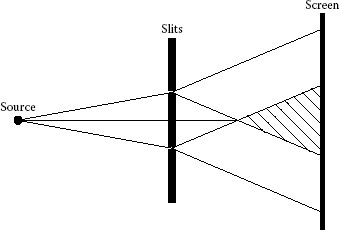
FIGURE 6.6 Young’s slits.
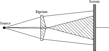
FIGURE 6.7 Fresnel biprism.
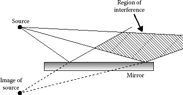
FIGURE 6.8 Lloyd’s mirror.
Another version uses reflection to split the beam into two. This is Lloyds experiment and is shown in Figure 6.8.
Traditionally, the sources used in interferometers have been arc lamps, which display a strong narrowband emission line such as sodium or mercury lamps. As described above, the performance of the interferometer will depend on the narrowness of the emission line and the size of the source. The source size is normally controlled by a pinhole so some optimization is available by reducing the pinhole diameter but at the cost of reducing the amount of illumination available for viewing and recording.
In recent years, lasers have been exclusively used in commercially available interferometers. In particular, the helium–neon (HeNe) laser operating at 632.8 nm is extensively used for testing of glass optical components and systems. The laser has a much narrower spectral bandwidth than thermal sources and thus has a much longer coherence length; rather than the millimeters of path difference permitted, useful interference fringes can be obtained over path differences of many meters. Lasers do, however, have their own problems. In particular, because of the very long coherence length, the unwanted returns from scattering and reflecting surfaces other than those intended can also give unwanted fringes in the final image. These tend to be of much lower contrast than the intended interference fringes and can normally be accounted for.
A greater problem is the stability of the laser cavity itself, coupled with the fact that many lasers will emit several longitudinal modes at the same time. Because of the nature of the cavity design, wavefronts separated by one cavity length will be in phase, because the ends of the cavity represent nodes in the wavefront and this will be true of each longitudinal mode. Outside the cavity, any single mode will interfere with copies of itself produced by reflections representing long path differences. When multiple modes are present, then each mode will produce an interferogram, which has a different phase to the others. However, because of the nature of propagation within a cavity, all these interferogram will be in matched phase at intervals equivalent to multiples of the cavity length. The result is that good contrast fringes may be achieved by tuning the path difference to a multiple of the cavity length. It is safest to use a single-mode stabilized laser; however, this can come at significantly increased cost, and depending on the wavelength chosen can be difficult to procure commercially.
The best laser that the author has used for interferometry has been at 10.6 μm using a CO2 laser. These are generally single-mode devices and can produce high contrast fringes over many tens of meters. On the other hand, at 3.39 μm a HeNe laser is used. At about 1 m long, this laser will produce either two or three modes within the gain bandwidth of the cavity, the number often varying with temperature. When operating in three modes, the central mode is dominant and good contrast fringes can be achieved over many meters. When operating in two modes, they have roughly equal power. Both modes will produce interference fringes, but at intervals along the axis, the two sets of interference fringes are exactly out of phase and cancel out each other. Midway between these positions, the two interference patterns have the same relative phase and thus add together. These lasers often need several minutes to achieve a steady temperature so that there is no thermal mode hopping. The cavity length is then tuned for the environment to produce a dominant longitudinal mode. The lasers are then stable over long time durations.
In recent years, advances in the quality of laser diodes, have made them suitable for long path difference interferometry, though it is often necessary to spatially filter the laser, usually by transmitting it through a single-mode optical fiber. Laser diodes have been used at 850 nm and 1.55 μm, very successfully with path differences of several meters.
Figure 6.9 demonstrates the method that is employed to achieve the interference fringes. An incoming beam of monochromatic radiation is split into two at a beam splitter. In the example shown, part of the beam is retroreflected (we will call it “R”) and part is transmitted “T.” The reflected component R propagates directly toward the detection system. The transmitted beam T carries on toward the optical system under test, in this case a simple reflector, and is retroreflected back through the optical system toward the beam splitter. In this case the surface under test also performs the retroreflection. Part of the beam passes through the beam splitter where it is free to interfere with the original component R. The probe or test beam effectively passes through the component under test twice, thus the system is said to be a double-pass interferometer in which the apparent aberrations are doubled. The separation between adjacent bright areas in the interference pattern thus represents λ/2 of aberration. In this way, a useful doubling of sensitivity can be achieved.
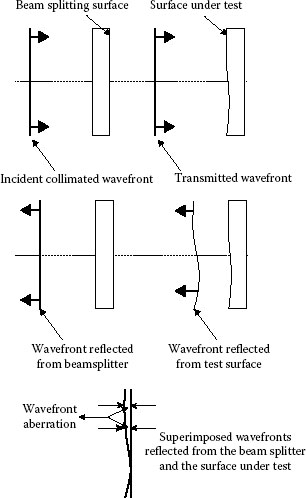
FIGURE 6.9 Simple interferometry.
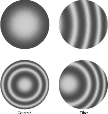
FIGURE 6.10 Interference fringes of a curved wavefront.
The reflected beam from the beam-splitting surface may be tilted by tilting the beam splitter in order to introduce tilt fringes that can help to clarify the aberration shape for small aberrations. Figure 6.10 shows an example of how this can be of use.
The centered (Figure 6.10a) interferogram cannot be reliably assessed because it cannot be determined what proportion of a fringe the variation in intensity represents. By introducing tilt fringes as in tilted (Figure 6.10a), then a measurement is possible.
When there are a large number of fringes as in Figure 6.10b, then information may be obtained from both centered and tilted fringe patterns. In severe cases it may not be possible to remove the central closed fringe from the pattern without introducing so many fringes that visibility becomes a problem.
Figure 6.11 shows the optical arrangement of a Fizeau interferometer. This is one of the simplest arrangements. In the above form, however, it does have certain limitations, in that for thermal sources the spectral lines are not sufficiently narrow to provide a very high level of coherence, thus the beam-splitting surface must be close to the surface under test. This makes it difficult to test complete optical systems. Additionally, in the infrared (IR), thermal sources are not available with sufficient intensity to stimulate a sensor such as a pyroelectric vidicon, which is relatively insensitive. More sensitive sensors are expensive and require cooling. The arrangement shown in the figure is only slightly more sophisticated than using optical test gauges in a polishing shop.
This problem is solved by substituting a laser for the thermal source (Figure 6.12). We now have a long coherence length that will enable much more complex systems to be tested, and we have an abundance of power to stimulate the sensor. For systems employing CO2 lasers, the problem is usually one of how to remove much of the laser power before it impinges on the sensor. Great improvements in the sensors, particularly focal plane arrays, have meant that much less laser power is required to produce good quality images. At most, a few tens of milliwatts are needed in the IR. Visible systems typically have 5 mW HeNe lasers.
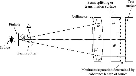
FIGURE 6.11 Fizeau interferometer.
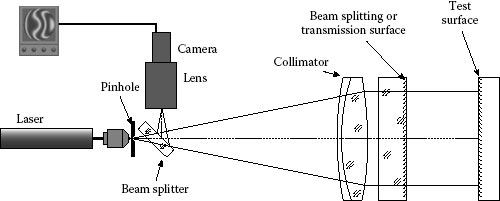
FIGURE 6.12 Laser Fizeau interferometer.
The use of lasers does have a disadvantage in that the long coherence length enables interference to take place between any of the many beams that are reflected around an optical system due to imperfections in coatings and the like. For this reason it is necessary to be very careful regarding antireflection coatings on all optical components after the pinhole. The pinhole itself acts as a spatial filter for all optics that precedes it and thus removes all coherent noise from focusing optics such as microscope objectives used in visible or near-IR systems.
The Fizeau arrangement has one major advantage over other optical arrangements—that all of the optical system of the interferometer is used identically by both the test beam and the reference beam, except for the single surface that performs the beam splitting. This means that aberrations in the interferometer optical system only have a low order effect on the shape of the fringe pattern ultimately observed. The beam-splitting surface, however, must be of very high quality to avoid having a major effect on fringe shape.
In order to measure non-flat surfaces, the beam from the interferometer must be modified using a transmission sphere as shown in Figure 6.13. The beam from the interferometer is collimated as usual, but a lens is affixed to the front of the interferometer. This focuses down with a f/number suitable for testing the component for test. The final surface of the transmission sphere is concentric with the focus of the transmission sphere so that the rays of light are incident at normal incidence. This surface is uncoated so that a reflection is obtained back into the interferometer—this represents the reference beam. The reflectivity of the surface under test must be similar in order to obtain high contrast fringes. Tilt is normally introduced by tilting the whole transmission sphere. Interferometers normally have a range of transmission spheres with different f/numbers, which enable the optimization of test arrangements.
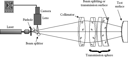
FIGURE 6.13 Testing of spherical surfaces.
6.7 TWYMAN GREEN INTERFEROMETER
Another very common type of interferometer used in optical laboratories and workshops is the Twyman Green interferometer (Figure 6.14). When using a thermal source such as a mercury lamp, this arrangement has significant advantage as the lengths of the two arms can be equalized by mounting the reference mirror on rails and moving it. Until the advent of laser sources in interferometers, this system was very widely used for the assessment of complete optical systems in preference to the Fizeau interferometer, which with a thermal source has very limited application. Using laser sources, this system can still be used effectively; however, the number of components that must be made to high accuracy increase. Both sides of the beam splitter, together with the reference mirror, now need to be very flat. The optics used for collimating the laser beam and for projecting the combined beams to the camera need not be accurate to the same extent.
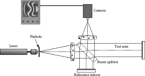
FIGURE 6.14 Twyman Green interferometer.
6.7.1 MACH–ZENDER INTERFEROMETER
The Mach–Zender interferometer is shown in Figure 6.15. This is different from the interferometers already shown in that the test and reference arms take completely different paths.
The Mach–Zender is a single-pass interferometer; the two beams are recombined after the test beam has passed through the optical system under test. The advantage of this over the double-pass interferometer is that apertures that may cause diffraction are only passed once, thus it is much easier to focus on the diffracting aperture to remove the effects of diffraction. This type of system is invaluable in situations where diffraction is important, such as the testing of microlenses.
Figure 6.16 shows a shearing interferometer consisting of a single plate of glass. This duplicates the optical beam complete with any defects it has picked up after passing through an optical system. The two beams are then interfered with one another. This is equivalent to differentiating the wavefront in the direction of the shear.
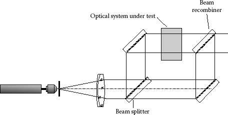
FIGURE 6.15 Mach–Zender interferometer.
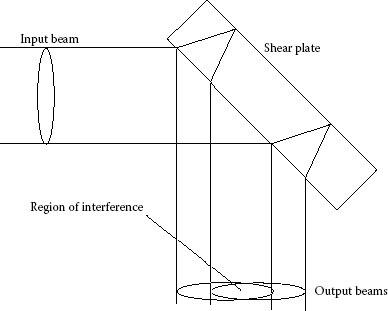
FIGURE 6.16 Shear plate interferometer.
Considering an incoming beam with a focus defect, then the wave aberration is described as
The other pupil is displaced by an amount δy so that its aberration is from a slightly different part of the wavefront.
The resulting fringe pattern represents contours of wavefront given by
or
This is linear with y, so a defect of focus in the input beam will produce straight-line fringes. The spacing of the fringes will depend on the amount of defocus and the amount of shear between the two pupils.
This type of interferometer is very useful for focusing optical systems, in particular collimating systems for other interferometers. Because the fringes are straight, it is very important that there are no other sources of straight-line fringes in the shear plate, that is, the two faces must be parallel to one another.
Interferometry is used as a routine test for optical components and systems at wavelengths ranging from the visible to above 10 μm. In the IR, the main wavebands used are from 3 to 5 μm and from 8 to 12 μm. Typical laser sources used are HeNe (3.39 μm) and HeXe (3.49 μm) in the shorter waveband. CO2 lasers (10.6 μm or tuneable) are used in the longer waveband. IR interferometry presents some problems that require that special care is taken in the setting up of the measurement, and that the results are analyzed in as rigorous a manner as possible.
Infrared optical systems are being produced with smaller optical apertures than previously for reasons of weight, cost, and configurability. This trend has been aided by improvements in the detector technology. The result is that the IR lens for a camera system may have an aperture comparable in size to a visible camera system. However, the wavelength in the IR system may be as much as 20 times greater than in the visible band. This makes the effects of diffraction much more dominant in IR interferometry, requiring that optical pupils are well focused onto the interferometer’s camera sensor surface. Because of the double-pass nature of most commercially available interferometers the aperture is “seen” twice by the interferometer—if the two images of the optical aperture are not conjugate with one another, then some diffraction is inevitable. The effects of this must be minimized to enable accurate analysis.
Figure 6.17 shows two ways of analyzing a lens with an interferometer. One test uses a spherical reference mirror while the other uses a flat reference mirror but requires an additional high-quality focusing lens (or reference sphere) in order to make the measurement. From the point of view of diffraction, the measurement using the reference sphere is preferred since the return mirror can be very close to the pupil of the lens under test, and therefore the pupil and its image via the mirror can both be very close to the focus on the interferometer’s camera faceplate. This is not possible using the other arrangement, diffraction will be present especially if the spherical mirror radius is small so that it is physically far from the lens under test. Many tests in the IR use high grade ball bearings as a return mirror—it is important that any analysis of the interferograms takes into account the limitations of the method.
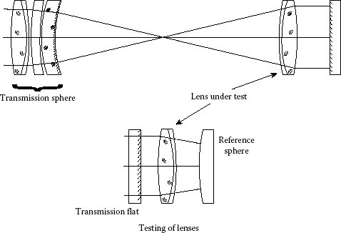
FIGURE 6.17 Reflection configurations.
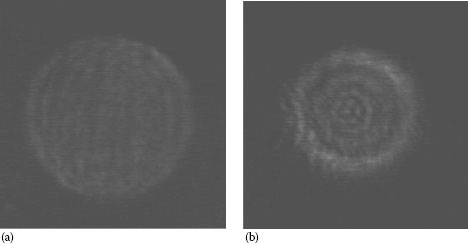
FIGURE 6.18 Pupil imagery. (a) Focused and (b) unfocused pupil.
Figure 6.18 shows the effect of diffraction on the pupil imagery in the interferometer. In the unfocused case, diffraction rings can clearly be seen inside the pupil. This has the effect of breaking up the interference pattern such that the fringes are discontinuous or vary in width due to contrast changes. Any automatic fringe analysis program must be used with caution when analyzing such fringes. In general, the peak-to-valley wavefront aberration reported will be worse than the actual for the lens under test.
While Figure 6.18 shows the effect of diffraction within the optical pupil, the other common case is when the diffracted radiation appears outside the pupil. This has the effect of blurring the pupil edge and so its size is uncertain and because the diffracted radiation has a different curvature to the main beam, any interference fringes will curve within this zone. The effect is very similar to that seen with spherical aberration especially that of higher order and if not corrected can lead to a large departure in measured versus actual performance. This situation is shown schematically in Figure 6.19.
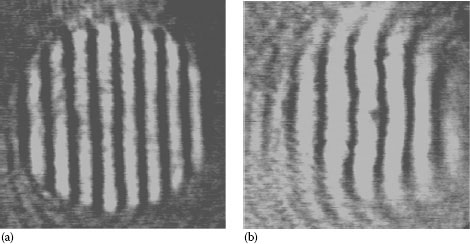
FIGURE 6.19 Pupil imagery effects on fringes. (a) Focused and (b) unfocused pupil.
In this case, if information is known about the size of the pupil within the interferogram, it is possible to mask out much of the effects of diffraction simply by ignoring those parts outside the pupil.
There will be cases where it is impossible to achieve good pupil imagery without going to great expense. In such circumstances, double-pass interferometry can still provide a confidence test on system performance, but ultimate proof may require a single-pass test, either by interferometry or by noncoherent broadband modulation transfer function (MTF) testing or similar.
Infrared interferometry relies on sensing using an IR camera, either staring array cadmium mercury telluride (CMT) or a pyroelectric vidicon tube. The cameras exhibit random noise on the video signal. This is most obvious in the 3–5 μm waveband, where available, affordable lasers tend to be of low power (typically 5–10 mW). High signal gain is required to provide sufficient contrast for recording fringe patterns or analyzing fringe patterns using either static or phase-shifting software. It is also of relevance when laser power is marginal is the profile of the laser beam. As much of the beam as possible must be used to maximize contrast but this does mean that, due to the profile, the contrast varies across the interferogram. This is particularly noticeable when using HeNe lasers at 3.39 μm where perhaps only 5–10 mW of power is available. This can have the effect of making fringes appear both fainter and thinner toward the edge of the pupil. When using static fringe analysis packages, care needs to be taken to check that the digitized fringes accurately represent the real shape of the fringe pattern.
The problems raised by laser power profiles are greater when using phase-shifting systems. Phase-shifting systems involve a threshold contrast below which phase will not be measured. This normally shows as a blank space in the resulting phase map. This can be remedied by reducing the threshold. However, using pyroelectric vidicons with marginal laser power represents a very noisy environment. Reducing the threshold too far means that the system can pick up on random noise in the picture and allocate phase values that are significantly larger than any other area of the pupil. This has the effect of a gross distortion of the results. A fine balance needs to be trodden between these two situations such that phase information is available over the whole pupil without random noise causing a problem. Generally with 3.39 μm systems, the threshold needs to be set at around 2.5%–3.5%.
At 10.6 μm, these problems do not occur. The main problem in the upper IR waveband is finding ways of dumping excess energy. This is normally performed with CaF2 filters. At 10.6 μm 4 mm thickness of CaF2 will absorb 75% of the radiation. With tuneable systems a wire grid polarizer is necessary since the CaF2 does not absorb so strongly at the shorter wavelengths. Because so much power is available, the central part of the beam can be used ensuring a much flatter profile, and sufficient power can be allowed through in order to enable the camera to be set to low gain, thereby reducing noise to an insignificant level.
We have already seen how a single flat optical surface can be measured using an interferometer. Other surfaces, components, and systems often require some specialized equipment in addition to the interferometer. These will include transmission spheres, which are high-quality lenses used to condition the beam from the interferometer so that it can be focused in the focal plane of a lens or system of lenses; beam expanders, which enable the size of the test beam to be enlarged to accommodate larger optical apertures; and attenuators, which allow an operator to match the amplitudes of test beams and reference beams thereby maximizing fringe contrast.
A simple arrangement for testing flats is shown in Figure 6.20. The flat for measurement simply replaces the return mirror. The reference beam arises from the transmission flat that is shown mounted in a tilt stage, which permits horizontal and vertical tilt fringes to be introduced.
6.9.2 MEASUREMENT OF MATERIALS
An arrangement for measuring materials is shown in Figure 6.21. The material is simply placed within the test arm. Various properties of the material can produce distortions of the fringe pattern, these being departures from flatness of the two surfaces and inhomogeneity of the refractive index of the material. Before the advent of highly accurate phase-shifting interferometers, in order to assess the homogeneity of a material, the two sides of the material blank had to be polished very flat such that they would not contribute to fringe distortion. Modern systems can measure the homogeneity of materials by combining a number of measurements which record the total fringe distortion of the blank combined with individual measurements of the two surfaces.
6.9.3 TESTING OF SPHERICAL SURFACES
Concave surfaces are measured by using a transmission sphere focused down at the center of curvature of the concave surface (Figure 6.22).
Convex surfaces are shown in Figure 6.23. It is immediately obvious that there is a significant problem with the measurement of convex surfaces. In order to measure the surface, the output optical aperture of the transmission sphere must be greater than the diameter of the spherical surface under test. It is often necessary to expand the beam from the interferometer so that a larger diameter transmission sphere can be used. Convex surface do not suffer from this problem since the transmission spheres focuses through the center of curvature so that as long as the f/numbers of the transmission spheres and surface under test are matched, the whole surface can be covered.
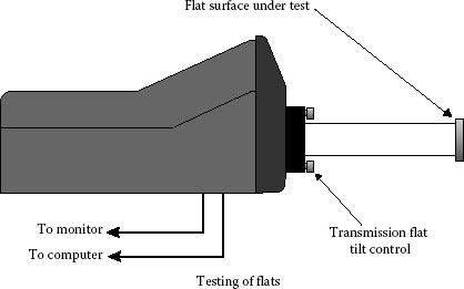
FIGURE 6.20 Testing of flats.
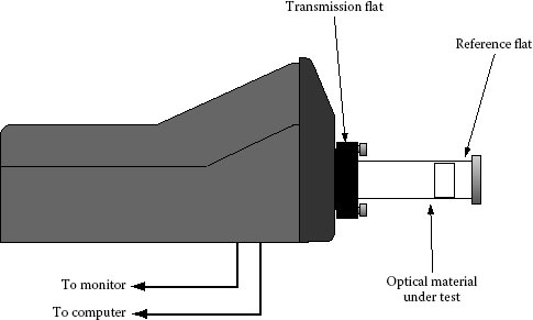
FIGURE 6.21 Testing of material blanks.
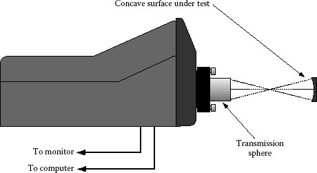
FIGURE 6.22 Testing of concave surfaces.
Figure 6.24 shows the arrangement for testing a lens. The transmission sphere focuses at the focus of the lens under test. A flat return mirror is then used to reflect the radiation back into the interferometer.
A common component in surveillance systems and aerial photography is a protective dome behind which the camera is free to move so that it can be pointed. The test arrangement for such a component is shown in Figure 6.25. A high-quality convex return mirror is used to return the radiation to the interferometer.
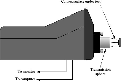
FIGURE 6.23 Testing of convex surfaces.
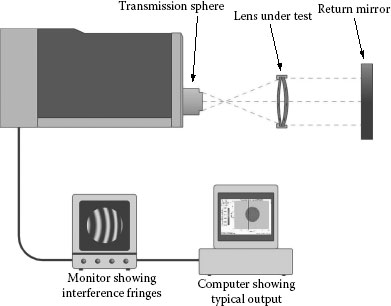
FIGURE 6.24 Testing of lenses.
The testing of a telescope is shown in Figure 6.26. The telescope being afocal can be measured from either direction with a collimated beam. The configuration shown has obvious advantages in that the table area required to perform the measurement is small and the relative cost of the mounting and optical components required when compared with large aperture systems is also reduced. However, there are other advantages with regard to pupil focusing at high magnifications. The effective depth of focus for the pupil imagery can be large in this arrangement thereby reducing the effects of diffraction. For low magnification system or systems where the return mirror is placed at the eyepiece end, the positioning of the return mirror with respect to the position of the entrance pupil becomes much more important.
Telescopes often have zoom or switched magnification arrangements. It is often found that at the high magnifications the optical pupil of the telescope is near the front lens. At the smallest magnification, the pupil is often buried within the telescope. This makes it impossible to focus the optical pupil efficiently for all magnifications and some diffraction effects are likely to occur.
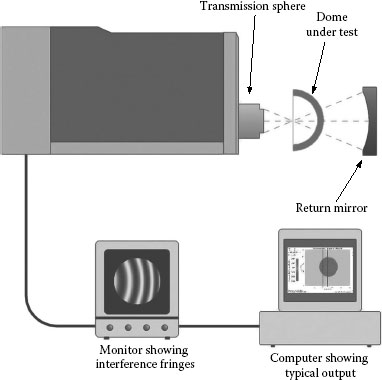
FIGURE 6.25 Testing of domes.
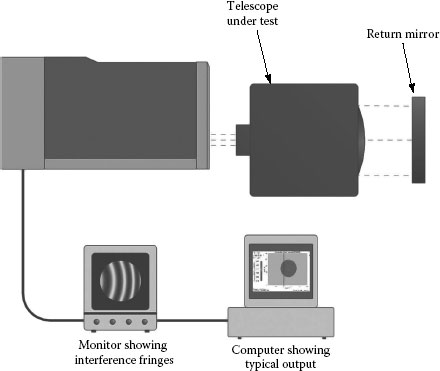
FIGURE 6.26 Testing of telescopes.
Once an interferogram has been obtained it is necessary to analyze it. This can take several forms, the simplest being with a straight edge on a photograph, the most complex being computer-aided fringe analysis. It is not the intent here to describe in detail the fringe analysis software but simply to describe their main points and their availability. Assessing wavefront error from a photograph can be performed as shown in Figure 6.27. This is a relatively crude analysis but is adequate enough for a many applications, though, of course, information from only one fringe is calculated.
Figure 6.28 demonstrates the operation of a simple static fringe digitization software package. Such packages are readily available and are quite adequate for most tasks. However, there are some limitations. The number of digitized points is quite low being typically of the order of 200–300 points.
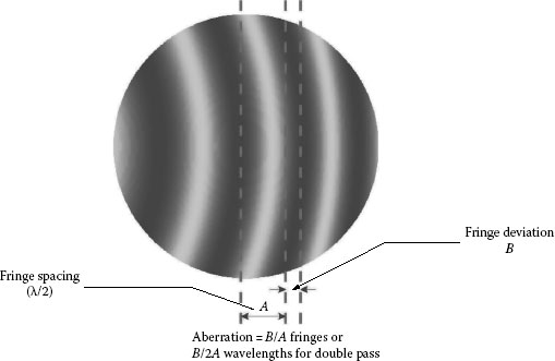
FIGURE 6.27 Simple fringe analysis.
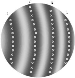
FIGURE 6.28 Digitization of fringe centers.
Additionally there are areas of the optical pupil where there are no digitized points. The software will interpolate for points within the pupil but must extrapolate at the edge of the pupil. The extrapolation can be performed in a number of ways.
• A Zernike polynomial fit is made to the obtained data points, which then provide the wavefront shape. The polynomial coefficients can be used for the extrapolation, but this has the danger that the high-order polynomial could roll off rapidly giving a pessimistic result.
• A linear extrapolation can be performed; this however could ignore any roll off and could provide an optimistic result.
In both the cases mentioned above, it would be unwise to give too much credence to a peak-to-valley wavefront value since it could be out by a large amount. Such figures can still be quoted as results but a hard copy of the interferogram should always be provided. A much more reliable parameter is the root mean square (RMS) wavefront deviation. Normally, information is available over the majority of the optical pupil, therefore effect of roll off due to the polynomial fitting will not have such a large effect. This is fortuitous in that many of the parameters that may be required, particularly for complete optical systems, are based on the RMS wavefront aberration, in particular the Strehl ratio and the MTF. Once the shape of the wavefront is known, then it possible to calculate all geometrical properties of an optical system, MTF, point spread function, encircled energy function, etc.
An important limitation of the above process is that although the fringe shape is known, the sense of that shape is not. That is, we do not know whether a fringe perturbation is a wavefront retardation or advance. This problem is solved, together with the fringe extrapolation problem by using phase-scanning software. This method captures the fringe data over the whole of the optical pupil and by changing phase several times and analyzing the resulting data can determine the initial phase of any pupil point. This provides much greater accuracy particularly where peak-to-valley wavefront deviation is important. A further advantage is that the measurement of material refractive index inhomogeneity can be reliably measured as all other parameters (surface aberrations, etc.) can be measured to high accuracy.
The following curves (Figures 6.29 and 6.30) show that the phase-shifting technique is by far the more accurate. Each curve represents 100 measurements. The two software packages were provided by the same supplier and used the same hardware, for example, computer, interferometer, frame grabber, etc., although the actual component measured was different.
The spread of results with the phase-shifting system is much smaller than with the static system. The static system varies considerably with time as the environment changes. The phase-shifting system was not so badly affected mainly because of the ability to make several measurements and display an average. This has the tendency to smooth out time-dependent variation such as air turbulence, which may be frozen into a static fringe acquisition. It may be expected that the phase-shifting system may suffer more from vibration effects since the measurement process takes longer—the static system simply grabs one frame and thereby freezes the fringe. However, if the fringes are “fluffed out” the software can cope with small vibrations, if the fringes are not fluffed out then more serious effects can occur as they move about.
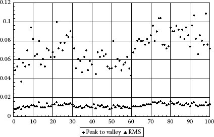
FIGURE 6.29 Variation of measurement with static fringe analysis software.
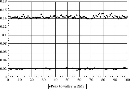
FIGURE 6.30 Variation of measurement with phase-shifting software.
Figure 6.31 shows the fringe patterns obtained for spherical aberration. The pattern on the left is closest to the paraxial focus of the lens under test. The best focus is represented by the central fringe pattern which is also shown three dimensional. This is the position at which the peak-to-valley wavefront error is minimized.
The three positions can be seen again but with tilt fringes added in Figure 6.32.
The wavefront of coma is shown in Figure 6.33. The best focus is the symmetrical pattern shown in the center. Figure 6.34 shows the coma with tilt fringes, again the symmetry of the best focus position is evident.
The familiar saddle shape of astigmatism is shown in Figure 6.35. Again the best focus position is shown at the center. At this point, referenced from the center of the interferogram, the aberration is the same in the horizontal and vertical directions but in opposite directions. Figure 6.36 shows the same situation but with tilt fringes.
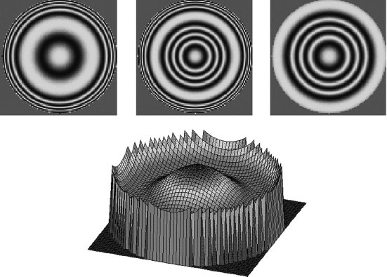
FIGURE 6.31 Spherical aberration.
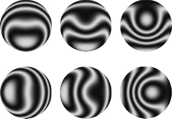
FIGURE 6.32 Spherical aberration with tilt fringes.
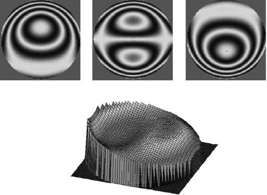
FIGURE 6.33 Coma through focus.
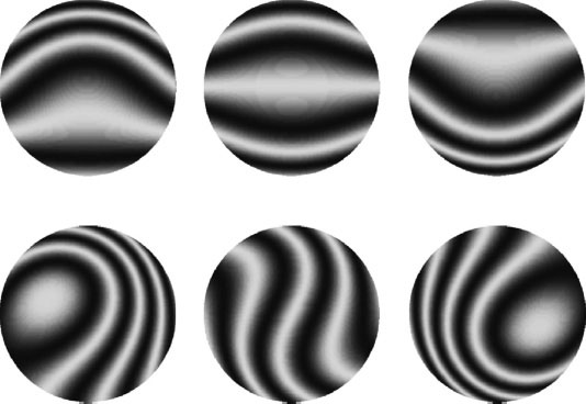
FIGURE 6.34 Coma with tilt fringes.
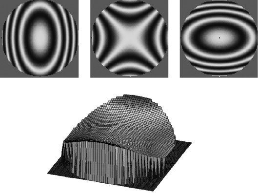
FIGURE 6.35 Astigmatism through focus.
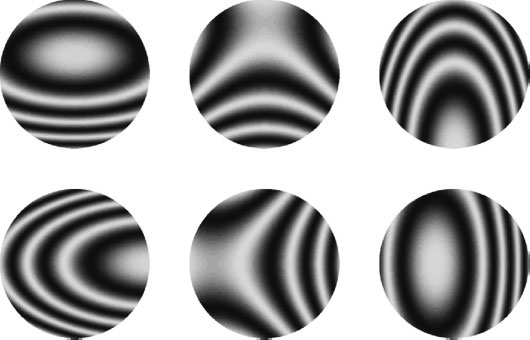
FIGURE 6.36 Astigmatism with tilt fringes.