Chapter 7 Holography

Holography is an interferometric technique that has proved to be convenient to store and reconstruct the complete amplitude and phase information of a wavefront. The popular interest in this technique is due to its unique property to obtain 3D images of an object, but there are other less known but very useful applications that are concerned with microscopy, deformation measurement, aberration correction, beam shaping, optical testing, and data storage, just to mention a few. Since the technique was invented by Gabor [1], as an attempt to increase the resolution in electron microscopy, an extensive research has been done to overcome the original limitations and to develop many of its applications. Gabor demonstrated that if a suitable coherent reference wave is present simultaneously with the light scattered from an object, the information about both the amplitude and the phase of the object wave could be recorded, although the recording media registers only the light intensity. He called this “holography,” from the Greek word holos (the whole), because it contained the whole information. The first concept of holography developed in 1948 was as in-line arrangement using a mercury arc lamp as the light source; it allowed to record only holograms of transparent objects and contained an extraneous twin image. For the next 10 years, holographic techniques and applications did not develop further until the invention of the laser in 1960, whose coherent light was ideal for making holograms. By using a laser source, in 1962, Leith and Upatnieks developed the off-axis reference beam method, which is most often used today [2]. It permitted the making of holograms of solid objects by reflected light.

There are several books describing the principles of holography and their applications; in particular, classical references [3,4,5,6,7,8,9] written in the years from 1969 to 1974 are interesting because together with a clear description of the technique, they predict some developments. In Refs. [6,8], possible commercial applications in the 3D television and information storage are reported. Forty years later, we are still quite far from the holographic television since the electro-optical modulators, for example, liquid crystal displays do not have the necessary spatial resolution, but investigation to circumvent this limitation is in progress. The holographic storage predicted by Lehmann [6] is still not commercially available, but new materials fulfilling the requirements for this application are under development.

In 1966, Brown and Lohmann had described a method for generating holograms by computer and reconstructing images optically [10]; the emerging digital technology had made it possible to create holograms by numerical simulations and print the calculated microstructure on a plate that when illuminated forms a wavefront of a 3D object that does not possess physical reality. This technique is now called computer-generated holography and has useful applications, for example, for correcting aberrations or producing a shaped beam.

The first holograms were recorded on photographic emulsions; these materials have an excellent spatial resolution (typically 2000 lp/mm) and are still used in particular for large-size recording; other high-resolution recording materials are photorefractive crystals and thermoplastic films. Already, in 1967, Goodman [11] has shown that holograms may be recorded on optoelectronic devices, and the physical reconstruction may be replaced by a numerical reconstruction using a computer. This technique, which is now called digital holography, had an impressive development in the last years due in particular to the availability of CCD or CMOS sensors with an increased number of pixels and computer resources. Different arrangements based on digital holography are actually used for applications like microscopic investigations of biological samples, deformation measurement, vibration analysis, and particle visualization.

In this chapter, we will at first review some general concepts about holography; later, the recording of holograms on an electronic device and the digital reconstruction by using a computer are discussed. Some arrangements and their applications for the investigation of microscopic samples, shape contouring, and measurement of deformations will be presented.

7.2 BASIC ARRANGEMENT FOR RECORDING AND RECONSTRUCTING HOLOGRAMS

Basically in holography, two coherent wavefronts, a reference and an object wave, are recorded as an interference pattern (Figure 7.1). We represent the light wavefronts by using scalar functions (scalar wave theory) and consider only purely monochromatic waves; this approximation is sufficient for describing the principle of holography. Let |U_o|, |U_R|, ϕ_o, ϕ_R be the amplitudes and phases of the object and the reference waves, respectively. In Figure 7.1, we use a plane wave to represent the reference, but in the general case, a spherical or any other nonuniform wave may be used for recording the hologram. The complex amplitude of reference and object waves may be written in the exponential form as follows:

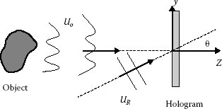
FIGURE 7.1 Hologram recording.

$U_{R} (x, y, z, t) = | U_{R} (x, y, z) | \exp {- i ϕ_{R} (x, y, z)} \exp {i 2 π ν t},$ $U_{R} (x, y, z, t) = | U_{R} (x, y, z) | \exp {- i ϕ_{R} (x, y, z)} \exp {i 2 π ν t},$

(7.1a)

$U_{o} (x, y, z, t) = | U_{o} (x, y, z) | \exp {- i ϕ_{o} (x, y, z)} \exp {i 2 π ν t} .$ $U_{o} (x, y, z, t) = | U_{o} (x, y, z) | \exp {- i ϕ_{o} (x, y, z)} \exp {i 2 π ν t} .$

(7.1b)

In these equations, exp{i2πνt} is a time-varying function, where ν is the frequency, which for visible light has a value in the range 3.8 × 10¹⁴ to 7.7 × 10¹⁴ Hz. The time dependence can be omitted in the description of the holographic process, and the interference between U_o and U_R takes the form

$U_{o R} (x, y, z) = U_{o} (x, y, z) + U_{R} (x, y, z) .$ $U_{o R} (x, y, z) = U_{o} (x, y, z) + U_{R} (x, y, z) .$

(7.2)

The intensity recorded by a detector is given by

$I = (U_{R} + U_{o}) (U_{R}^{*} + U_{o}^{*}) = U_{R} U_{R}^{*} + U_{o} U_{o}^{*} + U_{R}^{*} U_{o} + U_{R} U_{o}^{*},$ $I = (U_{R} + U_{o}) (U_{R}^{*} + U_{o}^{*}) = U_{R} U_{R}^{*} + U_{o} U_{o}^{*} + U_{R}^{*} U_{o} + U_{R} U_{o}^{*},$

(7.3)

where “*” denotes a complex conjugation. Here and what follows to simplify the notation, we have omitted the dependence on (x, y, z). ${| U_{o} |}^{2} = U_{o} U_{o}^{*}$ ${| U_{o} |}^{2} = U_{o} U_{o}^{*}$ and ${| U_{R} |}^{2} = U_{R} U_{R}^{*}$ ${| U_{R} |}^{2} = U_{R} U_{R}^{*}$ are the intensities of the two wavefronts and do not contain any information about the phases; on the other side, we may write the two last terms in the equation as

$\begin{array}{l} U_{R}^{*} U_{o} + U_{R} U_{o}^{*} & = | U_{R} | | U_{o} | [\exp {- i ϕ_{R}} \exp {i ϕ_{0}} + \exp {i ϕ_{R}} \exp {- i ϕ_{0}}] \\ = 2 | U_{R} | | U_{o} | \cos (ϕ_{R} - ϕ_{0}) . \end{array}$ $\begin{array}{l} U_{R}^{*} U_{o} + U_{R} U_{o}^{*} & = | U_{R} | | U_{o} | [\exp {- i ϕ_{R}} \exp {i ϕ_{0}} + \exp {i ϕ_{R}} \exp {- i ϕ_{0}}] \\ = 2 | U_{R} | | U_{o} | \cos (ϕ_{R} - ϕ_{0}) . \end{array}$

(7.4)

Their sum depends on the relative phase, thus the recorded intensity contains information about amplitude and phase of reference and object beams, which is encoded in the interference pattern in the form of a fringe modulation. We may assume that this intensity is recorded on a photosensitive material, for example, a film that was the first used holographic support. After development, we obtain a transparency (we call it hologram) with transmittance proportional to the recorded light intensity. By illuminating the hologram by using the reference wave U_R, we obtain the transmitted wave field

$U_{R} I = U_{R} {| U_{R} |}^{2} + U_{R} {| U_{o} |}^{2} + U_{R} U_{R}^{*} U_{o} + U_{R} U_{R} U_{o}^{*} .$ $U_{R} I = U_{R} {| U_{R} |}^{2} + U_{R} {| U_{o} |}^{2} + U_{R} U_{R}^{*} U_{o} + U_{R} U_{R} U_{o}^{*} .$

(7.5)

The first term U_R|U_R|² represents the reference wave attenuated by the factor |U_R|²; in the second term U_R|U_o|², the reference is modulated by the intensity of the object beam; the third term is nothing else as the object wavefront modulated by the intensity of the reference beam (in principle, we may choose a constant-intensity reference). Since the reconstruction of the third term has exactly the same properties as the original wave, an observer perceives it as coming from a virtual image of the object located exactly at the original object location (see Figure 7.2). The last term contains the complex conjugate of the object beam $U_{o}^{*}$ $U_{o}^{*}$ ; the best way for reconstructing this field is to illuminate the hologram with a conjugate of the reference wave $U_{R}^{*}$ $U_{R}^{*}$ , as shown in Figure 7.3. In the in-line arrangement proposed by Gabor [1], the four reconstructions were superimposed; in the off-axis configuration illustrated in Figures 7.1 through 7.3, the angle θ between reference and object wave allows an easy spatial separation of the waves.

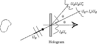
FIGURE 7.2 Reconstruction of the virtual image of the subject.

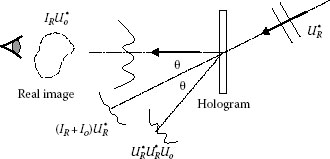
FIGURE 7.3 Reconstruction of the real image of the subject.

The holographic process is not limited to visible light; thus, in principle, hologram may be recorded by using UV and X-rays for which frequency is higher (10¹⁵–10¹⁸ Hz) compared to the visible radiation.

7.3 FOURIER ANALYSIS OF THE HOLOGRAM

The Fourier transform (FT) is one of the most important mathematical tools and is frequently used to describe several optical phenomena like wave propagation, filtering, image formation, and the analysis of holograms. We will see later how it can be used for the digital reconstruction of holographic wave fields. The formulas relating a 2D function f(x, y) and its FT $\tilde{f} (f_{x}, f_{y})$ $\tilde{f} (f_{x}, f_{y})$ are the following:

$\tilde{f} (f_{x}, f_{y}) = \int_{- \infty}^{\infty} \int_{- \infty}^{\infty} f (x, y) \exp {2 π i (x f_{x} + y f_{y})} d x d y,$ $\tilde{f} (f_{x}, f_{y}) = \int_{- \infty}^{\infty} \int_{- \infty}^{\infty} f (x, y) \exp {2 π i (x f_{x} + y f_{y})} d x d y,$

(7.6a)

$f (x, y) = \int_{- \infty}^{\infty} \int_{- \infty}^{\infty} \tilde{f} (f_{x}, f_{y}) \exp {- 2 π i (x f_{x} + y f_{y})} d f_{x} d f_{y} .$ $f (x, y) = \int_{- \infty}^{\infty} \int_{- \infty}^{\infty} \tilde{f} (f_{x}, f_{y}) \exp {- 2 π i (x f_{x} + y f_{y})} d f_{x} d f_{y} .$

(7.6b)

Sometimes, we will use the notations $\tilde{f} (f_{x}, f_{y}) = F T {f (x, y)}$ $\tilde{f} (f_{x}, f_{y}) = F T {f (x, y)}$ and $f (x, y) = F T^{- 1} {\tilde{f} (f_{x}, f_{y})}$ $f (x, y) = F T^{- 1} {\tilde{f} (f_{x}, f_{y})}$ , where FT and FT⁻¹ are the FT and its inverse, respectively. The convolution (denoted by the symbol ⊗) between two functions f(x, y) and g(x, y)

$h (x^{'}, y^{'}) = f \otimes g = \int_{- \infty}^{\infty} \int_{- \infty}^{\infty} f (x, y) g (x^{'} - x, y^{'} - y) d x d y$ $h (x^{'}, y^{'}) = f \otimes g = \int_{- \infty}^{\infty} \int_{- \infty}^{\infty} f (x, y) g (x^{'} - x, y^{'} - y) d x d y$

(7.7)

is another important mathematical tool that we need for our analysis.

The Fourier transform of the holographically reconstructed wavefront is equal to the sum of the FT of four individual terms:

$F T {U_{R} I} = F T {U_{R} {| U_{R} |}^{2}} + F T {U_{R} {| U_{o} |}^{2}} + F T {U_{R} U_{R}^{*} U_{o}} + F T {U_{R} U_{R} U_{o}^{*}} .$ $F T {U_{R} I} = F T {U_{R} {| U_{R} |}^{2}} + F T {U_{R} {| U_{o} |}^{2}} + F T {U_{R} U_{R}^{*} U_{o}} + F T {U_{R} U_{R} U_{o}^{*}} .$

(7.8)

We consider a hologram recorded by using a plane reference wave having constant amplitude |U_R| propagating in the direction (0, sin θ, cos θ)

$U_{R} (x, y, z) = | U_{R} (x, y, z) | \exp {2 π i [y \sin θ + z cos θ] / λ},$ $U_{R} (x, y, z) = | U_{R} (x, y, z) | \exp {2 π i [y \sin θ + z cos θ] / λ},$

(7.9)

where λ is the laser wavelength; in writing the waves, we shall normally omit the propagation constant for the z direction. The spectrum of the hologram distribution (absolute value of the FT of the reconstructed wavefront) is schematically shown in Figure 7.4a. Since the reference is a plane wave, the FT of U_R |U_R|² is a delta function δ(f_x, f_y − f_r), centered at f_x = 0, f_y = f_r, where f_x, f_y are the spatial frequencies and f_r = sin θ/λ; in the frequency domain, this term will be concentrated on a single point. By using the convolution theorem, which states that a multiplication in the spatial domain equals convolution in the spatial-frequency domain, we obtain for the second term the relation

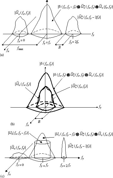
FIGURE 7.4 Spectrums of holograms. Off-axis (a) and in-line (b). Asymmetrical spectrums of an off-axis hologram (c).

$F T {U_{R} (x, y) U_{o}^{*} (x, y) U_{o} (x, y)} = {\tilde{U}}_{R} (f_{x}, f_{y}) \otimes {\tilde{U}}_{o}^{*} (f_{x}, f_{y}) \otimes {\tilde{U}}_{o} (f_{x}, f_{y}) .$ $F T {U_{R} (x, y) U_{o}^{*} (x, y) U_{o} (x, y)} = {\tilde{U}}_{R} (f_{x}, f_{y}) \otimes {\tilde{U}}_{o}^{*} (f_{x}, f_{y}) \otimes {\tilde{U}}_{o} (f_{x}, f_{y}) .$

(7.10)

If the object has frequency components not higher than B, then the convolution term expressed by Equation 7.10 has an extension equal to 2B and like the first term is centered at f_x = 0, f_y = f_r.

The third and the fourth terms in Equation 7.8 are given by

$F T {U_{R} (x, y) U_{R}^{*} (x, y) U_{o} (x, y)} = {\tilde{U}}_{R} (f_{x}, f_{y}) \otimes {\tilde{U}}_{R}^{*} (f_{x}, f_{y}) \otimes {\tilde{U}}_{o} (f_{x}, f_{y}) = {\tilde{U}}_{o} (f_{x}, f_{y}),$ $F T {U_{R} (x, y) U_{R}^{*} (x, y) U_{o} (x, y)} = {\tilde{U}}_{R} (f_{x}, f_{y}) \otimes {\tilde{U}}_{R}^{*} (f_{x}, f_{y}) \otimes {\tilde{U}}_{o} (f_{x}, f_{y}) = {\tilde{U}}_{o} (f_{x}, f_{y}),$

(7.11a)

$\begin{array}{l} F T {U_{R} (x, y) U_{R} (x, y) U_{o}^{*} (x, y)} & = {\tilde{U}}_{R} (f_{x}, f_{y}) \otimes {\tilde{U}}_{R} (f_{x}, f_{y}) \otimes {\tilde{U}}_{o}^{*} (f_{x}, f_{y}) \\ = δ (f_{x}, f_{y} - 2 f_{r}) \otimes {\tilde{U}}_{o}^{*} (f_{x}, f_{y}) . \end{array}$ $\begin{array}{l} F T {U_{R} (x, y) U_{R} (x, y) U_{o}^{*} (x, y)} & = {\tilde{U}}_{R} (f_{x}, f_{y}) \otimes {\tilde{U}}_{R} (f_{x}, f_{y}) \otimes {\tilde{U}}_{o}^{*} (f_{x}, f_{y}) \\ = δ (f_{x}, f_{y} - 2 f_{r}) \otimes {\tilde{U}}_{o}^{*} (f_{x}, f_{y}) . \end{array}$

(7.11b)

These relations were obtained by considering that ${\tilde{U}}_{R} (f_{x}, f_{y}) = δ (f_{x}, f_{y} - f_{r})$ ${\tilde{U}}_{R} (f_{x}, f_{y}) = δ (f_{x}, f_{y} - f_{r})$ and ${\tilde{U}}_{R}^{*} (f_{x}, f_{y}) = δ (f_{x}, f_{y} + f_{r})$ ${\tilde{U}}_{R}^{*} (f_{x}, f_{y}) = δ (f_{x}, f_{y} + f_{r})$ , respectively. In order to obtain a spatial separation of the object reconstructions terms from the self-interference term, it is necessary that f_r ≥ 3B.

The maximal angle between the reference and the object wave θ_max determines the maximal spatial frequency f_max in the hologram:

$f_{\max} = \frac{2}{λ} \sin [\frac{θ_{max}}{2}] .$ $f_{\max} = \frac{2}{λ} \sin [\frac{θ_{max}}{2}] .$

(7.12)

The resolution of the recording device should be able to record this spatial frequency in order to obtain a spatial separation of the reconstructed waves. Figure 7.4b illustrates the spectrum of an in-line Gabor hologram recorded by using a reference plane wave propagating in the same direction as the object field; thus, in Equation 7.9, the angle θ is equal to 0 and ${\tilde{U}}_{R} (f_{x}, f_{y}) = {\tilde{U}}_{R}^{*} (f_{x}, f_{y}) = δ (f_{x}, f_{y})$ ${\tilde{U}}_{R} (f_{x}, f_{y}) = {\tilde{U}}_{R}^{*} (f_{x}, f_{y}) = δ (f_{x}, f_{y})$ . The four terms are overlapped; we will see later that by using digital holography together with a phase-shifting technique, it is possible to separate these terms. Until now, we considered a plane reference wave because this makes the mathematical treatment easier; if we use another reference (e.g., a spherical wave), we will obtain asymmetrical spectra like that shown in Figure 7.4c. The spectra in Figure 7.4 describe the separation of the terms far away from the hologram (Fraunhofer diffraction or equivalently far field); at a shorter distance, the light distributions will be different, but if the reconstructions are separated at the infinity, it is usually possible to obtain their separation at a shorter distance.

7.4 DIGITAL HOLOGRAPHY

7.4.1 HISTORICAL REMARKS AND TECHNOLOGICAL DEVELOPMENTS

In classical holography, the interferences between reference and object waves are stored on high-resolution photographic emulsions, occasionally on photo-thermo plastic or photorefractive material. For the reconstruction, a coherent wave, usually a laser, is used. The process is time consuming, particularly with respect to the development of the photographic film.

In 1967, Goodman and Lawrence [11] reported the first case of detection of a hologram by means of an electro-optical device; they used a vidicon to sample the hologram on a 256 × 256 array, and the digital reconstruction was done by using a PDP-6 computer. For this kind of reconstruction, fast Fourier transform (FFT) algorithms have been used. In a conference paper [12], Goodman explained that this experiment was motivated by the desire to form images of actively illuminated satellites free from the disturbing effects produced by the earth atmosphere. Interesting is to notice that a 256 × 256 FFT transform took about 5 min in 1967 by using one of the most powerful computers available at that time; now (2014) a typical personal computer performs this computation in only few milliseconds.

The procedures for digitally reconstructing holograms were further developed in the seventies years in particular by Yaroslavskii and others [13,14]. They digitized one part of a conventional hologram recorded on a photographic plate and fed those data to a computer; the digital reconstruction was obtained by a numerical implementation of the diffraction integral.

During the last 30 years, we had an impressive development of the charge-coupled devices (CCDs) that were invented in 1969 but became commercially available only since 1980. Complementary metal–oxide–semiconductor sensors (CMOS) are another type of electro-optical sensors having almost the same sensitivity and signal-to-noise ratio as the CCDs. Both CCD and CMOS can have several thousands of pixels in each direction (e.g., 4000 × 4000), a typical pixel size of 5 × 5 μm² and a dynamic range of 8–10 bits, which may be increased to 12–14 bits by using a cooling system. Those devices have become an attractive alternative to photographic film, photo–thermoplastic, and photorefractive crystals as recording media in holography. The time-consuming wet processing of photographic film is avoided, and the physical reconstruction of holograms can be replaced by a numerical reconstruction using a computer, normally an ordinary PC. Haddad et al. [15] were probably the first to report the recording of a hologram on a CCD. They used a lensless arrangement for the recording of a wavefront transmitted by a microscopic biological sample and were able to obtain reconstructions with a resolution of 1 μm. During the past 20 years, several arrangements have been developed for the investigation of transmission and reflection of both technical and biological samples. Digital holographic microscopy [15,16,17,18,19,20,21,22,23,24,25,26,27,28,29,30,31,32,33,34,35,36,37,38,39,40] allows high-resolution 3D representations of microstructures and provides quantitative phase contrast images. Recording of digital holograms of macroscopic objects is reported in Refs. [41,42,43,44,45,46]; most of these published works combine the holographic technique with interferometry in order to measure deformations of mechanical components and biological tissues. Excellent books describing the methods of digital holography and digital holographic interferometry are available [47,48,49,50].

7.4.2 LIMITATIONS DUE TO THE RECORDING OF HOLOGRAMS ON AN ELECTRO-OPTICAL DEVICE

One disadvantage, however, of using electro-optical sensors for hologram recording is the relatively low spatial resolution, compared to that of photographic material or photorefractive crystals. The recording of holograms on low-resolution media has been discussed in many books and publications [4–9,47–50]. The spatial resolution of commercially available CCD and CMOS is typically 200 lines/mm, which is much poorer than photographic films (5000 lines/mm); this limits the spatial frequency that can be recorded using these devices. To record a hologram of the entire object, the resolution must be sufficient to resolve the fringes formed by the reference wave and the wave coming from any object point. Consider that the intensity described by Equation 7.3 is recorded on a 2D array of sensors (M × N cells) of dimension Δx × Δy. For the most common case of equidistant cells, we have Δx = Δy =Δ, and the discrete recorded intensity can be written in the form I(mΔ, nΔ), where n and m are integer numbers. From the sampling theorem (see, e.g., Ref. [50]), it is necessary to have at least two sampled points for each fringe; therefore, the maximum spatial frequency that can be recorded is

$f_{\max} = 1 \frac{2}{Δ} .$ $f_{\max} = 1 \frac{2}{Δ} .$

(7.13)

By inserting this in Equation 7.12, we obtain the condition for θ_max: sin(θ_max/2) ≤ λ/(4Δ) and for small angles θ_max ≤ λ/(2Δ).

7.4.3 MATHEMATICAL TOOLS FOR THE DIGITAL RECONSTRUCTION OF A HOLOGRAM

From the diffraction theory, we know that if the amplitude and phase of a wavefront are known at a plane (x₁, y₁), it is possible to calculate the propagation of such wavefront in the plane (x₂, y₂) (see Figure 7.5). For calculating the diffracted wavefront, there are different approximations. If we consider the Rayleigh–Sommerfeld diffraction integral (see, e.g., Ref. [51]), the wave fields at the plane (x₂, y₂) located at a distance d from the plane (x₁, y₁) are given by

$U_{2} (x_{2}, y_{2}) = \frac{i}{λ} \iint U_{1} (x_{1}, y_{1}) \frac{e^{i k η_{2}}}{r_{12}} \cos α d x_{1} d y_{1},$ $U_{2} (x_{2}, y_{2}) = \frac{i}{λ} \iint U_{1} (x_{1}, y_{1}) \frac{e^{i k η_{2}}}{r_{12}} \cos α d x_{1} d y_{1},$

(7.14)

where

$r_{12} = \sqrt{d^{2} + {(x_{2} - x_{1})}^{2} + {(y_{2} - y_{1})}^{2}}$ $r_{12} = \sqrt{d^{2} + {(x_{2} - x_{1})}^{2} + {(y_{2} - y_{1})}^{2}}$

k = 2π/λ

cos α is the obliquity factor

In the following, the obliquity factor will be neglected. The diffraction integral can be written as a convolution

$U_{2} (x_{2}, y_{2}) = \frac{i}{λ} \iint U_{1} (x_{1}, y_{1}) g (x_{2} - x_{1}, y_{2} - y_{1}) d x_{1} d y_{1} = U_{1} \otimes g,$ $U_{2} (x_{2}, y_{2}) = \frac{i}{λ} \iint U_{1} (x_{1}, y_{1}) g (x_{2} - x_{1}, y_{2} - y_{1}) d x_{1} d y_{1} = U_{1} \otimes g,$

(7.15)

where

$g (x_{2} - x_{1}, y_{2} - y_{1}) = \frac{i \exp {i k \sqrt{d^{2} + {(x_{2} - x_{1})}^{2} + {(y_{2} - y_{1})}^{2}}}}{λ \sqrt{d^{2} + {(x_{2} - x_{1})}^{2} + {(y_{2} - y_{1})}^{2}}}$ $g (x_{2} - x_{1}, y_{2} - y_{1}) = \frac{i \exp {i k \sqrt{d^{2} + {(x_{2} - x_{1})}^{2} + {(y_{2} - y_{1})}^{2}}}}{λ \sqrt{d^{2} + {(x_{2} - x_{1})}^{2} + {(y_{2} - y_{1})}^{2}}}$

(7.16)

is the impulse response of the free-space propagation. According to the Fourier theory, the convolution integral between two functions may be calculated by multiplying their individual FTs followed by an inverse FT, and thus, Equation 7.15 may be rewritten in the form

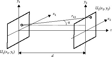
$U_{2} (x_{2}, y_{2}) = F T^{- 1} {F T {U_{1} (x_{1}, y_{1})} F T {g (x_{1}, y_{1})}} .$ $U_{2} (x_{2}, y_{2}) = F T^{- 1} {F T {U_{1} (x_{1}, y_{1})} F T {g (x_{1}, y_{1})}} .$

(7.17)

FIGURE 7.5 Diffraction geometry.

If the distance d is large compared with (x₁ − x₂) and (y₁ − y₂), the binominal expansion of the square root up to the third term yields

$r_{12} \approx d [1 + \frac{{(x_{1} - x_{2})}^{2}}{2 d} + \frac{{(y_{1} - y_{2})}^{2}}{2 d}] .$ $r_{12} \approx d [1 + \frac{{(x_{1} - x_{2})}^{2}}{2 d} + \frac{{(y_{1} - y_{2})}^{2}}{2 d}] .$

(7.18)

By inserting Equation 7.18 in Equation 7.15, we obtain the Fresnel approximation of the diffraction integral:

$U_{2} (x_{2}, y_{2}) = \frac{e^{i k d} e^{i k \frac{(x_{2}^{2} + y_{2}^{2})}{2 d}}}{i λ d} \iint U_{1} (x_{1}, y_{1}) e^{i k \frac{(x_{1}^{2} + y_{1}^{2})}{2 d}} e^{- i k \frac{(x_{1} x_{2} + y_{1} y_{2})}{d}} d x_{1} d y_{1} .$ $U_{2} (x_{2}, y_{2}) = \frac{e^{i k d} e^{i k \frac{(x_{2}^{2} + y_{2}^{2})}{2 d}}}{i λ d} \iint U_{1} (x_{1}, y_{1}) e^{i k \frac{(x_{1}^{2} + y_{1}^{2})}{2 d}} e^{- i k \frac{(x_{1} x_{2} + y_{1} y_{2})}{d}} d x_{1} d y_{1} .$

(7.19)

This can be seen as a FT of $U (x_{1}, y_{1}) \exp {i k [x_{1}^{2} + y_{1}^{2}] / (2 d)}$ $U (x_{1}, y_{1}) \exp {i k [x_{1}^{2} + y_{1}^{2}] / (2 d)}$ multiplied by a quadratic factor.

In digital holography, the intensity is recorded on a discrete array of sensors I(mΔx, nΔy), and for the digital calculation of the propagation, it is necessary to use a discrete form of Equations 7.14 through 7.19. If we consider a digitized wave field (e.g., formed by M × N = 1000 × 1000 points), it would take a very long time to compute the convolution between the two functions U₁ and exp{ikr₁₂}/r₁₂ described by Equation 7.14; the direct use of such equation is thus not recommended. A more suitable way for the wavefront calculation is to use the 2D discrete FTs. The discrete forms of Equation 7.6 are

$\tilde{f} (r, s) = \sum_{m = 0}^{M - 1} \sum_{n = 0}^{N - 1} f (m, n) \exp {2 π i [\frac{m r}{M} + \frac{n s}{N}]},$ $\tilde{f} (r, s) = \sum_{m = 0}^{M - 1} \sum_{n = 0}^{N - 1} f (m, n) \exp {2 π i [\frac{m r}{M} + \frac{n s}{N}]},$

(7.20a)

$f (m, n) = \sum_{r = 0}^{M - 1} \sum_{s = 0}^{N - 1} \tilde{f} (r, s) \exp {- 2 π i [\frac{m r}{M} + \frac{n s}{N}]},$ $f (m, n) = \sum_{r = 0}^{M - 1} \sum_{s = 0}^{N - 1} \tilde{f} (r, s) \exp {- 2 π i [\frac{m r}{M} + \frac{n s}{N}]},$

(7.20b)

where r, s, m, n are integer numbers. Fortunately, the 2D discrete FT can be calculated in a short time by using the FFT algorithm (some milliseconds for M × N = 1000 × 1000) allowing the fast computation of the wavefront propagation. A rigorous mathematical description of the reconstruction of discrete wavefronts by using FFT transforms may be found in Refs. [14, 47–50]; here, we just give the discrete form of Equation 7.19 representing the Fresnel propagation from a plane (x₁, y₁), where the input is discretized on M × N array of pixels having size (Δx₁, Δy₁), to an M × N array of pixels having size (Δx₂, Δy₂) in the plane (x₂, y₂):

$U_{2} (r Δ x_{2}, s Δ y_{2}) = e^{i k d} e^{\frac{i π}{d λ} {Δ x_{2}^{2} r^{2} + Δ y_{2}^{2} s^{2}}} \sum_{m = 0}^{M - 1} \sum_{n = 0}^{N - 1} U_{1} (m Δ x_{1}, n Δ y_{1}) e^{\frac{i π}{d λ} {m^{2} Δ x_{1}^{2} + n^{2} Δ y_{1}^{2}}} e^{- 2 π {\frac{m r}{M} + \frac{n s}{N}}}$ $U_{2} (r Δ x_{2}, s Δ y_{2}) = e^{i k d} e^{\frac{i π}{d λ} {Δ x_{2}^{2} r^{2} + Δ y_{2}^{2} s^{2}}} \sum_{m = 0}^{M - 1} \sum_{n = 0}^{N - 1} U_{1} (m Δ x_{1}, n Δ y_{1}) e^{\frac{i π}{d λ} {m^{2} Δ x_{1}^{2} + n^{2} Δ y_{1}^{2}}} e^{- 2 π {\frac{m r}{M} + \frac{n s}{N}}}$

(7.21)

The pixel size in the two planes is given by

$Δ x_{2} = \frac{d λ}{M Δ x_{1}}, Δ y_{2} = \frac{d λ}{N Δ y_{1}} .$ $Δ x_{2} = \frac{d λ}{M Δ x_{1}}, Δ y_{2} = \frac{d λ}{N Δ y_{1}} .$

(7.22)

For this special relation, the last exponential term in Equation 7.21 has exactly the form of the last exponent in the discrete FT 7.20, and the Fresnel propagation can be calculated by using a fast algorithm (FFT). The numerical calculation of the propagation according to the discrete form of Equation 7.17 (sometimes this is simply called convolution algorithm [49,50]) employs three FFTs and is thus more time consuming compared with the simple discrete Fresnel transform described by Equation 7.21. By using the convolution algorithm, the pixel spacing is always the same, while in the Fresnel algorithm, it proportionally depends on the product of the wavelength and the reconstruction distance. Two-step Fresnel reconstruction algorithms have been developed (double Fresnel transform algorithm [52]) allowing to adjust the pixel spacing in the reconstructed wavefront.

After this mathematical review of the formula of wave propagation, we may now consider some recording geometries and the corresponding reconstruction method.

7.4.4 SOME ARRANGEMENTS FOR DIGITAL HOLOGRAPHY

Classical and digital holograms may be classified according to the geometry used for the recording. We consider at first a lensless off-axis setup (Figure 7.6a). The only difference between the lensless arrangement used for the recording of a classical and a digital hologram is that for the digital recording, the angle between object and reference should be small in order to allow the low-resolution digital sensor to sample the interference pattern. The recorded intensity I(mΔx, nΔy) is multiplied with a numerical representation of the reference wave followed by numerical calculation of the resulting diffraction field. Usually, plane or spherical uniform waves are used for recording digital holograms, since these waves can be easily simulated during the reconstruction process. Figure 7.6b through d shows three reconstructions of small objects (5 cm); the digital focusing allows, without any mechanical movements, to focalize any plane along the z axis. For recording the hologram, a spherical reference originating from a point source located close to the object has been used. The reconstructions display the characteristic image pair described by $U_{R} U_{R}^{*} U_{o}^{*}$ $U_{R} U_{R}^{*} U_{o}^{*}$ and $U_{R} U_{R} U_{o}^{*}$ $U_{R} U_{R} U_{o}^{*}$ flanking a central bright spot representing the spherical wave U_R |U_R|² focusing at the object plane. The convolution term that according to Figure 7.4a has twice the extension of the object term is spread over the whole field. For recording this hologram, the condition f_r ≥ 3B was not satisfied, but the reference wave was much stronger compared with the object wave; this decreases the magnitude of the convolution term compared with the reconstructed image as shown schematically in Figure 7.6e. For the hologram recording, the distance between the CCD and the object was 100 cm.

If the object is large and the sensor has limited resolution, it is necessary to locate the object far away from the recording device in order to satisfy the sampling theorem. We illustrate this by a simple example where an object having dimension L_o = 1 m is holographically recorded on a CCD having pixel size Δ = 5 μm by using light with a wavelength of 0.5 μm. The maximal allowable angle between reference and object (θ_max ≈ L_o/a) should satisfy the condition θ_max < λ/(2Δ); thus, a should be larger than 2L_oΔ/λ = 20 m. In practice, the lensless arrangement is not suitable for recording digital holograms of large objects by using CCDs or CMOS. This problem can be solved by inserting a lens and an aperture having dimension L_A between the object and the sensor (Figure 7.7a). L_A is usually few millimeters, and the sampling condition is satisfied when the distance b between aperture and sensor is some centimeters.

For recording digital holograms of microscopical samples, the arrangement shown in Figure 7.7b is usually used; in this last case, a microscope objective images the object on the sensor or at any other plane.

For both the arrangements shown in Figure 7.7a and b, the reference is a spherical wave originating from a point located close to the aperture; by performing a FT of the recorded intensity, we obtain two reconstructions (primary and secondary) together with the central convolution term. When these terms are well separated (as in the case of Figure 7.7c), we can select one reconstruction where the information about the amplitude and phase of the wavefront at the plane of the aperture is included (see Figure 7.7d). After filtering, we propagate the wavefront at any other plane to obtain digital focused images.

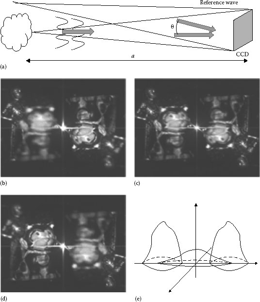
FIGURE 7.6 Lensless arrangement for digital holography (a). Digital reconstructions of small objects at three different planes (b, c, d). Spectra of the hologram (e).

A disadvantage of an off-axis configuration is that the tilted reference, necessary for introducing the carrier fringes and separating the reconstructions, increases the spatial frequencies contained in the hologram, and this prohibits the effective use of all the pixels of the array sensor. This problem can be reduced by using a phase-shifting technique, in which the phase and amplitude information of the object beam are obtained through an in-line setup (see Figure 7.8), with no inclination between object and reference beams [53]. A mirror mounted on a piezoelectric transducer is used to shift stepwise the phase of the reference beam. Several interferograms with mutual phase shift are recorded and used for calculating the phase of the object wave. The disadvantage of the method is that at least three interferograms need to be recorded; this makes it not well suited for investigations of dynamical events, restricting its application to slow-varying phenomena. The in-line arrangement may be modified by inserting a lens in the object wavefront; this can be particularly useful for microscopic investigations.

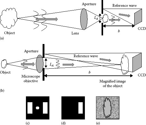
FIGURE 7.7 Arrangement for recording hologram of large (a) and microscopical (b) objects where a lens and an aperture are inserted between object and sensor. Reconstruction of amplitude and phase in the plane of the aperture by FFT of the recorded intensity (c), filtering (d) and image reconstruction by digital propagation of the wavefront (e).

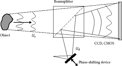
FIGURE 7.8 Arrangement for the recording of a lensless in-line digital hologram.

7.5 APPLICATIONS OF DIGITAL HOLOGRAPHY

Digital holography has been proposed for several applications; in this section, we report few results showing that it can be used for the investigations of microscopical samples, for shape contouring and for the measurement of displacements.

7.5.1 DIGITAL HOLOGRAPHIC MICROSCOPY

Digital holography has been broadly applied to microscopy; some groups use a lensless setup where the sensor records the interference between the light scattered by the object and the reference; others prefer to introduce a lens (e.g., a microscope objective) in order to image the sample to a plane behind the sensor (see Figure 7.7b).

Being a scan-less and also a label-free technique, digital holographic microscopy can be used to extract the 3D information of the organism using a single image (digital hologram). The quantitative phase and amplitude information of the object wavefront can be digitally obtained along the depth of the object from the recorded hologram, which makes it possible to digitally focus on different layers of the specimen and reconstruct a 3D profile of the optical thickness of the organism using the quantitative phase value. Figure 7.9 shows that digital holography can be used for bright- and dark-field reconstructions of amplitude and phases of a sea urchin larva. Because of having no background in dark-field imaging, the noise coming from the coherent light in the background is suppressed, leading to a significant contrast enhancement [38].

Like in conventional microscopy, the spatial resolution of digital holographic microscopy is given by

$δ x = \frac{κ_{1} λ}{N A_{i m a g} + N A_{i l l u m}},$ $δ x = \frac{κ_{1} λ}{N A_{i m a g} + N A_{i l l u m}},$

(7.23)

where

NA_imag and NA_illum are the numerical aperture of the illumination and imaging systems, respectively

λ is the wavelength

κ₁ is the factor determined by experimental parameters, such as coherent noise level, signal-to-noise ratio of the detector [54]

The spatial resolution can thus be improved by using a short wavelength or synthesizing a larger NA, which can be obtained by off-axis illumination or projecting a periodic pattern onto a specimen.

An arrangement that uses a short wavelength is reported in Ref. [40], and thus according to Equation 7.23, the resolution is increased. The light source was an excimer laser emitting radiation at 193 nm; all the optical elements (beamsplitter, lenses, waveplates, and polarizers) were made of fused silica. These materials have a good transmission in the ultraviolet light. A custom-design objective with large numerical aperture NA_imag = 0.75 and 1 mm focal length was used. To further improve the resolution, oblique illumination allowing to increase the numerical aperture NA_illum is implemented in the setup. A digital camera is commercially available for this wavelength with high UV sensitivity, which can perform direct imaging with no filter or fluorescent. Figure 7.10a shows a scanning electron microscope image of the nano-structured template designed to examine the resolution of the holographic system. The template is made of 35 nm of gold layer coated by ion-beam sputtering on a fused silica substrate. It includes square and line structures, ranging from 100 to 500 nm in width. The logo of the Institut für Technische Optik “ito” is also included in the template in which its elements have a width of ~300 nm. The image taken by an optical microscope (Zeiss Axiovert 200, with × 100 objective, NA = 0.7) is shown in Figure 7.10b. The reconstructed amplitude and phase obtained by digital holography are shown in Figure 7.10c and d, respectively. In Figure 7.10c, the “ito” logo is clear, and even the line structures with the width of 250 nm are well resolved.

7.5.2 DIGITAL HOLOGRAPHIC SECTIONING BY USING A SHORT COHERENCE LIGHT SOURCE

Several imaging techniques, such as coherence radar [55] or digital light-in-flight holography [56], take advantage of low temporal coherence to examine 3D objects. Furthermore, optical coherence tomography (OCT) [57] provides high-resolution cross-sectional images of the internal microstructure of materials and biological samples. As has been reported in Refs. [58,59], the use of short coherence digital holography allows optical sectioning and has the ability to discriminate light coming from different planes of a sample. In Ref. [60], the light source was a short coherence laser diode, and a lensless in-line arrangement like that shown in Figure 7.8 has been used. The phase of the wavefront was recovered by using a phase-shifting method. Due to the short coherence of the laser, the interference is just observed when the optical path lengths of reference and object beams are matched within the coherence length of the laser; the numerical reconstruction of the hologram theoretically corresponds to a defined layer, and reconstruction gets rid of any spurious light coming from other parts of the sample. The selection of the plane of interest can be simply performed by mechanical shifting of a mirror in the experimental setup that changes the path difference between object and reference. Some advantages of this method over other imaging techniques allowing optical sectioning, like confocal microscopy or OCT, are the simplicity of the optical arrangement and the possibility to record at once the whole information about the plane of interest, without any need of lateral scanning. In Figure 7.11 are shown the images of different layers of a fly with an interval of 0.1 mm between each image.

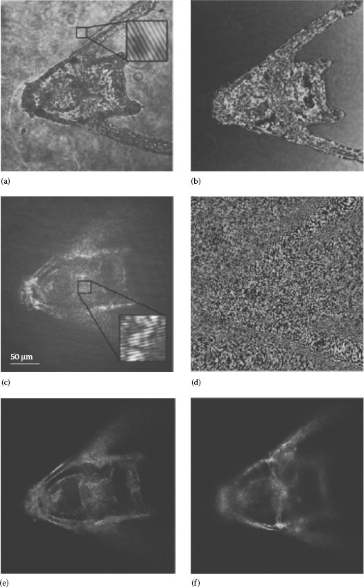
FIGURE 7.9 Bright-field hologram of a sea urchin larva illuminated by a short coherence source (a) and reconstructed phase (b). Dark-field hologram (c), phase (d) and intensity reconstructions at two focus planes (e and f). The holograms are taken by a bright/dark-field objective (20×, NA = 0.45). (From Faridian, A. et al., J. Biomed. Opt., 18(8), 086009, 2013.)

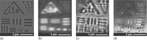
FIGURE 7.10 Scanning electron microscope image of the nano-structured template (a); image taken by a conventional optical microscope with NA = 0.75, × 100 objective (b); the reconstructed amplitude (c) and phase (d) of the object. (From Faridian, A. et al., Opt. Express, 18(13), 14159, 2010.)

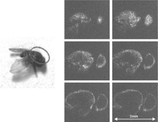
FIGURE 7.11 Reconstructed images of a fly. (From Martínez-León, L. et al., Appl. Opt., 44, 3977, 2005.)

In Ref. [61], it was demonstrated how short temporal coherence digital holography with a femtosecond frequency comb laser source may be used for multilevel optical sectioning. In contrast to conventional approaches, each hologram reconstructs not only the section of the object where reference and object beam matches, but as well other planes with equidistant intervals. Figure 7.12 shows an experimental result, where the object used for the investigation was a metallic cone with half angle of 12°, 80 mm coned length and 36 mm base diameter (see Figure 7.12a). Figure 7.12b through d shows three numerical reconstructions obtained from a single hologram with digital focusing in three different planes, each separated by 25 mm. In Figure 7.12b, we see a ring with small radius at the center that corresponds to the intersection of the cone with a plane (we will call this PL-1); in the same figure, there are two other rings with larger radius describing intersections of the object with two planes (PL-2 and PL-3) axially spaced by 25 and 50 mm with respect to PL-1. Three rings appear because we use a frequency comb laser having a periodical coherence function displaying peaks spatially separated by 50 mm. A conventional short coherence or a femtosecond laser provides single sectioning only. In Figure 7.12b, the intersection lines of the cone with PL-2 and PL-3 are blurred since the reduced depth of focus does not allow to reconstruct sharp profiles located at different planes. Figure 7.12c and d shows that digital focusing of the hologram allows to obtain sharp profile lines at PL-3 and PL-2, respectively. The three reconstructed profiles obtained from a single hologram do not allow to retrieve the complete 3D shape of the object. More sections would be necessary for this purpose, which could be obtained by using an fc-laser having larger frequency comb spacing and thus a reduced axial plane separation. The scanning method was used to obtain more section profiles, where the path length of the reference beam was changed by shifting the reference mirror, and a sequence of holograms was recorded. Such holograms allow the reconstruction of different sections of the object as shown in Figure 7.12e.

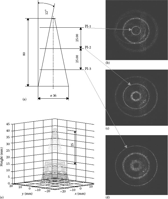
FIGURE 7.12 Schematic of the rough metallic cone used for the investigation (a). Reconstruction of holograms at three different planes separated by 25 mm (b through d). Numerical reconstruction of a part of the cone shape (e). (From Körner, K. et al., Opt. Express, 20(7), 7237, 2012.)

7.5.3 DIGITAL HOLOGRAPHIC INTERFEROMETRY

One of the most significant applications of classical holography is holographic interferometry, which was first developed in 1965 by Stetson and Powell [62,63]. This technique makes it possible to measure displacement, deformation, and vibration of rough surface with an accuracy of a fraction of a micrometer. It has been extensively used for metrological application since it allows the interferometric comparison of wavefronts of different states of the object that are not present simultaneously. In classical holographic interferometry, two or more holograms of the object under investigation are recorded usually by a photographic plate. The subsequent interference of these wave fields when they are physically reconstructed produces a fringe pattern, from where the information of the deformations or change of refraction index of the object between the exposures can be obtained. There exists a large literature describing the applications of classical holographic interferometry; particularly recommended are the books from C. Vest W. Schumann, Jones, and Wykes [64,65,66]. Electronic speckle interferometry (ESPI) [67,68] allowed to avoid the processing of films, which represents the major disadvantage of classical holographic interferometry. In the first ESPI systems, a vidicon device recorded the interference between light reflected by a diffusing object and a reference wave, but starting from 1980, CCDs and CMOS devices were used leading to a dramatic improvement of the results. ESPI and digital holographic interferometry are very similar techniques; both can use in-line [69] or off-axis [70,71] arrangement. The only difference is that for ESPI, the object is imaged on the recording device, and thus, a reconstruction by digital calculation of the wavefront propagation is not necessary. When the interferograms are digitally recorded (ESPI or digital holography), the phase of the wavefront can be determined by processing the intensity pattern, and the comparison between wavefronts recorded at different times is easy and fast. Digital holography has been extensively used for the measurement of deformations of large and microscopic objects [72,73,74,75], vibrations analysis [76,77,78,79,80,81], defect recognition [82], contouring [83], particle size and position measurements [84], and for the investigation of the change of refraction index of liquids and gases [85]. Here, we will show some results where the technique has been used to measure deformations.

7.5.3.1 Measurement of Object Deformations

We consider two digital holograms of the object recorded on two separate frames of a CCD or CMOS detector: the first one with the object in its initial state and the second one after the object has undergone a deformation that shifts the optical phase compared to the one in the first recording. Denoting the two digitally reconstructed wave fields with U_O1 and U_O2, respectively, their phases ϕ_o1 and ϕ_o2 can be directly calculated:

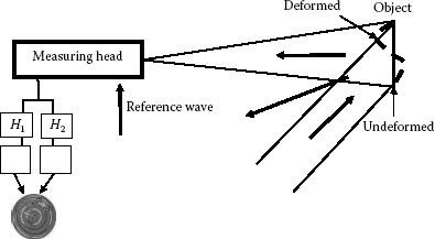
FIGURE 7.13 Digital holographic interferometry.

$ϕ_{o j} (m Δ x, n Δ y) = \arctan [\frac{Im [U_{o j} (m Δ x, n Δ y)]}{Re [U_{o j} (m Δ x, n Δ y)]}],$ $ϕ_{o j} (m Δ x, n Δ y) = \arctan [\frac{Im [U_{o j} (m Δ x, n Δ y)]}{Re [U_{o j} (m Δ x, n Δ y)]}],$

(7.24)

where j = 1, 2. ϕ_o1 and ϕ_o2 are wrapped phases (0 < ϕ_oj < 2π), and their difference

$Δ ϕ_{w} = ϕ_{o 2} - ϕ_{o 1}$ $Δ ϕ_{w} = ϕ_{o 2} - ϕ_{o 1}$

(7.25)

needs to be processed in order to eliminate the 2π incertitude and obtain Δϕ. The relation between the deformation $\vec{d}$ $\vec{d}$ of an arbitrary point of the surface and the phase change is

$Δ ϕ = \frac{2 π}{λ} \vec{d} \cdot \vec{s} .$ $Δ ϕ = \frac{2 π}{λ} \vec{d} \cdot \vec{s} .$

(7.26)

The vector $\vec{s} = {\vec{k}}_{o} - {\vec{k}}_{i}$ $\vec{s} = {\vec{k}}_{o} - {\vec{k}}_{i}$ (where ${\vec{k}}_{o}$ ${\vec{k}}_{o}$ and ${\vec{k}}_{i}$ ${\vec{k}}_{i}$ are the unit vectors of observation and illumination, respectively) is referred to as the sensitivity vector, which is given by the geometry of the recording arrangement. It lies along the bisector of the angle between the illumination and viewing directions. Equation 7.26 is the basis of all quantitative deformation measurements of solid objects by holographic interferometry. Figure 7.13 shows the recording geometry and the procedure for obtaining the phase difference from two digitally recorded holograms H₁ and H₂.

A single measurement yields one vector component of the deformation $\vec{d}$ $\vec{d}$ (projection to the sensitivity vector). In general, for determining the full 3D deformation vector $\vec{d}$ $\vec{d}$ , we need to perform at least three measurements with different sensitivity vectors $({\vec{s}}_{1}, {\vec{s}}_{2}, {\vec{s}}_{3})$ $({\vec{s}}_{1}, {\vec{s}}_{2}, {\vec{s}}_{3})$ . For each sensitivity vector, the phase difference (Δϕ₁, Δϕ₂, Δϕ₃) between the two deformation states is evaluated, and the 3D deformation field is determined by decomposing the sensitivity vectors into their scalar components and solving a linear system of equations [79].

7.5.3.2 Pulsed Digital Holographic Interferometry for the Measurement of Vibration and Defect Recognition

Figure 7.14 illustrates the measurement of a vibrating plate having a diameter of 15 cm. The plate was excited at the resonance frequency of 4800 Hz by using a shaker. A pulsed ruby laser, which emits two high-energy short pulses (pulse width 20 ns) separated by few microseconds, has been used for the recording of the two holograms on a CCD; in this specific case, the pulse separation was 10 μs. The measuring head consists of an off-axis arrangement with lens as shown in Figure 7.7, where the object was directly imaged on the CCD. The two digital holograms were processed, and their phase difference is shown in Figure 7.14a. By using an unwrapping procedure, it was possible to obtain the vibration shape shown in Figure 7.14b. The sensitivity vector was parallel to the observation direction, and the out-of-plane vibration of the plate was measured.

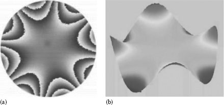
FIGURE 7.14 Plate (15 cm diameter) vibrating at 4800 Hz. Phase map (a) and pseudo-3D representation (b).

Figure 7.15 shows another example where pulsed digital holography interferometry has been used to investigate a metal plate submitted to a shock. The laser pulses were fired shortly after the shock produced by a metal ball fell on the plate. After calculation and subtraction of the phases of the two reconstructed digital holograms, we obtain a phase map with concentric fringes around the point of the impact. The shock wave propagating at the surface of the plate is disturbed by a small defect that can be clearly seen in the phase map. This shows the principle for defect detection in mechanical components.

The acquisition speeds of the CCD and CMOS semiconductor detectors have increased continuously (cameras recording 5000 image/s with a resolution of 500 × 500 pixels are commercially available), and methods for measuring dynamic events have been developed in which a sequence of digital holograms are recorded on a high-speed sensor. By unwrapping the phase in the temporal domain, it is possible to retrieve the displacement of an object as a function of time. The use of highspeed cameras for the investigation of dynamic events is reported in Refs. [86,87,88,89,90].

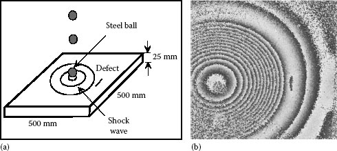
FIGURE 7.15 Object submitted to a shock excitation (a). Phase map obtained by double pulse exposure digital holography (b). (From Tiziani, H.J. et al., Interferometry, in: Landolt-Börnstein New Series, Laser Physics and Applications, Springer-Verlag, Berlin, Germany, 2006, pp. 221–284.)

7.5.3.3 Digital Holographic Interferometry for the Investigation of Microsystems

The trend toward miniaturization of micro-electro-mechanical systems (MEMS) and micro-opto-electro-mechanical systems continues to lead to more and more compact devices [91]. Applications cover a wide range of fields, from optical telecommunications to medicine; furthermore, MEMS-based accelerometers and pressure sensors are used in the aeronautical and automotive industry. Part of the functionality and reliability of MEMS devices is based on the displacement and deformation of micromechanical parts under mechanical, thermal, magnetic, or electrostatic loads. The measurement of the shape and deformation of such systems is thus of great importance for confirming analytical and finite element models, accessing material and device properties, detecting potential defects, and determining performance [92,93,94,95]. These data can then be used in further device optimization. Since typical structures exhibit dimensions in the order of some micrometers, it is necessary to measure their deformation with accuracies down to the lower nanometer range. Digital holography allows measurements of nanometric deformations and is thus well suited for the characterization of the micro devices.

A system is described in Ref. [96] to precisely determine the deformation of MEMS; the setup uses a stabilized laser and high-quality optical components with antireflection coating and was fixed on a vibration-isolated table. The CCD camera used has low noise and high dynamics (12 bits). The test object was the MEMS shown in Figure 7.16, designed to have a very accurate out-of-plane displacement (parallel to the observation direction) produced by applying an electrical voltage to the structure. Notice that the process of loading by applying a voltage to the MEMS and the acquisitions of the digital holograms are synchronized and done dynamically. Figure 7.16b through d shows 3D representations of the measured out-of-plane deformations when 15, 30, and 50 V are applied to the MEMS shown in Figure 7.16a. In order to compare the results, we consider the deformation at the center of the moving element as a function of the applied voltage. In Figure 7.17a and b, it is not possible to see any difference between measured (+) and expected (solid line) deformations. Their difference is reported in Figure 7.17c; the standard deviation is 1.4 nm, thus very small compared with the total deformation of 2 μm.

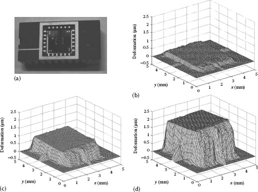
FIGURE 7.16 Photo (a) and out-of-plane deformations of a MEMS obtained by applying 15 V (b), 30 V (c), and 50 V (d). (From Pedrini, G. et al., Opt. Eng., 50, 101504-1, 2011.)

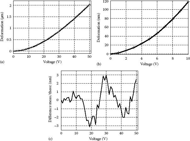
FIGURE 7.17 (a) Measured (+) and expected (solid line) deformation as a function of the applied voltage; (b) detail of (a); (c) difference between measured and expected results. (From Pedrini, G. et al., Opt. Eng., 50, 101504–1, 2011.)

REFERENCES

1. D. Gabor, A new microscopic principles, Nature, 161, 777–778 (1948).

2. E. N. Leith, J. J. Upatnieks, Wavefront reconstruction with diffused illumination and three-dimensional objects, Opt. Soc. Am., 54, 1295 (1964).

3. G. W. Stroke, An Introduction to Coherent Optics and Holography, 2nd edn., Academic Press, New York (1969).

4. H. M. Smith, Principles of Holography, Wiley-Interscience, New York (1969).

5. H. J. Caulfield, S. Lu, The Applications of Holography, Wiley-Interscience, New York (1970).

6. M. Lehmann, Holography, Technique and Practice, The Focal Press, London, U.K. (1970).

7. R. J. Collier, C. B. Burckhard, L. H. Lin, Optical Holography, Academic Press, New York (1971).

8. J. N. Butters, Holography and Its Technology, Peter Peregrinus Ltd., Published on behalf of the Institution of Electrical Engineering, London, U.K. (1971).

9. W. T. Cathey, Optical Information Processing and Holography, John Wiley & Sons, New York (1974).

10. B. R. Brown, A. W. Lohmann, Complex spatial filtering with binary masks, Appl. Opt., 5, 967–969 (1966).

11. J. W. Goodman, R. W. Lawrence, Digital image formation from electronically detected holograms, Appl. Phys. Lett., 11, 77–79 (1967).

12. J. W. Goodman, Digital image formation from holograms: Early motivation modern capabilities, in: Adaptive Optics: Analysis and Methods/Computational Optical Sensing and Imaging/Information Photonics/Signal Recovery and Synthesis Topical Meetings on CD-ROM, OSA Technical Digest (CD), paper JMA1, Optical Society of America, Washington, DC (2007).

13. M. A. Kronrod, N. S. Merzlyakov, L. P. Yaroslavskii, Reconstruction of a hologram with a computer, Sov. Phys. Tech. Phys., 17, 333–334 (1972).

14. L. P. Yaroslavskii, N. S. Merzlyakov, Methods of Digital Holography, Consultants Bureau, New York (1980).

15. W. S. Haddad, D. Cullen, J. C. Solem, J. W. Longworth, A. McPherson, K. Boyer, C. K. Rhodes, Fourier-transform holographic microscope, Appl. Opt., 31, 4973–4978 (1992).

16. Y. Takaki, H. Ohzu, Fast numerical reconstruction technique for high-resolution hybrid holographic microscopy, Appl. Opt., 38, 2204–2211 (1999).

17. G. Pedrini, P. Froning, H. J. Tiziani, F. Mendoza-Santoyo, Shape measurement of microscopic structures using digital holograms, Opt. Commun., 164, 257–268 (1999).

18. G. Pedrini, S. Schedin, H. J. Tiziani, Aberration compensation in digital holographic reconstruction of microscopic objects, J. Mod. Opt., 48, 1035–1041 (2001).

19. L. Xu, X. Peng, J. Miao, A. K. Asundi, Studies of digital microscopic holography with applications to microstructure testing, Appl. Opt., 40, 5046–5051 (2001).

20. I. Yamaguchi, J. Kato, S. Ohta, J. Mizuno, Image formation in phase-shifting digital holography and applications to microscopy, Appl. Opt., 40, 6177–6185 (2001).

21. G. Pedrini, H. J. Tiziani, Short-coherence digital microscopy by use of a lensless holographic imaging system, Appl. Opt., 41, 4489–4496 (2002).

22. W. Xu, M. H. Jericho, I. A. Meinertzhagen, H. J. Kreuzer, Digital in-line holography of microspheres, Appl. Opt., 41, 5367–5375 (2002).

23. M. Gustafsson, M. Sebesta, B. Bengtsson, S. G. Pettersson, P. Egelberg, T. Lenart, High-resolution digital transmission microscopy: A Fourier holography approach, Opt. Lasers Eng., 41, 553–563 (2004).

24. D. Carl, B. Kemper, G. Wernicke, G. Von Bally, Parameter optimized digital holographic microscope for high resolution living cell analysis, Appl. Opt., 43, 6536–6544 (2004).

25. P. Marquet et al., Digital holographic microscopy: A noninvasive contrast imaging technique allowing quantitative visualization of living cells with subwavelength axial accuracy, Opt. Lett., 30(5), 468–470 (2005).

26. B. Kemper, G. von Bally, Digital holographic microscopy for live cell applications and technical inspection, Appl. Opt., 47(4), A52–A61 (2008).

27. A. Anand, V. K. Chhaniwal, B. Javidi, Imaging embryonic stem cell dynamics using quantitative 3-D digital holographic microscopy, IEEE Photon. J., 3(3), 546–554 (2011).

28. B. Kemper et al., Label-free quantitative cell division monitoring of endothelial cells by digital holographic microscopy, J. Biomed. Opt., 15(3), 036009 (2010).

29. S. Witte et al., Short-coherence off-axis holographic phase microscopy of live cell dynamics, Biomed. Opt. Express, 3(9), 2184–2189 (2012).

30. F. Dubois et al., Partial spatial coherence effects in digital holographic microscopy with a laser source, Appl. Opt., 43(5), 1131–1139 (2004).

31. Y. Park et al., Speckle-field digital holographic microscopy, Opt. Express, 17(15), 12285–12292 (2009).

32. F. Dubois, P. Grosfils, Dark-field digital holographic microscopy to investigate objects that are nanosized or smaller than the optical resolution, Opt. Lett., 33(22), 2605–2607 (2008).

33. F. Verpillat et al., Dark-field digital holographic microscopy for 3D-tracking of gold nanoparticles, Opt. Express, 19(27), 26044–26055 (2011).

34. M. K. Kim, Principles and techniques of digital holographic microscopy, SPIE Rev., 1(1), 018005 (2010).

35. P. Marquet, B. Rappaz, P. J. Magistretti, E. Cuche, Y. Emery, T. Colomb, C. Depeursinge, Digital holographic microscopy: A noninvasive contrast imaging technique allowing quantitative visualization of living cells with subwavelength axial accuracy, Opt. Lett., 30, 468–470 (2005).

36. J. Garcia-Sucerquia, W. Xu, S. K. Jericho, P. Klages, M. H. Jericho, H. J. Kreuzer, Digital in-line holographic microscopy, Appl. Opt., 45, 836–850 (2006).

37. T. Colomb, F. Montfort, J. Kühn, N. Aspert, E. Cuche, A. Marian, F. Charrière, S. Bourquin, P. Marquet, C. Depeursinge, Numerical parametric lens for shifting, magnification, and complete aberration compensation in digital holographic microscopy, J. Opt. Soc. Am. A, 23, 3177–3190 (2006).

38. A. Faridian, G. Pedrini, W. Osten, High-contrast multilayer imaging of biological organisms through dark-field digital refocusing, J. Biomed. Opt., 18(8), 086009 (2013).

39. G. Pedrini, F. Zhang, W. Osten, Digital holographic microscopy in the deep (193 nm) ultraviolet, Appl. Opt., 46, 7829–7835 (2007).

40. A. Faridian et al., Nanoscale imaging using deep ultraviolet digital holographic microscopy, Opt. Express, 18(13), 14159–14164 (2010).

41. U. Schnars, Direct phase determination in hologram interferometry with use of digitally recorded holograms, J. Opt. Soc. Am. A, 11, 2011–2015 (1994).

42. G. Pedrini, Y. L. Zou, H. J. Tiziani, Digital double pulse-holographic interferometry for vibration analysis, J. Mod. Opt., 42, 367–374 (1995).

43. U. Schnars, Th. Kreis, W. P. Jueptner, Digital recording and numerical reconstruction of holograms: reduction of the spatial frequency spectrum, Opt. Eng., 35(4), 977–982 (1996).

44. G. Pedrini, Ph. Froening, H. Fessler, H. J. Tiziani, In-line digital holographic interferometry, Appl. Opt., 37, 6262–6269 (1998).

45. G. Pedrini, S. Schedin, H. Tiziani, Lensless digital-holographic interferometry for the measurement of large objects, Opt. Comm., 171, 29–36 (1999).

46. G. Pedrini, H. J. Tiziani, Digital holographic interferometry, in: Digital Speckle Pattern Interferometry and Related Techniques, P. K. Rastogi, ed., Wiley, Chichester (2001), pp. 337–362.

47. L. Yaroslavsky, Digital Holography and Digital Image Processing: Principles, Methods, Algorithms, Kluwer Academic Publishers, Boston (2004).

48. U. Schnars, W. Jueptner, Digital Holography: Digital Hologram Recording, Numerical Reconstruction, and Related Techniques, Springer, Berlin, Germany (2005).

49. Th. Kreis, Handbook of Holographic Interferometry (Optical and Digital Methods), Wiley-VCH, Weinheim, Germany (2005).

50. Th. Kreis, Holographic Interferometry, Principles and Methods, Akademie Verlag, Berlin, Germany (1996).

51. W. Goodman, Introduction to Fourier Optics, McGraw-Hill, New York (1996).

52. F. Zhang, I. Yamaguchi, L. P. Yaroslavsky, Algorithm for reconstruction of digital holograms with adjustable magnification, Opt. Lett., 29, 1668–1670 (2004).

53. I. Yamaguchi, T. Zhang, Phase-shifting digital holography, Opt. Lett., 22, 1268–1270 (1997).

54. W. Osten, N. Reingand, Optical Imaging and Metrology, Wiley-VCH, Berlin (2010).

55. T. Dresel, G. Häusler, H. Venzke, Three-dimensional sensing of rough surfaces by coherence radar, Appl. Opt., 31, 919–925 (1992).

56. B. Nilsson, T. E. Carlsson, Direct three-dimensional shape measurement by digital-in-flight holography, Appl. Opt., 37, 7954–7959 (1998).

57. J. Schmitt, Optical coherence tomography (OCT): A review, IEEE J. Sel. Top. Quantum Electron., 5, 1205–1215 (1999).

58. G. Indebetouw, P. Klysubun, Optical sectioning with low coherence spatio-temporal holography, Opt. Commun., 172, 25–29 (1999).

59. E. Cuche, P. Poscio, C. Depeursinge, Optical tomography by means of a numerical low-coherence holographic technique, J. Opt., 28, 260–264 (1997).

60. L. Martínez-León, G. Pedrini, W. Osten, Applications of short-coherence digital holography in microscopy, Appl. Opt., 44, 3977–3984 (2005).

61. K. Körner, G. Pedrini, I. Alexeenko, T. Steinmetz, R. Holzwarth, W. Osten, Short temporal coherence digital holography with a femtosecond frequency comb laser for multi-level optical sectioning, Opt. Express, 20(7), 7237–7242 (2012).

62. R. L. Powell, K. A. Stetson, Interferometric vibration analysis by wavefront reconstructions, J. Opt. Soc. Am., 55, 1593–1598 (1965).

63. K. A. Stetson, R. L. Powell, Interferometric hologram evaluation and real-time vibration analysis of diffuse objects, J. Opt. Soc. Am., 55, 1694–1695 (1965).

64. C. M. Vest, Holographic Interferometry, John Wiley & Sons, New York (1979).

65. W. Schumann, M. Dubas, Holographic Interferometry, Springer Verlag, Heidelberg, Germany (1979).

66. R. Jones, C. Wykes, Holographic and Speckle Interferometry, 2nd edn., Cambridge University, Cambridge, U.K. (1989).

67. J. N. Butters, J. A. Leendertz. Holographic and video techniques applied to engineering measurement, J. Meas. Control, 4, 349–354 (1971).

68. A. Macovski, D. Ramsey, L. F. Schaefer, Time lapse interferometry and contouring using television systems, Appl. Opt., 10, 2722–2727 (1971).

69. K. Creath, Phase-shifting speckle interferometry, Appl. Opt., 24, 3053 (1985).

70. G. Pedrini, B. Pfister, H. J. Tiziani, Double pulse electronic speckle interferometry, J. Mod. Opt., 40, 89–96 (1993).

71. G. Pedrini, H. J. Tiziani, Double-pulse electronic speckle interferometry for vibration analysis, Appl. Opt., 33, 7857 (1994).

72. U. Schnars, W. P. O. Juptner, Digital recording and reconstruction of holograms in hologram interferometry and shearography, Appl. Opt., 33, 4373 (1994).

73. C. Wagner, S. Seebacher, W. Osten, W. Jüpner, Digital recording and numerical reconstruction of lensless Fourier holograms in optical metrology, Appl. Opt., 38, 4812–4820 (1999).

74. S. Sebacher, W. Osten, W. Jueptner, Measuring shape and deformation of small objects using digital holography, Proc. SPIE, 3479, 104–115 (1998).

75. S. Seebacher, W. Osten, T. Baumbach, W. Jüptner, The determination of material parameters of microcomponents using digital holography, Opt. Laser Eng., 36, 103–126 (2001).

76. G. Pedrini, H. Tiziani, Y. Zou, Digital double pulse-TV-holography, Opt. Laser Eng., 26, 199–219 (1997).

77. G. Pedrini, Y. Zou, H. J. Tiziani, Simultaneous quantitative evaluation of in-plane and out-of-plane deformations using multi directional spatial carrier, Appl. Opt., 36, 786–792 (1997).

78. G. Pedrini, H. J. Tiziani, Quantitative evaluation of two dimensional dynamic deformations using digital holography, Opt. Laser Tech., 29, 249–256 (1997).

79. S. Schedin, G. Pedrini, H. J. Tiziani, F. M. Santoyo, Simultaneous three-dimensional dynamic deformation measurements with pulsed digital holography, Appl. Opt., 38, 7056–7062 (1999).

80. C. Perez-Lopez, F. Mendoza Santoyo, G. Pedrini, S. Schedin, H. J. Tiziani, Pulsed digital holographic interferometry for dynamic measurement of rotating objects with an optical derotator, Appl. Opt., 40, 5106–5110 (2001).

81. H. J. Tiziani, N. Kerwien, G. Pedrini, Interferometry, in: Landolt-Börnstein New Series, Laser Physics and Applications, Springer-Verlag, Berlin, Germany (2006), pp. 221–284.

82. S. Schedin, G. Pedrini, H. J. Tiziani, A. K. Aggarwal, M. E. Gusev, Highly sensitive pulsed digital holography for built-in defect analysis with a laser excitation, Appl. Opt., 40, 100–103 (2001).

83. G. Pedrini, Ph. Fröning, H. J. Tiziani, M. E. Gusev, Pulsed digital holography for high speed contouring employing the two-wavelength method, Appl. Opt., 38, 3460–3467 (1999).

84. M. Adams, Th. Kreis, W. Jueptner, Particle size and position measurements with digital holography, in: Optical Inspection and Micromeasurements, Ch. Gorecki, ed., Proceedings of SPIE, The International Society for Optical Engineering, Vol. 3098 (1997), pp. 234–240.

85. P. Gren, S. Schedin, X. Li, Tomographic reconstruction of transient acoustic fields recorded by pulsed TV holography, Appl. Opt., 37, 834–840 (1998).

86. G. Pedrini, I. Alexeenko, W. Osten, H. Tiziani, Temporal phase unwrapping of digital hologram sequences, Appl. Opt., 42, 5846–5854 (2003).

87. G. Pedrini, W. Osten, M. E. Gusev, High-speed digital holographic interferometry for vibration measurement, Appl. Opt., 45, 3456–3462 (2006).

88. G. Pedrini, W. Osten, Time resolved digital holographic interferometry for investigations of dynamical events in mechanical components and biological tissues, Strain, 43(3), 240–249 (2007).

89. Y. Fu, G. Pedrini, W. Osten, Vibration measurement by temporal Fourier analyses of a digital hologram sequence, Appl. Opt., 46, 5719–5727 (2007).

90. Y. Fu, R. M. Groves, G. Pedrini, W. Osten, Kinematic and deformation parameter measurement by spatiotemporal analysis of an interferogram sequence, Appl. Opt., 46, 8645–8655 (2007).

91. J. Korvink, O. Paul, eds., MEMS: A Practical Guide to Design, Analysis and Applications, William Andrew Publishing, Norwich, NY (2006).

92. W. Osten, ed., Optical Inspection of Microsystems, CRC Press, Boca Raton, FL (2006).

93. W. Osten, ed., Optical microsystems metrology—Part I, Opt. Lasers Eng., 36, 75 (2001).

94. W. Osten, ed., Optical microsystems metrology—Part II, Opt. Lasers Eng., 36, 401 (2001).

95. G. Coppola, P. Ferraro, M. Iodice, S. De Nicola, A. Finizio, S. Grilli, A digital holographic microscope for complete characterization of microelectromechanical systems, Meas. Sci. Technol., 15, 529–539 (2004).

96. G. Pedrini, J. Gaspar, M. Schmidt, I. Alekseenko, O. Paul, W. Osten, Measurement of nano/micro out-of-plane and in-plane displacements of micromechanical components by using digital holography and speckle interferometry, Opt. Eng., 50, 101504-1–101504-10 (2011).

..................Content has been hidden....................

You can't read the all page of ebook, please click here login for view all page.

Table of Contents for Chapter 7 Holography

Create new playlist

Sign In

Sign Up

Table of Contents for
Chapter 7 Holography