
CONTENTS
16.2.1 Homodyne Interferometer and Heterodyne Interferometer
16.2.2 Optical System of an Interferometer
16.2.3 Factors That Effect the Measurement Result and Uncertainty
16.2.3.1 Refractive Index of Air
16.2.3.2 Stability of the Dead Path
16.2.3.3 Unbalanced Optical Path Lengths and Thermal Change
16.3.1.1 Incremental Type and Absolute Type
16.3.2 Methods of Scale Mark Detection
16.3.2.2 Image Transmission Scale Encoders
16.3.2.3 Diffraction Scale Encoders
16.3.2.4 Hologram Scale Encoders
16.3.3 Direction of Linear Encoders
16.3.4 Calibration of Linear Encoders
16.4.4 Optical Frequency Sweep Method
16.4.5 Air Refractivity for Distance Measurement
Measurement of displacement is important for precise positioning, processing, and testing. Typical optical techniques for the measurement of displacement use equipment such as laser interferometers, linear encoders, and distance meters. This chapter introduces these measurement techniques.
A laser interferometer measures displacement using interferometry. It is widely used in areas such as lithography, precision machine processing, and coordinate measuring machines due to its noncontact, high-speed, and high precision-measurement features.
16.2.1 HOMODYNE INTERFEROMETER AND HETERODYNE INTERFEROMETER
Most laser interferometers have the same configuration as the Michelson interferometer. One of the reflecting mirrors of the Michelson interferometer is attached to the object whose displacement is to be measured. The two main types of laser interferometers are the homodyne type and the heterodyne type.
Consider two linearly polarized light waves on photodetectors E1 and E2, whose polarization directions are the same and optical frequencies are f1 and f2, respectively. These waves are expressed by
where
V1 and V2 are the amplitudes
ϕ1 and ϕ2 are the phases of the waves
The interference signal between the two light waves is expressed by
The case of f1 = f2 is referred to as a homodyne interferometer. The displacement is measured by the change in the phase of the interference signal. The fluctuation of the DC level of the interference signal that is caused by the change of laser power, for example, deteriorates the accuracy of the phase measurement. The interferometer developed by National Physical Laboratory takes three interference signals whose phases are 0°, 90°, and 180° respectively and eliminates DC component by combining these signals [1]. This interferometer is therefore robust to DC level fluctuation.
When f1 ≠ f2, a beat signal with a beat frequency of |f1 – f2| is observed. The case is referred to as a heterodyne interferometer. If the reflecting mirror moves, the light reflected by the mirror undergoes a Doppler shift. When the light with the optical frequency of f2 is reflected by the moving mirror with a velocity of v, the Doppler shift Δf2 is 2vf2/c, where c is the speed of light. The number of waves counted during time T is 2vT(f2/c) = 2L/λ2, where L is the displacement and λ2 is the wavelength of light with frequency f2.
For precise interferometry, the stability of the laser frequency is important. The two frequencies are usually generated by a two-mode stabilized laser, a Zeeman laser, an acousto-optic modulator (AOM), or a pair of AOMs. The beat frequency is ~600 MHz in the case of a He–Ne two-mode stabilized laser, in the range of a few hundred kilohertz to a few megahertz in the case of a Zeeman laser and several tens of megahertz in the case of an AOM. A higher beat frequency means a faster measurable movement speed.
16.2.2 OPTICAL SYSTEM OF AN INTERFEROMETER
Figure 16.1 shows the heterodyne-type laser interferometer used to measure the displacement of a corner reflector [2,3,4]. Light beams with different frequencies, f1 and f2, are linearly polarized, and the directions of polarization are orthogonal to each other. In order to make the reference beat signal with a frequency of |f1 – f2|, portions of the light beams are reflected by a beam splitter (BS). These light beams pass through a polarizer with a direction of 45° and generate the beat signal on a photodetector. The remaining light beams are incident on a polarization beam splitter (PBS). The reflected light by PBS, whose optical frequency is f1, traverses the fixed path with a stable corner reflector and is reflected by the PBS again. The transmitted light with an optical frequency of f2 traverses the changing path with a moving corner reflector and is transmitted to the PBS. These two beams interfere and generate a beat signal on another photodetector after passing through a polarizer. The phase difference between the measurement beat signal and reference beat signal indicates the displacement of the moving corner reflector.
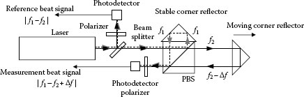
FIGURE 16.1 Heterodyne-type laser interferometer for the displacement measurement of a corner reflector. PD: photodetector.
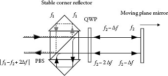
FIGURE 16.2 Heterodyne-type laser interferometer for the displacement measurement of a plane mirror. QWP: quarter-wave plate.
A corner reflector is useful because it reflects the light beam back in the same direction without feedback to the laser light source. However, some applications require the use of a plane mirror instead of a corner reflector. The configuration shown in Figure 16.2 is often used in the case of a plane mirror [5]. By changing the polarization direction of the measurement beam with a quarter-wave plate (QWP), the measurement beam traverses a measurement path twice. As a result, the resolution is doubled compared to that of a corner reflector.
16.2.3 FACTORS THAT EFFECT THE MEASUREMENT RESULT AND UNCERTAINTY
16.2.3.1 Refractive Index of Air
The refractive index of air should be taken into account when optical interferometry is used for the measurement of length. There are two methods for the correction of the refractive index of air. One is to measure the environmental conditions such as air temperature, air pressure, humidity, and density of carbon dioxide. An empirical equation is then used to calculate and correct the refractive index of air [6]. The other method is to use a length-stabilized cavity, the so-called wavelength tracker [7,8]. The wavelength tracker consists of a stable cavity and a differential interferometer, as illustrated in Figure 16.3. One polarization component traverses the optical path that is reflected from the front surface of the etalon, and the other is reflected on the back surface. This differential interferometer measures the optical length of the cavity. The cavity is made of a low thermal-expansion material and its geometric length is very stable; therefore, the change in the optical length of the cavity is considered to be the result of the change in the refractive index of air inside the cavity. The change in the refractive index of air is measured by monitoring the optical length of the cavity, and can then be used for the correction of displacement measurement conducted in the same environment.
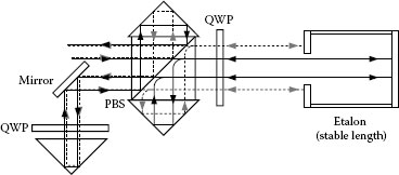
FIGURE 16.3 Schematic representation of a wavelength tracker.
16.2.3.2 Stability of the Dead Path
The temperature change along the reference and measurement paths induces error. Most commercial laser interferometers set the reference mirror or corner reflector near the beam splitter so that alignment is easier and the measurement is more robust to environmental changes. The distance from the beam splitter to the closest limit of the displacement range is called the dead path, as shown in Figure 16.4. The dead path has no role in the displacement measurement, however, it does have an effect on the measurement results, that is, the fluctuation in the optical length of the dead path caused by temperature change or vibration induces an error in the measurement result.
16.2.3.3 Unbalanced Optical Path Lengths and Thermal Change
The optical length is the product of the refractive index and the geometric thickness. The temperature dependence of the refractive index of general optical glass is larger than that of air. For example, when the total path lengths in the glass of the reference and measurement paths are not balanced due to the use of wavelength plates, the temperature change may have an effect on the result. To avoid an imbalance of the path lengths, optical systems such as that shown in Figure 16.5 are used [9]. In Figure 16.2, the optical path length of the measurement light beam in the PBS is twice that of the reference light beam, while the optical path lengths of the measurement and reference light beams in the PBS are the same in the optical system of Figure 16.5.
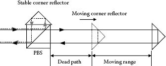
FIGURE 16.4 Schematic representation of the dead path. PBS: polarizing beam splitter.
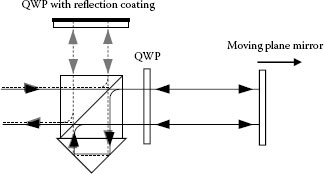
FIGURE 16.5 Interferometer used to balance the optical path lengths.
The measurement system should be coaxial to the length to be measured, according to the Abbe principle. If the measurement laser beam is shifted by d from the moving axis whose displacement is to be measured, then an error, which is called the Abbe error, is induced by the angular error of movement, as shown in Figure 16.6. If the translation stage has a rotation error of θ, then the Abbe error, δ, is d × sin θ.
When the measurement axis is not parallel to the moving axis, a cosine error is induced. Alignment of the measurement and moving axes should be performed by moving the corner reflector or reflecting mirror as much as possible in order to minimize the cosine error.
Imperfections of antireflection coatings, polarization optics, and polarization alignment may induce contamination with unwanted reflections or the leakage of polarization in the measurement signal. The phase of the detected signal is not linear to the actual displacement in this case. There are several reports regarding the avoidance of nonlinear errors by spatially separating the light beams [10,11].
The progress of nanotechnology has increased the demand for sub-nanometer displacement measurements and the calibration of such measurement systems. Two-beam interferometers suffer from nonlinear errors and have difficulty achieving sub-nanometer range uncertainties. Techniques that use the Fabry–Perot cavity are attractive for measurements with picometer-order uncertainty over a small range, such as in the order of micrometers. In this technique, the optical frequency of a tunable laser is locked to one of the resonance modes of the Fabry–Perot cavity. The displacement of one of the mirrors, which is the quantity to be measured, causes a change in the resonant frequency of the mode. By measuring the resonant frequency change, the small displacement of the mirror can be precisely measured. The tuning range of the laser limits the measurable range of the displacement. There have been several attempts to expand the measurable displacement range, for example, using successive resonant modes of the cavity [12], optical frequency comb generators [13], and femto-second-comb wavelength synthesizers [14].
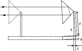
FIGURE 16.6 Schematic representation of Abbe error.
A linear encoder usually consists of a scale unit, signal converting and interpolating unit, and an indicator (Figure 16.7). The scale unit includes a scale (or tape) that has marks to indicate the distance or position, and a reading head that detects the marks. A reading head usually includes optical source and optical system. The mark detection signal is converted to an electrical signal, interpolated by a counter in the interface unit, and then the displacement information is output to the indicator. A schematic diagram of the linear encoder is given in Figure 16.8.
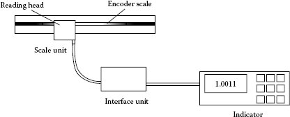
FIGURE 16.7 Example of linear encoder configuration.
In practical use, such as in the manufacturing industries, linear encoders other than laser interferometers are commonly used for positioning. Linear encoders are more convenient than laser interferometers in manufacturing, because they do not require complicated alignment of optics, and the resolution of linear encoders has improved; the resolution of recent linear encoders is of the same order or better than that of laser interferometers. Linear encoders also have a feature in that they are insusceptible to environmental fluctuations. Moreover, the encoder “encodes” the displacement of the scale and outputs a digital signal, as its name suggests. The output digital signal can be used to measure the position and operation of the working system. This feature has resulted in the widespread use of encoders in manufacturing and machine tools.
Rotary encoders detect the angle of a ball screw rotation, and the position of the stage can be calculated from the number of rotations. However, linear encoders directly detect the displacement by detecting the number of graduations on a scale using the reading head. This reason also improves the usefulness of linear encoders.
There are several kinds of linear encoders. The magnetic-scale type and the magnet–electric type are the oldest types of linear encoders. They have scales with tiny magnet graduations on it. The resolutions of the magnetic type and the magnet–electric type are limited by the spacing of magnets on the scale tape. The optical scale has overcome the limit by making fine marks on glass using micro-fabrication technologies. We concentrate on the optical type linear encoders according to the concept of this book.
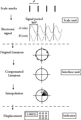
FIGURE 16.8 Process of displacement measurement by a linear encoder.
There are various kinds of optical linear encoders, which are categorized by their appearance: enclosed type (shield type) and exposed type. Enclosed-type linear encoders are mainly used for positioning in machining tools, because they are resistant to dirt or oil contaminants found in the factories due to their enclosing shield. However, exposed-type linear encoders are mainly used in the clean rooms of high-technology industries. Therefore, the resolutions of the exposed-type linear encoders are usually high, about 1 nm. The scale of optical linear encoders is usually made of glass with graduations made of evaporated chromium or gratings on it. There are also different concept exposed-type optical encoders; the long-scale measuring type. The long-scale type has exposed tape scale, which is made of metal and reading head. The resolutions of this type of encoders are not so high compared to the high-resolution-type exposed encoders. However, these types of encoders are used for large dimension manufacturing because the tape can be made longer, and attachment to the machining tool is easier than that for the enclosed type.
The measurement principles of linear encoders with glass scale, details of scale mark detection, view for the near future, and calibration of linear encoders are explained in the following subsections.
The scale marks of glass-scale optical linear encoders are made of etched metals, gratings, holographic gratings, etc. The optical source for the optical linear encoders is light-emitting diode (LED) or laser diode (LD). An optical source such as LED or LD and a photodetector are usually built into one reading head. Light that is transmitted, reflected, or diffracted by the scale is detected by the photodetector in the reading head. The intensity of detected light generates a sinusoidal signal (in-phase signal) and the different sinusoidal signal, which has 90° offset signal (quadrature signal). From the two 90° phase-shifted signals, cyclic signals, such as sinusoidal signals or transistor–transistor logic (TTL) signals, are synthesized [15]. The cyclic signal usually has distortion and noise caused by contamination or manufacturing errors of the scale. The cyclic signal with distortion and noise is compensated to a true cyclic signal electrically or by processor, after which, the cyclic signal is interpolated. The signal period of interpolated signal is the resolution of the encoder. Interpolation technology is just as important as the optical system. The interpolation number reaches 4000, therefore, increasing the S/N ratio is a significant issue.
16.3.1.1 Incremental Type and Absolute Type
The incremental-type linear encoder has equal interval marks (or periodic marks) on the scale. The detector in the reading head counts the number of marks the reading head passed through. The distance that the reading head moved, x, is calculated from the interval of marks, d, and the number of marks the reading head passed through, m, as x = dm.
Because the absolute position cannot be determined using a primitive incremental-type linear encoder, the origin points are also usually placed on the scale. The absolute position can then be determined by calculating the distance from the origin point. However, this requires an additional process, in that the reading head must go back to the origin point, at the beginning of each measurement.
The absolute-type linear encoder provides the position of the reading head. The absolute-type encoder has equal interval (or periodic) marks on the scale, in addition to serial-absolute-code marks that indicate the absolute position on the scale. Using the serial absolute code marks, the detector can identify the absolute position without passing through the origin point.
Optical linear encoders are categorized by their scale-marking method. The basic type is the image transmission (shutter) type, which uses two scales with slits, a main scale and an index scale. The interval of the slits is about 10 μm. The intensity of the light that passes through the two slits is detected and converted to displacement information.
Diffraction type scale marking is also commonly used, and generally, the resolution is better than the image transmission type. In this type, a diffraction grating is ruled on the scale. The incident light is diffracted by the scale and interferes at the detector. The grating pitch can reach 5 μm using lithographic techniques. In high-resolution-type diffraction encoders, the light beam passes through the slits twice before reaching the detector, and is thus diffracted twice, which allows the resolution to be increased by four times compared to the single diffraction.
The highest resolution is realized by the hologram type, which uses a hologram scale to diffract the light. A hologram grating is memorized using a laser source with almost the same wavelength as the encoder light source, ~0.55 μm. In this type, double diffraction is also used, and the resolution of the detected signal is increased by four times compared with the grating pitch. The period of the detected signal is 0.138 μm.
16.3.2 METHODS OF SCALE MARK DETECTION
The Moiré method uses two scales that have different pitch marks. Marks spaced with a pitch of p1 are on the main scale, and on the index scale the marks are spaced with a slightly different pitch of p2. Parallel light is formed using a condenser lens, passes through the index scale and the main scale, and is then detected by a photodetector. At the detector, the Moiré fringe is detected, which corresponds to the pitch of the scales. When the main scale displaces by p1 – p2, the Moiré fringe displaces by p1p2/(p1 – p2), and the displacement of the scale can be measured by counting the Moiré fringe.
In Moiré scale encoders, the diffracted light and interference of the diffracted light becomes larger as the mark pitch becomes finer. To avoid contamination of the signal by diffraction, the index scale must be set closer to the main scale in proportion to the square of the mark pitch. The limit of the mark pitch is approximately 10 μm.
16.3.2.2 Image Transmission Scale Encoders
An image transmission scale encoder (Figure 16.9) has an index scale and a main scale with marks of the same pitch [16]. When the light is aligned, the light passes through both, the index scale and main scale, and the intensity of light detected by the photodetector is high. When the marks on the index scale overlap the gap on the main scale, no light passes through the scales, and the intensity of light detected by the photodetector is low. In this type of scale, the displacement of the scale is determined by detecting the intensity of light that passes through the scales. In this case, an LED is used as the light source. In a commercial image transmission scale, other marks on the index scale and another photodetector generate quadrature signal, and therefore, the direction of the movement of the scale can be determined [16,17]. The image transmission scale has an advantage in that it is robust to an incline of the reading head, including an incline of the index scale to the main scale. For the same reason as with the Moiré scale, the limit of the scale pitch is determined by diffraction limit and the distance of the index scale and main scale; 20–40 μm. There are several types of commercially available image transmission scales; the limit of resolution of these types of scales is 0.05 μm.
16.3.2.3 Diffraction Scale Encoders
Diffraction scale encoders have a diffraction grating on the main scale, the index scale, or both of these scales. The light from an LD is diffracted by the grating on the main scale, passes through the index scale, and is then detected by the photodetector. The light diffracted by the diffraction grating on the main scale makes a Fresnel diffraction pattern on the index scale. When the bright pattern is matched to the interval of marks on index scale, the intensity of the light detected by the photodetector is high. Movement of one of the scales causes the intensity of the light to become sinusoidal. This method actively utilizes diffracted light to detect the displacement of the scale. The main scale pitch of commercial encoders is 8 or 5 μm.
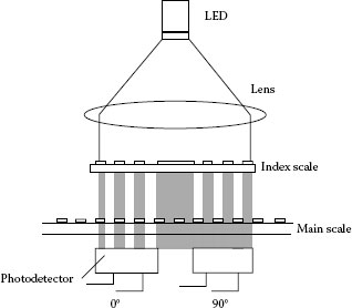
FIGURE 16.9 Optical system of an image transmission scale encoder.
16.3.2.4 Hologram Scale Encoders
Hologram scale encoders use a hologram diffraction grating on the scale. The light beam from an LD is divided into two optical paths using a PBS, and is incident on the hologram scale. The hologram grating is held between two glass plates in order to avoid blurs or scratch.
Magnescale Co., Ltd. developed a hologram scale encoder using only one scale with a hologram diffraction grating having a pitch of 0.55 μm; almost the same length as the wavelength of the light source (Figure 16.10) [18]. One of the beams, which is going in the right direction, is diffracted to the left direction by the grating. The diffracted light is then reflected by a mirror and goes back to the grating and the PBS. Two times diffraction by the grating results in the phase of the light being shifted by Δϕr = 4πx/p, where x is the displacement of the scale and p is the grating pitch. The other beam, which is going in the left direction, is diffracted two times and the phase is shifted by Δϕl = −4πx/p. The two beams interfere at the beam splitters in front of the photodetectors. The intensity of the interference signal changes sinusoidally by the displacement of the scale. The period of intensity change is 8πx/p, four times larger than one period of phase change. The period of the detected signal is p/4, a four-cycle phase change corresponding to the displacement of the scale by one grating pitch, p. Since the grating pitch is 0.55 μm, the signal pitch is 0.14 μm.
Four photodetectors are used to detect the interference signal. A quarter-wave plate (QWP) and half mirror cause the interfered beam to split into two signals with 90° different phases. By subtracting the reverse phase signals from the four photodetectors, a sine signal and a cosine signal with a 0.14 μm period are electrically induced. Using the resistive divider and an A/D converter, the sine and cosine signals are interpolated 4000 times. The resolution of this encoder is 0.034 nm. This hologram grating scale encoder has not only high resolution but also robustness for vibration, fluctuations of air, and air pressure changes because it is a bilaterally symmetric optical system.
16.3.3 DIRECTION OF LINEAR ENCODERS
According to the current trend for miniaturization of semiconductor manufacturing, sizes of the processing scale have already entered the nanometer scale; therefore, higher resolution is demanded for linear encoders. A linear encoder that has a 34 pm resolution is already commercially available.
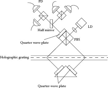
FIGURE 16.10 Optical system of a hologram scale encoder.
However, other trends of developing linear encoders are influenced by features such as convenience of use, environmental resistance, and minimization. Enclosed-type encoders, in which the scale is enclosed in a case and assembled with the reading head, are suitable for use in factory and general industrial environments, where oil or dirt contaminants are common. Absolute measurement type rather than the incremental type encoders are increasing according to the usefulness of absolute type; the absolute encoders do not require the process of passing through the original point.
To make machine tools smaller or to speed up the movement of the stage or machine by reducing weight, minimization of linear encoders is also demanded. Smaller optical components and smaller optical systems are being developed to make the reading head smaller. A reading head in which the optical system and interpolating circuit are mounted together has already been developed.
For real-time measurement in high-speed manufacturing, optical linear encoders that are applicable for reading speeds faster than 3 m/s are used.
16.3.4 CALIBRATION OF LINEAR ENCODERS
As the resolution of linear encoders is increasing, the demand for calibration of linear encoders is also increasing. The resolution of general linear encoders is in the order of 1 nm; the highest resolution of linear encoders has reached 34 pm (34 × 10−12 m). These high-resolution linear encoders are widely used in cutting-edge industries, such as semiconductor manufacturing, optical disk exposure, and high-precision processing. In these industries, the traceability of measurements is a strict requirement with the advance of globalization; therefore, precise calibration of these encoders is very important.
There are various types of linear encoders with different shapes of scales, shapes of reading head, types of optical system, and different types of signal processing for the various scales. This variety makes the development of a calibration system rather difficult. At present, the calibration systems used for linear encoders are individual systems from each manufacturer.
Comparative calibration methods are usually used by the encoder manufacturers in the encoder-manufacturing process or for the product inspection. The encoder that is to be calibrated is set on the measurement bed adjacent to the master standard linear encoder. The reading heads of the calibrated and reference linear encoders are fixed to a movable stage on the bed. As the movable stage displaces, both the encoders measure the displacement. The calibrated encoder can be calibrated compared to the master standard encoder. The reference standard encoder is calibrated by laser interferometer once a year or every several months. In this comparative method, Abbe’s principle cannot be satisfied, because the two encoders cannot be set on the same space. Therefore, the Abbe error is compensated by calculating the space difference between the two encoders, and the straightness of the movable stage. The measurement uncertainty of these comparators is generally on the order of 100 nm.
Laser interferometers are used for absolute measurement of linear encoders for the calibration of master linear encoders used for standard manufacturing in factories or calibration laboratories, or in national metrology institutes. Figure 16.11 shows a schematic diagram of the absolute calibrator for linear encoders at the National Metrology Institute of Japan. This calibrator uses a double-pass laser interferometer with a resolution of 1.2 nm. The calibrated linear encoder is set on the center of two corner cubes to satisfy Abbe’s condition. The calibration system is covered by an insulation box, and the air temperature fluctuation inside the box is passively stabilized to 50 mK. Air temperature, air pressure, humidity, and the density of carbon dioxide are measured for compensation of the refractive index of air. The scale temperature is also measured and used to compensate for the thermal expansion coefficient. The measurement range is up to 1000 mm. Using this calibrator, the measurement uncertainty is 50 nm (k = 2) for encoders with 350 mm length and 1.2 nm resolution.
Vacuum interferometers are the outstanding calibration systems for linear encoders. By encapsulating the optical path of the interferometers of calibrator into a vacuum, fluctuations in the refractive index of air become significantly smaller, so that the uncertainty caused by the calibration system becomes small. The uncertainty of the linear encoder calibration system used at Physikalisch-Technische Bundesanstalt (PTB) has already reached 10 nm for a 600 mm scale [19,20].
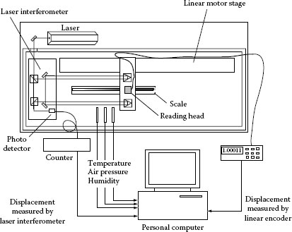
FIGURE 16.11 Scheme of the absolute calibrator of linear encoder in the National Metrology Institute of Japan.
For higher resolution linear encoders, better than approximately 1 nm resolution, several methods of calibration are under development. The accuracy of laser interferometers is limited to approximately 1 nm due to the nonlinearity error. New concepts and ideas for the prevention of nonlinearity in laser interferometers or methods other than laser interferometer are necessary.
At the National Physical Laboratory, United Kingdom, a sub-nanometer calibrator has been developed by combining an optical laser interferometer and an x-ray interferometer [21]. This system uses a silicon lattice as a sub-nanometer graduation. Although in these x-ray interferometer systems sub-nanometer resolution is realized, there are the problems of safety of x-ray and the large size of the x-ray system. The feature that the resolution is determined by the average lattice spacing also makes a problem for the direct calibration of linear encoders in real time.
With regard to direct traceability and real-time calibration, sub-nanometer calibration systems based on laser interferometers are in high demand, and several systems are under development [13,22].
Distance is defined as a quantity between two separate points. Although the definition is essentially independent of value, the word distance is also frequently used to mean “long length.” In this subsection, we describe how to optically measure lengths over approximately a few meters.
Distance measurements are classified into two types. One is the measurement of a value between two points, and the other is a measurement of a change in long length. The former is an absolute length and the latter a displacement. Optical measurements have an advantage in their fine scale, that is, wavelength. The wavelengths of light range from several hundred nanometers to several micrometers. Moreover, smaller lengths can be obtained by measuring the phase of an interfering fringe. However, this “fine scale” also has a disadvantage in distance measurements, especially in absolute distance measurements, because the wavelengths are too small to measure distances.
For this reason, wavelength is not generally used as a scale for absolute distance measurements. However, wavelength is usually used as a scale for displacement measurements of long lengths. In this case, long baseline interferometers and/or long baseline optical resonators are used. For example, laser strain meters that have observed ground motion and laser interferometer gravitational wave detectors are in existence. With regard to laser strain meters, a 100 m baseline Michelson interferometer has been operated in Kamioka, Japan [23]. An example of a gravitational wave detector, Fabry–Perot cavity interferometers with a 4 km baseline have been operated in the United States [24]. The largest interferometer has been planned as a space gravitational wave detector with a baseline of 5,000,000 km [25]. These large interferometers and long resonators are placed in a vacuum, because variation of the air refractivity limits the sensitivity of optical distance measurements. The influence of air refractivity on distance measurements is described in the following subsection. Although special techniques and knowledge are required for the construction of large interferometers, the principle is the same as that for small or conventional size interferometers. Therefore, we will not give a detailed description of long length displacement measurements, but will describe in detail the measurement of absolute distance.
The most easily understood concept of distance measurements is the method of time of flight of a light pulse. A pulse of light is sent and a receiver receives the pulse. The time difference between sending and receiving provides information on the distance that the light pulse has traveled. Distance can be calculated by dividing the speed of light by the time taken. An illustration of this scheme is shown in Figure 16.12. The resolution of the measured distance is limited by the time resolution. If the time can be measured with a resolution of 1 ns, then the distance can be determined with a resolution of 30 cm. This method is useful in roughly long distance measurements.
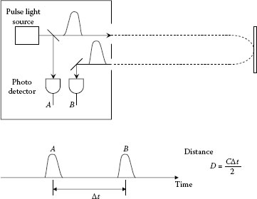
FIGURE 16.12 Diagram of distance meter using pulse method.
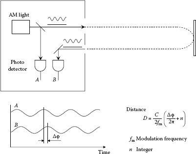
FIGURE 16.13 Diagram of distance meter using modulation method.
A method that uses amplitude modulated light is usually used in distance measurements. This method is based on phase-sensitive detection. The optical configuration is shown in Figure 16.13. Light to which amplitude modulation (AM) is added or which originally had amplitude modulation is divided into two paths. One is the reference path, which has a short path to a photodetector, and the other travels the measurement path and is detected by another photodetector. The phase difference between the two modulated light detected by each photodetector provides information on the measurement path length. Almost all electric distance meters (EDMs) used for surveying employ this method. For example, when the modulation frequency is 50 MHz, the amplitude modulation wavelength is approximately 6 m. As the light travels both ways between the EDM and the target, the phase is turned 360° with a distance of 3 m. By accurately measuring the phase, some EDMs have a resolution of 0.1 mm. In order to obtain information of an integer multiple of the half modulation wavelength, commercially available EDMs use methods to switch to multi-modulation frequency or to sweep modulation frequency.
Higher modulation frequency, that is, smaller modulation wavelength, may provide better distance resolution. A special EDM with a modulation frequency of 28 GHz and distance resolution of a few micrometers has been developed [26]. Another special EDM has been developed, which has a femto-second laser as the light source [27]. One of the features of a femto-second laser is its ultra-stable repetition rate, which means that a femto-second laser has an amplitude modulation that is a combination of fundamental and higher orders of repetition frequency. If the repetition frequency is 50 MHz, then the femto-second laser has amplitude modulations of 50 MHz, 100 MHz, 150 MHz, …, 10 GHz, …. By extracting only one frequency component of the electric signal, for example 10 GHz, this is the same system as the EDM with a sinusoidal wave of the frequency.
16.4.4 OPTICAL FREQUENCY SWEEP METHOD
In this method, the optical frequency of the light source is continually changed. From the optical frequency of the returned light that was reflected by a target, we can know when the light went out. Generally, the optical frequency is changed using a serrodyne waveform. The light is separated into a short reference path and the measurement path. The light through the reference path and the light through measured path are combined by the beam splitter. The combined light has a beat signal whose frequency is the difference of optical frequencies between the reference light and the measured light. An illustration of the method is given in Figure 16.14 and the calculation is made using the following equation:
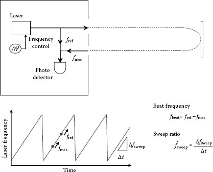
FIGURE 16.14 Diagram of distance meter using serrodyne sweep method.
where
D is the measured distance
c is the speed of light
fbeat is the frequency of the beat signal
fsweep is the frequency sweep rate
The beat frequency should be measured during the time range in which the optical frequency monotonically changes. If the measured distance is fixed, a constant beat frequency is obtained. The frequency is dependent on the sweep rate of the optical frequency at the slope on the serrodyne waveform. Features of this system are quick measurements and high resolution. This method is used in coordinate measuring equipment known as Laser Tracker® (Leica Geosystems).
16.4.5 AIR REFRACTIVITY FOR DISTANCE MEASUREMENT
Almost all distance measurements in air are limited in their accuracy by air refractivity. The refractive index of air is close to 1.00027 under standard conditions of air. The value of air refractivity is changed by the wavelength of light, air temperature, air pressure, humidity, and the density of carbon dioxide. Air temperature and air pressure have a significant effect on the change of air refractivity, and their factors are approximately 1 ppm/K and 0.3 ppm/hPa, respectively. Air pressure can be regarded as unity in horizontal distance measurements. However, air temperature is different at any spatial point within the measurement area. Therefore, it is necessary to have a large number of thermometers in order to determine the correct average temperature of the air along the measured optical path. Therefore, it is difficult to measure a long distance in air with good accuracy, especially outdoors.
Regarding the speed of the measurement light, it should be noted that in the modulation method, the modulated light travels with the speed of a group velocity in air. It is several parts per million (ppm) or more than a dozen ppm slower than the phase velocity. The refractive index is equal to the value obtained by dividing the speed of light by the phase velocity in air. Similarly, the value obtained by dividing the speed of light by a group velocity is sometimes referred to as a “group refractive index.” This word is expediently used with regard to length measurements in air, notwithstanding that it is an incorrect word. It is because the law of group refraction is nonexistent!
As previously remarked, it is difficult to exactly determine the environmental parameters in long distance measurements. Two color measurements can measure a distance without measuring environmental parameters such as temperature, pressure, humidity, and the density of carbon dioxide. Since differential coefficients of the refractive index for environmental parameter are dependent on the wavelength of light, the values of the refractive index of air can be determined for each wavelength from the difference of two wavelength measurements. The refractive indexes of air as a function of air temperature at wavelengths of 532 and 1064 nm, and the respective differences, are shown in Figure 16.15.
Let us define two words, “geometrical distance” and “optical distance.” Geometrical distance is defined as the true distance between two points. Optical distance is defined as the distance that includes refractivity, that is, it is the product of geometrical distance multiplied by the refractive index of air. The equation of the two color measurement is given as
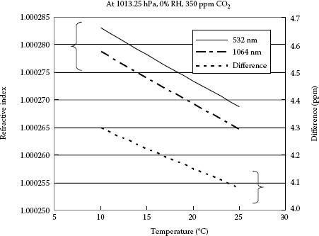
FIGURE 16.15 Air refractivity and difference of air refractivity.
where
D is the geometrical distance
L1 and L2 are the optical distances for wavelengths 1 and 2, respectively
A is an essential parameter in two color measurements and is expressed as
where n(λ1) and n(λ2) are the refractive indexes of air for wavelength 1 and 2, respectively. If the humidity is 0%, then the value of A is constant and independent of the other environmental parameters. Thus, the geometrical distance can be determined without measuring the environmental parameters. If humidity is not 0%, the value of A is not exactly constant, but is regarded as being almost constant. Although it is advantageous that the environmental parameters need not be measured, there is a disadvantage in the two color distance measurements. The value of A is several tens to one hundred, and depends on the two wavelengths. From Equation 16.5, we know that the accuracy of the geometrical distance is A times worse than that of measured optical distances. For this reason, the two color measurement is useless for short distance or short length measurements.
1. Downs, M.J. and Raine, K.W., An unmodulated bi-directional fringe-counting interferometer system for measuring displacement, Prec. Eng., 1, 85, 1979.
2. Laser and Optics User’s Manual, Chap. 7A, Linear interferometers and retroreflectors, Agilent Technologies, 2002, http://literature.cdn.keysight.com/litweb/pdf/05517-90108.pdf (accessed January 20, 2015).
3. Wuerz, L.J. and Quenelle, R.C., Laser interferometer system for metrology and machine tool applications, Prec. Eng., 5, 111, 1983.
4. Demarest, F.C., High-resolution, high-speed, low data age uncertainty, heterodyne displacement measuring interferometer electronics, Meas. Sci. Technol., 9, 1024, 1998.
5. Laser and Optics User’s Manual, Chap. 7C, Plane mirror interferometer, Agilent Technologies, 2002, http://literature.cdn.keysight.com/litweb/pdf/05517-90110.pdf (accessed January 20, 2015).
6. Ciddor, P.E., Refractive index of air: New equations for the visible and near infrared, Appl. Opt., 35, 1566, 1996.
7. Siddall, G.J. and Baldwin, R.R., Developments in laser interferometry for position sensing, Prec. Eng., 6, 175, 1984.
8. Laser and Optics User’s Manual, Chap. 7I, Wavelength tracker, Agilent Technologies, 2002, http://literature.cdn.keysight.com/litweb/pdf/05517-90116.pdf (accessed January 20, 2015).
9. Achieving Maximum Accuracy and Repeatability, Product Note, Agilent Technologies, 2001, http://literature.cdn.keysight.com/litweb/pdf/5952-7973.pdf (accessed January 20, 2015).
10. Wu, C.-M., Lawall, J., and Deslattes, R.D., Heterodyne interferometer with subatomic periodic nonlinearity, Appl. Opt., 38, 4089, 1999.
11. Lawall, J. and Kessler, E., Michelson interferometry with 10 pm accuracy, Rev. Sci. Instrum., 71, 2669, 2000.
12. Haitjema, H., Schellekens, P.H.J., and Wetzels, S.F.C.L., Calibration of displacement sensors up to 300 mm with nanometer accuracy and direct traceability to a primary standard of length, Metrologia, 37, 25, 2000.
13. Bitou, Y., Schibli, T.R., and Minoshima, K., Accurate wide-range displacement measurement using tunable diode laser and optical frequency comb generator, Opt. Exp., 14, 644, 2006.
14. Schibli, T.R. et al., Displacement metrology with sub-pm resolution in air based on a fs-comb wavelength synthesizer, Opt. Exp., 14, 5984, 2006.
15. Nagai, R., Saito, H., and Ueda, M., Present and future technology of ultraprecision positioning, Chapter 5, p. 2, Fuji Technosystems Co., Ltd. 2000 (in Japanese).
16. Magnescale Co., Ltd., http://www.mgscale.com.
17. Heidenhain Corp., http://www.heidenhain.com.
18. Mitutoyo Corp., http://www.mitutoyo.co.jp/eng/.
19. Tiemann, I. et al., An international length comparison using vacuum comparators and a photoelectric incremental encoders as transfer standard, Prec. Eng., 32, 1, 2008.
20. Flugge, J., Koning, R., and Bosse, H., Recent activities at PTB nanometer comparator, Recent developments in traceable dimensional measurements II, Proc. SPIE, 5190, 391, 2003.
21. Leach, R., Haycocks, J., Jackson, K., Lewis, A., Oldfield, S., and Yacoot, A., Advances in traceable nanometrology at the National Physical Laboratory, Nanometrology, 12, R1, 2001.
22. Kajima, M. and Matsumoto, H., Calibration of linear encoders with sub-nanometer uncertainty using an optical-zooming laser interferometer, Prec. Eng., 38, 769, 2014.
23. Takemoto, S. et al., A 100 m laser strainmeter system installed in a 1 km deep tunnel at Kamioka, Gifu, Japan, J. Geodynamics, 38, 477, 2004.
24. Waldman, S.J. et al., Status of LIGO at the start of the fifth science run, Class. Quantum Grav., 23, S653, 2006.
25. Danzmann, K. et al., LISA technology—Concept, status, prospects, Class. Quantum Grav., 20, S1, 2003.
26. Fujima, I., Iwasaki, S., and Seta, K., High-resolution distance meter using optical intensity modulation at 28 GHz, Meas. Sci. Technol., 9, 1049, 1998.
27. Minoshima, K. and Matsumoto, H., High-accuracy measurement of 240-m distance in an optical tunnel by use of a compact femtosecond laser, Appl. Opt., 39, 5512, 2000.