18	Flatness
	Toshiyuki Takatsuji and Youichi Bitou

CONTENTS

18.1    Introduction

18.1.1    Definition of Flatness

18.2    Interferometric Flatness Measurements

18.2.1    Fizeau Interferometer

18.2.1.1    Principle of Operation of a Phase-Shifting Fizeau Interferometer

18.2.1.2    Methods to Determine the Surface Profile of a Reference Flat

18.2.1.3    Error Sources in a Phase-Shifting Fizeau Interferometer

18.2.1.4    Fizeau Interferometer in Practical Applications

18.2.2    Oblique Incidence Interferometer

18.3    Flatness Measurement Using Angle Sensors

18.3.1    Contact-Type Flatness Measurement System Using Angle Sensors

18.3.2    Noncontact-Type Flatness Measurement System Using Angle Sensors

18.3.2.1    Extended Shear Angle Difference Deflectometry

18.3.2.2    Long Trace Profiler

References

18.1    INTRODUCTION

Because flatness is one of the most important parameters that characterize optical properties of optical devices such as plane mirrors and prisms, a wide variety of measuring techniques has been invented so far. The simplest method is observing the curvature of the interference fringes formed between the sample and an optical flat. This method, however, is capable of measuring only λ/20 of the curvature, and it is not always sufficient for current applications.

Phase shifting method drastically enables more accurate measurement of the phase of the interference fringes. Additionally, the development of image processing devices and computers improves measurement accuracy as well as instrument facilitation. Under this condition, flatness measurement is becoming more important in industries. Quality inspection of not only optical devices but also silicon wafers, hard disk substrates, and flat panel displays requires accurate flatness measurement. There are other ultra-accurate applications, such as lithography mask for semiconductor manufacturing and optical devices for synchrotron facilities and gravitational wave observatories, and for these applications 1/100 wavelength or smaller measurement accuracy is needed.

In this section, various measurement principles of flatness measurement are introduced. Then, error factors and elimination methods are explained followed by the current situation of measurement uncertainty and traceability.

18.1.1    DEFINITION OF FLATNESS

According to the ISO standards, flatness is defined by the minimum zone method. This definition is practically suitable for mechanical engineering where surfaces of mechanical parts make physical contact with each other. It is not always easy to calculate the flatness from measurement data acquired using optical measuring instruments which are explained in this section.

The most common definition that is used in almost all instruments is based on the least square method. The least square plane is derived from the measurement data and the distance from this plane to each measurement data is calculated. Additionally, there are two definitions based on the least square method: P – V value and rms. The P – V value is the sum of the distances of two points that are the farthest from the least square plane on both sides. The rms is the root mean square of the distances of all measurement data from the least square plane.

The minimum zone flatness and the P – V flatness are not always the same value, and they have the following relation:

$\text{Minimum}\text{zone}\text{flatness}\le \text{P}-\text{V}\text{value}$

The P – V flatness and the rms flatness have the following relationship:

$\text{P}-\text{V}\text{value}\ge \text{rms}\text{value}$

The relation between the P – V and the rms varies for the form of the plane, and the P – V is often more than 10 times larger than the rms. When we discuss the value of the flatness, special caution should be taken for the definition of flatness.

SI unit is recommended to express flatness; however, the wavelength λ of the light source is often used such as λ/20. In this case, caution should be exercised for the value of λ. Recently, 632.8 nm (the wavelength of He–Ne laser) has been commonly used.

In addition to the expression of the value of flatness, the same expression such as λ/20 is used for that of measurement uncertainty (or error). In most cases, it is not clearly stated whether λ/20 means the range or ±λ/20 (=1/10 in range).

When the uncertainty is larger than the measurement value, the probable area where true measurement value exists extends to the negative region. No clear solution for this contradiction has been presented even in the field of metrology.

18.2    INTERFEROMETRIC FLATNESS MEASUREMENTS

Interferometry has been widely employed for optical testing including flatness. Using interferometry, we can obtain the two-dimensional surface profiles of test objects without scanning. Conventionally, a Newton interferometer using a lamp source has been used for practical flatness testing [1]. However, this method requires contact between a Newton standard and the test surface. In at least one case, damage occurred to the test surface as a result. Recently, laser interferometers have become popular for flatness testing because they can perform contact-free measurements.

18.2.1    FIZEAU INTERFEROMETER

18.2.1.1    Principle of Operation of a Phase-Shifting Fizeau Interferometer

A Fizeau interferometer has a simple optical configuration and is commonly used in practical flatness measurements. In a Fizeau interferometer, the interference fringe pattern between a reference flat and the measurement (test) flat is observed, and the phase distribution of the fringe pattern is calculated. A surface profile of the measurement flat can be determined from the calculated phase distribution.

Figure 18.1 shows the basic optical configuration of a Fizeau interferometer using a laser light source. A laser beam is collimated using an objective lens, pinhole, and collimating lens. A reference optical flat is oriented perpendicular to the collimated beam. The reference optical flat is made with a wedge or an antireflection (AR) coating to prevent reflection from its back surface. The interference fringe pattern between the reference and the measurement flats is detected using a television (TV) camera. A beamsplitter or a λ/4 plate and polarized beamsplitter are used to steer the beam to the TV camera. Alternatively, the reference flat can be set at a slight angle and a beamsplitter is not used [2]. In that type of Fizeau interferometer, a collimating lens with a long focal length is required to achieve high accuracy.

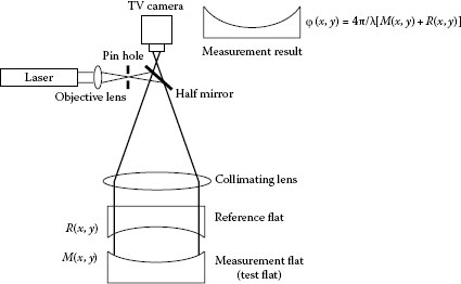
FIGURE 18.1  Configuration of a Fizeau interferometer.

Theoretically, the interference fringe pattern I(x, y) is

$I\left(x,y\right)=I_0\left\{1+\text{γ}\left(x,y\right)\cos \left[\phi \left(x,y\right)+{\phi }_0\right]\right\}$

(18.1)

where

I₀ is the background intensity

γ(x, y) is the fringe modulation

φ(x, y) is the phase distribution to be measured

φ₀ is the initial phase due to the optical path difference between the reference and the measurement surfaces

To obtain the phase distribution φ(x, y) from the interference fringe pattern I(x, y), the phase-shifting method is well used. In the phase-shifting method, the phase of a fringe is shifted by an optical path length change or a wavelength change. When an additional phase shift φ_i is given, the interference fringe pattern I_i(x, y) becomes

$I_i\left(x,y\right)=I_0\left\{1+\text{γ}\left(x,y\right)\cos \left[\phi \left(x,y\right)+{\phi }_0+{\phi }_i\right]\right\}$

(18.2)

where i is an integer. Theoretically, i is required to be larger than 3 in order to calculate the phase distribution φ(x, y). In the standard phase-shifting method, phase steps of 2π/j are used, where j ≥ 3 is an integer such that φ_i – φ_i–1 = 2π/j. In the most popular phase-shifting algorithm (called the four-step algorithm with i = j = 4), four interference fringe patterns with a π/2 phase step are used. In the four-step algorithm, the phase distribution φ(x, y) can be calculated as

$\phi \left(x,y\right)=\arctan \left[\left(I_2-I_4\right)/\left(I_1-I_3\right)\right]$

(18.3)

For achieving precise phase distribution, a high degree of phase step accuracy is required. To reduce measurement errors, phase-shifting algorithms with a large number of phase steps have been developed [3,4,5,6,7,8]. In actual applications, five- (i = 5, j = 4) or seven- (i = 7, j = 4) step algorithms are often used [3,7]. For example, in a typical five-step algorithm, the phase distribution φ(x, y) can be calculated as [3]

$\phi \left(x,y\right)=\arctan \left[2\left(I_2-I_4\right)/\left(2I_3-I_5-I_1\right)\right]$

(18.4)

The arctangent returns a phase value between 0 and 2π. There are discontinuities at 2π that must be corrected to obtain a usable result (phase unwrapping). The TV camera resolution must be at least two pixels per interference fringe period (according to the Nyquist theorem). Many types of unwrapping algorithms have been developed [9] and used in commercially available Fizeau interferometers.

The phase step is realized by an optical path length or wavelength change. A piezoelectric transducer (PZT) can vary the optical path length and is widely employed as a phase shifter in Fizeau interferometers. Although a PZT phase shifter is simple and easy to operate, it is difficult to obtain spatially uniform phase steps over a large aperture. Laser diodes (LDs) are useful light sources in a phase-shifting interferometer (PSI) because of their frequency tunability. The phase of the interference fringe in an unbalanced (Fizeau) interferometer is shifted by changing the LD frequency. Unlike in a PSI that uses a PZT, a PSI without moving parts and having a spatially uniform phase shift can be realized by tuning the frequency of an LD [10]. In both PZT and LD systems, special efforts must be made to calibrate the phase step values for high accuracy.

The surface profile M(x, y) of the measurement flat can be calculated from the phase distribution φ(x, y) as

$M\left(x,y\right)=\lambda /4\pi \times \phi \left(x,y\right)-R\left(x,y\right)$

(18.5)

where

λ is the wavelength of the laser source

R(x, y) is the surface profile of the reference flat

To obtain the surface profile M(x, y) of the measurement flat, we have to know not only the phase distribution φ(x, y) but also the surface profile R(x, y) of the reference flat. Generally, the flatness of the reference flat is better than λ/10 and we can neglect its surface profile R(x, y). However, for high-accuracy measurements (better than λ/20), the surface profile R(x, y) of the reference flat has to be known. Methods to determine the surface profile R(x, y) of the reference are described in the next section.

18.2.1.2    Methods to Determine the Surface Profile of a Reference Flat

For absolute flatness testing, the surface profile of the reference flat is needed. It can be determined using a liquid-flat reference [11] or a three-flat test [12].

A liquid surface can be used to determine the surface profile of another reference flat or it can be directly used as the reference flat in a Fizeau interferometer. Theoretically, the radius of curvature of a liquid surface is equal to that of Earth. For a diameter of 0.5 m, a phase value of the liquid surface can be estimated to better than λ/100 [1]. Mercury or oil is normally used as the liquid-flat reference [11]. But one of the main problems in a practical system is to isolate vibrations.

On the other hand, the three-flat test is frequently adopted in interferometric flatness measurement machines because the liquid-flat reference is difficult to realize practically. In the three-flat test, one prepares three similar flats (A, B, and C, including the target reference flat) and measures the phase distributions of every pair of flats (AB, AC, and BC). Figure 18.2 illustrates the concept behind the three-flat test. From the three measurements, one obtains the functions f_AB(x, y), f_AC(x, y), and f_BC(x, y) as

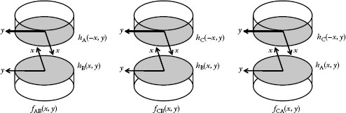
FIGURE 18.2  Three measurement combinations used in the three-flat test.

$\begin{array}{l}{h}_{\text{A}}\left(-x,y\right)+h_{\text{B}}\left(x,y\right)=f_{\text{AB}}\left(x,y\right)\hfill \\ h_{\text{C}}\left(-x,y\right)+h_{\text{B}}\left(x,y\right)=f_{\text{CB}}\left(x,y\right)\hfill \\ h_{\text{C}}\left(-x,y\right)+h_{\text{A}}\left(x,y\right)=f_{\text{CA}}\left(x,y\right)\hfill \end{array}$

(18.6)

where h_A(x, y), h_B(x, y), and h_C(x, y) are the surface profiles of A, B, and C, respectively. In the measurement procedure, one flat (A in Equation 18.6) has to be inverted across a flip axis (the y-axis in Equation 18.6). From Equation 18.6, we obtain the solution for profiles on the y-axis (at x = 0) as

$\begin{array}{l}{h}_{\text{A}}\left(0,y\right)=\left[f_{\text{AB}}\left(0,y\right)+f_{\text{CA}}\left(0,y\right)-f_{\text{CB}}\left(0,y\right)\right]/2\hfill \\ h_{\text{B}}\left(0,y\right)=\left[f_{\text{AB}}\left(0,y\right)+f_{\text{CA}}\left(0,y\right)-f_{\text{CB}}\left(0,y\right)\right]/2\hfill \\ h_{\text{C}}\left(0,y\right)=\left[-f_{\text{AB}}\left(0,y\right)+f_{\text{CA}}\left(0,y\right)-f_{\text{CB}}\left(0,y\right)\right]/2\hfill \end{array}$

(18.7)

To obtain the whole two-dimensional surface profiles h_A(x, y), h_B(x, y), and h_C(x, y), additional measurements with rotations of one surface is necessary [12] (as illustrated in Figure 18.3). One rotation angle θ is set to be 360°/n and the phase distributions with n rotational steps are measured, where n is an integer. In actual Fizeau interferometer systems, one rotation angle θ is fixed at between 10° and 30°. Several types of reconstruction algorithms have been developed [1,12,13,14,15,16]. Typically, the profiles for half of the rotation angle (corresponding to radial line data of h_C(r cos mθ/2, r sin mθ/2), where m is an integer) can be determined [16] and Zernike polynomials are then used to approximate the whole surface profiles. In some reconstruction algorithms, special approximations for the surface profiles and for the iteration calculations are adopted. For example, if the flat A satisfies the symmetry condition h_A(x, y) = h_A(–x, y), one can calculate the whole surface profiles h_A(x, y), h_B(x, y), and h_C(x, y) using Equation 18.6 alone.

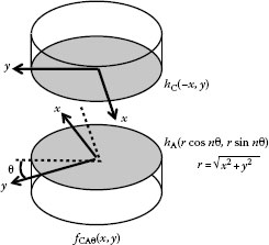
FIGURE 18.3  Rotation in the three-flat test.

18.2.1.3    Error Sources in a Phase-Shifting Fizeau Interferometer

Interferometric measurements are sensitive to environmental fluctuations. There are many kinds of systematic errors in a PSI. In this section, some of the principal sources of error are described.

18.2.1.3.1 Environmental Fluctuations

Mechanical vibrations and air turbulence are fundamental error sources in interferometric measurements. Using appropriate prevention systems such as a vibration absorbing table, environmental influences can be reduced to the nanometer or sub-nanometer level. To reduce air turbulence, the measurement and reference flats should be brought as close together as possible.

18.2.1.3.2 Phase-Shifting Errors

Systematic phase errors produce a non-sinusoidal waveform of the interference signal and a periodic error in the calculated phase profile. For example, in a practical Fizeau interferometer system using a PZT phase shifter, residual uncertainties in the phase shift remain because of the nonlinear response of a PZT to the applied voltage and thermal drift in the PZT. In addition, nonlinear response of the TV camera to the light intensity becomes an error source in a phase-shifting Fizeau interferometer [17].

For practical applications, the phase-shifting algorithm given by Equation 18.3 (four-step algorithm) is undesirable because of these errors. Several other kinds of phase-shifting algorithms have been developed instead. Even keeping the same number of phase steps, there are different kinds of algorithms [7,8]. The sensitivity to errors is different for each algorithm. But on the whole, phase-shifting algorithms that use a large number of phase steps are more effective at reducing the errors. Using an appropriate phase shifter and algorithm, one can attain a phase-shifting error of less than λ/100.

18.2.1.3.3 Determination of the Absolute Profile of a Reference Flat

In the three-flat test process, many interferometric measurements are required to determine the phase profile. In addition to the error sources described above, a gravity deformation effect is a serious problem in vertical Fizeau interferometers. In such an interferometer, both flats are equally deformed by gravity, as shown in Figure 18.4. Gravity deformations therefore cannot be observed and become an error source in the determination of the absolute profile of the reference flat. One solution to reduce this error is to analyze the gravity deformation numerically. Generally speaking, a reference flat has a simple figure and the value of the gravity deformation can be numerically estimated by computer simulation using a finite-element method [18]. The error due to the gravity deformation can then be reduced by compensating for the calculated value.

18.2.1.3.4 Mounting the Measurement Flat

For high-accuracy flatness measurements (better than λ/20), the mounting method becomes important. The surface profile depends on the figure of the base (for a vertical setting) or on the mounting method (for a horizontal setting). To reduce their influences, a thick plate (more than several centimeters) or an appropriate mounting method is desirable.

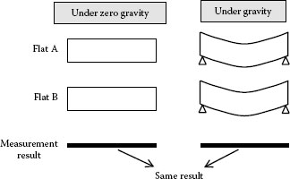
FIGURE 18.4  Influence of gravity deformations in a Fizeau interferometer.

18.2.1.3.5 Coherent Noise

In a laser interferometer system, unwanted interference fringes caused by reflections from the optical elements, such as the lenses, beamsplitter, and TV camera, become error sources in the measured phase profiles. Theoretically, fixed interference fringe noise does not influence the measurement result. However, in a PSI with an LD wavelength change, unwanted interference fringes are shifted and give rise to error in the measured phase profiles. To prevent this coherent noise problem, AR coatings on the optical elements or reduction of the spatial coherence using a rotating diffusion plate are effective. In addition, avoiding unwanted interference fringes from the TV camera is necessary [19].

18.2.1.4    Fizeau Interferometer in Practical Applications

18.2.1.4.1 National Standard Flatness Measurement Machine

Fizeau interferometers are often used as standard flatness measurement machines because of their high accuracy. Figure 18.5a through c shows photographs of the national standard Fizeau interferometer at the National Metrology Institute of Japan (NMIJ), the National Institute of Standards and Technology (NIST), and the Physikalische Technische Bundestadt (PTB), respectively. The absolute profiles of the reference flats in the NMIJ and NIST interferometers have been determined using the three-flat test and that in the PTB interferometer has been determined using a mercury liquid surface. The NIST Fizeau interferometer does not have a gravity deformation problem because it has a horizontal configuration. These three interferometers have a similar accuracy of around 10 nm for 250–300 mm diameter flats. The results of these interferometers guarantee the absolute accuracy of a practical flatness measurement machine and the tractability of flatness measurements [20].

18.2.1.4.2 Measurement of Optical Parallels

In a Fizeau interferometer, it is difficult to measure the surface profile of parallel plates because of unwanted interference fringes due to the back surface reflection, as shown in Figure 18.6a. One method to suppress the back reflection is to use index-matching oil on the back surface. Another method is wavelength-tuned phase-shifting interferometry. A special algorithm can selectively extract the correct interference signal from the noise-overlapped interference signal because the phase shifts of each fringe depend on the optical path difference [21,22]. A low-coherence interferometer provides a third method to remove the unwanted interference fringe due to the back surface reflection [23].

18.2.1.4.3 Measurement of an Optical Flat Having High Reflectivity

In a Fizeau interferometer, it is difficult to measure the surface profile of an optical flat having high reflectivity, such as an aluminum-coated mirror. When the reference plane is the glass surface and the reflectivity of the measurement flat is higher than that of the glass surface, the two reflected beam intensities become unbalanced, as shown in Figure 18.6b. In this case, the interference fringe contrast decreases and the measurement accuracy deteriorates. In addition, sinusoidal interference fringe signals are not observed and consequently, the interference signal is not given by Equation 18.1. The phase distribution calculated by the phase-shifting algorithm includes a systematic error.

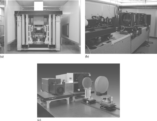
FIGURE 18.5  Photograph of the national standard Fizeau interferometer located at (a) NMIJ, (b) NIST, and (c) PTB.

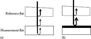
FIGURE 18.6  Measurement conditions for (a) optical parallels and (b) an optical flat having high reflectivity.

A simple method to increase the fringe contrast is to insert an absorption plate, although the phase distortion due to the absorption plate has to be compensated for in high-accuracy measurements. Another method to overcome this problem is to utilize a special coating that absorbs on the reference surface [24,25]. By utilizing such special coatings, high fringe contrast can be obtained even for reflectivities as high as 100%.

18.2.1.4.4 Fourier Transform Method for a Fizeau Interferometer

In a phase-shifting Fizeau interferometer, five or seven interference fringe images are required and so it is not suitable for rapid testing. For faster measurements such as of vibrations, a Fourier transform method is applicable because only one interference fringe image is used to calculate the phase distribution [26]. Typically, in a phase-shifting Fizeau interferometer, the number of interference fringes is set to as few as possible by adjusting the tilt angle between the reference and the measurement flats to reduce the phase-unwrapping error. In contrast, in the Fourier transform method, a spatial carrier fringe is added and the phase distribution is calculated for the carrier fringe. Note that a higher resolution is then required for the TV camera.

18.2.2    OBLIQUE INCIDENCE INTERFEROMETER

In Fizeau interferometry, the measurement sensitivity depends on the wavelength of the laser light source (usually sub-micrometer). For some practical applications, this sensitivity is too high to observe interference fringes. For example, in the flatness measurement with several tens of micrometer phase value, such as in the surface profile measurement of a silicon wafer, the spatial frequency of the interference fringes becomes higher than the resolution of the TV camera and it is difficult to measure the fringe images. In this case, an oblique incidence interferometer is useful [27,28]. Figure 18.7 shows the optical configuration of a typical oblique incidence interferometer. A collimated laser beam incident on grating 1 splits into two beams (due to zeroth- and first-order diffractions). The zeroth-order beam is used as the reference and the first-order beam is incident on the measurement flat at an angle Θ. The reflected beam from the measurement flat and the zeroth-order diffracted beam are combined by grating 2 and the interference fringes are observed on a screen. If the surface profile of the reference beam is negligibly small, the measured phase distribution φ′(x, y) is

${\phi }^{\prime }\left(x,y\right)=4\pi \cos \text{Θ}/\lambda \times M\left(x,y\right)$

(18.8)

In an oblique incidence interferometer, the measurement sensitivity is 1/2 cos Θ times that of a Fizeau interferometer. To calculate the phase distribution, the shifting of the interference fringes is needed; it is obtained by moving grating 1 or 2.

Another configuration of an oblique incidence interferometer uses a prism as the beamsplitter. The configuration of such an interferometer is shown in Figure 18.8. The reflection surface of the prism serves as the reference plane. The incident beam angle to the measurement flat can be changed and the measurement surface and the reference flat can be brought close together. However, it is difficult to manufacture a large prism.

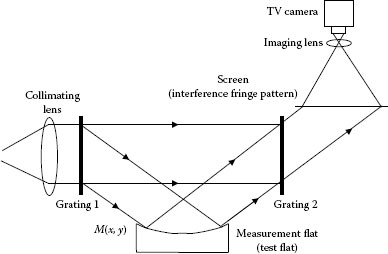
FIGURE 18.7  Configuration of an oblique incidence interferometer.

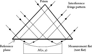
FIGURE 18.8  Configuration of an oblique incidence interferometer using a prism.

18.3    FLATNESS MEASUREMENT USING ANGLE SENSORS

Using interferometric methods, it is difficult to measure flatness over a diameter larger than 300 mm. One solution is to use angle sensors. Although a scanning operation is then required to obtain the two-dimensional surface profile, it is possible to expand the measurement range to over 1 m. Similar accuracy to that of a Fizeau interferometer is expected using precise angle sensors.

There are two kinds of angle sensor systems: a contact type and a noncontact type. Contact systems are simpler, while noncontact systems have been developed for ultraprecise surface profile measurements.

18.3.1    CONTACT-TYPE FLATNESS MEASUREMENT SYSTEM USING ANGLE SENSORS

Figure 18.9 shows a flatness measurement system using an autocollimator. In this system, a reflector is scanned across the measurement surface and the variation Δh(x) (i.e., local slope) of the surface profile h(x) is deduced from the reflection angle φ using the relation

$\tan \frac{\phi \left(x\right)}{2}=\frac{\text{Δ}h\left(x\right)}{D}$

(18.9)

where D is the length of the reflector. The surface profile h(x) can be obtained by integrating Equation 18.9. To obtain a two-dimensional surface profile, it is necessary to scan the reflector in two directions. This method is simple for in situ testing of flatness. However, the spatial resolution depends on the length D and so one cannot obtain high spatial resolution. Furthermore, the positioning uncertainty of the reflector causes a large measurement error and this method is not suitable for soft or thin materials, such as a silicon wafer. More simple method is to utilize a mechanical indicator.

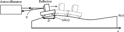
FIGURE 18.9  Configuration of a contact-type flatness measurement system using an autocollimator.

18.3.2    NONCONTACT-TYPE FLATNESS MEASUREMENT SYSTEM USING ANGLE SENSORS

In this section, two types of noncontact flatness measurement systems are introduced.

18.3.2.1    Extended Shear Angle Difference Deflectometry

Extended shear angle difference (ESAD) was developed for ultraprecise measurement of slope and topography of near-plane surfaces [29]. The configuration of the ESAD system is shown in Figure 18.10. A pentaprism deflects the autocollimator beam by 90° toward the surface of the measurement flat. The change in reflection angle is measured at points on the surface separated by lateral shears. The surface profile is reconstructed from two sets of angles measured by the autocollimator. To realize accurate results, a careful scanning method and integration algorithm have been developed [30,31]. The special resolution of this method depends on the value of the lateral shear and high resolution leads to long measurement times.

Unlike interferometric methods, the ESAD results do not depend on a reference surface. Instead, they depend on the accuracy of the angle and shear value measurements. A pentaprism is one of the key device to realize the high accuracy and long measurement range [32]. ESAD systems have achieved measurement ranges of over 1 m with sub-nanometer repeatability and can be expected to produce nanometer accuracy.

18.3.2.2    Long Trace Profiler

A long trace profiler (LTP) also relies on small-angle measurements. The configuration of such a LTP system is shown in Figure 18.11. The LTP measures the surface slope profile using a pencil beam interferometer [33]. In the LTP system, a pencil beam pair is created by an interferometer using two prisms, as shown in Figure 18.11. Two sets of pencil beam pairs are then made by a polarizing beam splitter and incident to the measurement flat and reference flat, which are rigidly mounted on the optical table, respectively. The beams from the measurement flat and reference flat do not interfere and the reference flat is used to compensate the mechanical error. Both sets of reflection beams are focused on a linear detector array, typically a CCD. On the linear detector array, interference spot patterns are observed. The variation in the surface slope due to the laser beam scanning is measured via the change in the interference spot position, detected using a linear array sensor. Laser beam scanning with small error is realized using a pentaprism, just as in the ESAD system [34]. The surface profile is reconstructed from the measured surface slope profile. The LTP can measure small angles with sub-microradian sensitivity and accuracy, and the surface profile with nanometer accuracy. In addition, both ESAD and LTP systems can measure aspheric profiles.

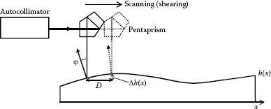
FIGURE 18.10  Geometry for ESAD deflectometry.

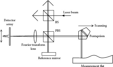
FIGURE 18.11  Configuration of an LTP.

REFERENCES

1.  Mantravadi, M. V., Newton, Fizeau, and Haidinger interferometers, in Optical Shop Testing, 2nd edn., Malacara, D. (Ed.), John Wiley & Sons Inc., New York, 1992, Chapter 1.

2.  Oreb, B. F., Farrant, D. I., Walsh, C. J., Forbes, G., and Fairman, P. S., Calibration of a 300-mm-aperture phase-shifter, Appl. Opt. 39, 5161, 2000.

3.  Hariharan, P., Oreb, B. F., and Eiju, T., Digital phase-shifting interferometry: A simple error-compensating phase calculation algorithm, Appl. Opt. 26, 2504, 1987.

4.  Larkin, K. G. and Oreb, B. F., Design and assessment of symmetrical phase-shifting algorithms, J. Opt. Soc. Am. A 9, 1740, 1992.

5.  Hibino, K., Oreb, B. F., Farrant, D. I., and Larkin, K. G., Phase-shifting for nonsinusoidal waveforms with phase-shift errors, J. Opt. Soc. Am. A 12, 761, 1995.

6.  Schmit, J. and Creath, K., Extended averaging technique for derivation of error-compensating algorithms in phase-shifting interferometry, Appl. Opt. 34, 3610, 1995.

7.  Groot, P. D. and Deck, L. L., Numerical simulations of vibration in phase-shifting interferometry, Appl. Opt. 35, 2172, 1996.

8.  Hibino, K., Oreb, B. F., Farrant, D. I., and Larkin, K. G., Phase-shifting algorithms for nonlinear and spatially nonuniform phase shifts, J. Opt. Soc. Am. A 14, 918, 1997.

9.  Greivenkamp, J. E. and Bruning, J. H., Phase-shifting interferometers, in Optical Shop Testing, 2nd edn., Malacara, D. (Ed.), John Wiley & Sons Inc., New York, 1992, Chapter 14.

10.  Ishii, Y., Chen, J., and Murata, K., Digital phase-measuring interferometry with a tunable laser diode, Opt. Lett. 12, 233, 1987.

11.  Powell, I. and Goulet, E., Absolute figure measurements with a liquid-flat reference, Appl. Opt. 37, 2579, 1998.

12.  Shultz, G. and Schweider, J., Precise measurement of planeness, Appl. Opt. 6, 1077, 1967.

13.  Shults, G., Absolute flatness testing by an extended rotation method using two angles of rotation, Appl. Opt. 32, 1055, 1993.

14.  Griesmann, U., Three-flat test solutions based on simple mirror symmetry, Appl. Opt. 45, 5856, 2006.

15.  Vannoni, M. and Molesini, G., Absolute planarity with three-flat test: An iterative approach with Zernike polynomials, Opt. Express 16, 340, 2008.

16.  Takatsuji, T., Bitou, Y., Osawa, S., and Furutani, R., A simple algorithm for absolute calibration of flatness using a three flat test (in Japanese), J. Jpn. Soc. Prec. Eng. 72, 1368, 2006.

17.  Schödel, R., Nicolaus, A., and Bönsch, G., Phase-stepping interferometry: Methods for reducing errors caused by camera nonlinearities, Appl. Opt. 41, 55, 2002.

18.  Takatsuji, T., Osawa, S., Kuriyama, Y., and Kurosawa, T., Stability of the reference flat used in a Fizeau interferometer and its contribution to measurement uncertainty, Proc. SPIE 5190, 431, 2003.

19.  Takatsuji, T., Ueki, N., Hibino, K., Osawa, S., and Kurosawa, T., Japanese ultimate flatness interferometer (FUJI) and its preliminary experiment, Proc. SPIE 4401, 83, 2001.

20.  Bitou, Y., Takatsuji, T., and Ehara, K., Simple uncertainty evaluation method for an interferometric flatness measurement machine using a calibrated test flat, Metrologia 45, 21, 2008.

21.  Groot, P. D., Measurement of transparent plates with wavelength-tuned phase-shifting interferometry, Appl. Opt. 39, 2658, 2000.

22.  Hibino, K., Oreb, B. F., Fairman, P. S., and Burke, J., Simultaneous measurement of surface shape and variation in optical thickness of a transparent parallel plate in a wavelength-scanning Fizeau interferometer, Appl. Opt. 43, 1241, 2004.

23.  Freischlad, K., Large flat panel profiler, Proc. SPIE 2862, 163, 1996.

24.  Netterfield, R. P., Drage, D. J., Freund, C. H., Walsh, C. J., Leistner, A. J., Seckold, J. A., and Oreb, B. F., Coating requirement for the reference flat of a Fizeau interferometer used for measuring from uncoated highly reflecting surfaces, Proc. SPIE 3738, 128, 1999.

25.  Dynaflect coating, ZYGO Corporation, United States Patent 4820049 coating and method for testing plano and spherical wavefront producing optical surfaces and systems having a broad range of reflectivities, 1989.

26.  Takeda, M., Ina, H., and Kobayashi, S., Fourier-transform method of Fringe pattern analysis for computer-based topography and interferometry, J. Opt. Soc. Am. 72, 156, 1982.

27.  Birch, K. G., Oblique incidence interferometry applied to non-optical surfaces, J. Phys. E 6, 1045, 1973.

28.  Jones, R. A., Fabrication of small nonsymmetrical aspheric surfaces, Appl. Opt. 18, 1244, 1979.

29.  Geckeler, R. D. and Weingartner, I., Sub-nm topography measurement by deflectometry: Flatness standard and wafer nanotopography, Proc. SPIE 4779, 1, 2002.

30.  Geckeler, R. D., Error minimization in high-accuracy scanning deflectometry, Proc. SPIE 6293, 62930O, 2006.

31.  Elster, C. and Weingartner, I., Solution to the shearing problem, Appl. Opt. 38, 5024, 1999.

32.  Yellowhair, J. and Burge, J. H., Analysis of a scanning pentaprism system for measurements of large mirrors, Appl. Opt. 46, 8466, 2007.

33.  Bieren, K. V., Pencil beam interferometer for aspheric optical surfaces, Proc. SPIE 343, 101, 1982.

34.  Qian, S. and Takacs, P., Design of a multiple-function long trace profiler, Opt. Eng. 46, 043602, 2007.