21	Fringe Analysis
	Jun-ichi Kato

CONTENTS

21.1  Introduction.

21.2  Basics of Fringe Analysis

21.2.1  Method Using Multiple-Input Images

21.2.2  Method Using Single-Input Image

21.3  Phase Unwrapping

21.4  Practical Example of Fringe Analysis in Profilometry

21.5  Summary

Symbols

References

21.1    INTRODUCTION

In this chapter, basics of the “fringe analysis,” which is one of the major methods for digitizing various physical phenomena, are briefly introduced.

Merits of optical or image measurements are that they can quickly acquire spatial information of objects without contacting them. For example, in interferometry, which uses wave nature of light, a highly accurate distribution of physical information such as surface height, deformation, or indices of objects can be instantaneously obtained as a contour-like fringe pattern. Also, in the fringe projection techniques that typically apply the Moiré or the deformation grating principles, the height map of an object is visualized as a deformed fringe pattern and also a contour map. Although the fringe pattern obtained in these manners visualizes the physical conditions of the object, it is usually necessary to extract the quantitative values of the conditions from these patterns for metrological purposes. This process is called “fringe analysis,” which has rapidly developed together with image processing capabilities with computers and has become a large field of modern image analysis.

In many cases, the major purpose of the fringe analysis is an accurate conversion of the above fringe pattern to a distribution of its phase and contrast which can be directly connected with the physical parameters generating the fringes. Therefore, this technique is also called the “phase analysis” of the fringe patterns. Here, the principles and basic procedures and some of their applications in the fringe analysis with a computer are surveyed. Additionally, a distinctive process of converting a wrapped phase map to the final physical distribution, namely, “phase unwrapping,” is briefly described.

21.2    BASICS OF FRINGE ANALYSIS

Typical examples of the fringe images treated in the fringe analysis are shown in Figure 21.1a and b. There are mainly two types of fringe images: a general case shown in Figure 21.1a is the fringes that can be interpreted as contour lines and the other case in Figure 21.1b is the fringe pattern that consists of high-frequency fringes (conventionally, we call them “carrier fringes” here) along a certain direction carrying their spatial deformation. For each type, suitable analysis techniques exist, as described in the following section.

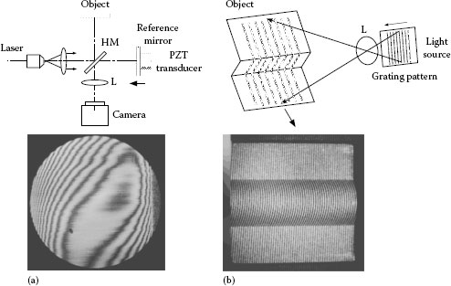
FIGURE 21.1  Examples of fringe images with their formation method: (a) a contour-like interference fringe generated by the Michelson type interferometer, (b) a deformed grating image by a surface shape of an object obtained with the fringe projection method. HM, half mirror; L, imaging lens.

Although the intensity profile of the fringe patterns grabbed in a computer from a CCD camera, for example, is not exactly sinusoidal, the sinusoidal representation is conventional in many cases for mathematical treatments. Thus, in general, an intensity distribution of fringe patterns using sine function is expressed as

$\begin{array}{ll}I\left(x,y\right)\hfill & =I_0\left(x,y\right)\left\{1+\text{γ}\left(x,y\right)\cos \left[\varphi \left(x,y\right)\right]\right\}\hfill \\ \hfill & =a\left(x,y\right)+b\left(x,y\right)\cos \varphi \left(x,y\right),\hfill \end{array}$

(21.1)

where I₀(x, y) and γ(x, y) are the bias intensity and the modulation depth of the fringes in the field of view, which is namely the background intensity distribution and the contrast heterogeneity, and are henceforth substituted as a(x, y) and b(x, y) for simplicity. In many cases, the required value is the phase distribution ϕ(x, y). In the early period of the computer’s introduction, an image processing technique for contour-like fringes, including extractions of the fringe centers and their order number evaluations, was mainstream in the fringe analysis where the sub-fringe order was estimated through the interpolation between fringe centers. The use of this analysis principle is rare nowadays.

Alternatively, more sophisticated analysis principles were evolved after the 1970s; they are, namely, the sub-fringe phase analysis represented by the fringe scanning method [1], the phase-shifting method [2], and the Fourier transformation (FT) method [3]. These methods are classified by the number of input fringe images needed for the phase extraction.

1.  Method using multiple-input images, in which more than three fringe images, whose initial phases are shifted by a given amount (phase-shifted fringes), are acquired and used for the analysis. The phase-shifting method and the fringe-scanning method belong to this class.

2.  Method using single-input image, in which a fringe image introducing the high-frequency carrier fringes is acquired and directly analyzed. The FT method is a typical example.

Next, the principles in each class of the fringe analysis are briefly explained.

21.2.1    METHOD USING MULTIPLE-INPUT IMAGES

The phase-shifting method is the most popular fringe analysis method using multiple-input images. In this method, multiple (N) fringe patterns with the initial phase of a target object shifted by a given value of Δψ are first acquired by some means. These phase-shifted fringe images are obtained at different timings or sampling spaces. In the interferometer as shown in Figure 21.1a, the optical path length of the reference arm is gradually changed by a small displacement of λ × (Δψ)/(2π) (λ is the wavelength of a light source) with a mirror translated by, for example, a PZT transducer. In a grating projection method, the phase shifting is realized by giving in-plane shifts to the grating perpendicularly by a distance of Λ × (Δψ)/(2π) (Λ is the pitch of gratings) as shown in Figure 21.1b.

For the sampling number k = 1, 2, …, N, the phase shift value is usually settled by

$\text{Δ}\psi =\frac{2\pi }{N}.$

(21.2)

For each shifted phase, the N images of fringe intensity distributions,

$I_k\left(x,y\right)=a\left(x,y\right)+b\left(x,y\right)\cos \left[\varphi \left(x,y\right)+\left(k-1\right)\text{Δ}\psi \right],$

(21.3)

are acquired or sampled. By using all the images, the relation between the phase map ϕ(x, y) and the intensity values at each pixel is deduced as their general least square solution:

$\tan \varphi \left(x,y\right)=\frac{{\displaystyle {\sum }_{k=1}^N{I}_k\left(x,y\right)\sin \left[\left(k-1\right)\text{Δ}\psi \right]}}{{\displaystyle {\sum }_{k=1}^N{I}_k\left(x,y\right)\cos \left[\left(k-1\right)\text{Δ}\psi \right]}}.$

(21.4)

In principle, the larger sampling number N decreases the random intensity noise by the factor of $1/\sqrt{N}$ and gives rise to the high accuracy in measurements. In practice, however, from three to seven phase-shifted fringes are used for the analysis. There were various sampling algorithms depending on the number N reported, which are called “N steps” or “N buckets” algorithms [2].

The most basic algorithm corresponds to the case that the sampling number of the phase-shifted fringes is equal to the unknown parameters to be measured, I₀, γ, and ϕ, that is, N = 3, with the phase-shifting of Δψ = π/2. Then, the phase map is retrieved by the following equation:

$\varphi \left(x,y\right)={\tan }^{-1}\left[\frac{I_3\left(x,y\right)-I_2\left(x,y\right)}{I_1\left(x,y\right)-I_2\left(x,y\right)}\right]+\frac{\pi }{4},$

(21.5)

where tan⁻¹ is the arctangent. Furthermore, the contrast map of fringes is also calculated with

$\text{γ}\left(x,y\right)=\frac{\sqrt{{\left[I_1\left(x,y\right)-I_2\left(x,y\right)\right]}^2+{\left[I_2\left(x,y\right)-I_3\left(x,y\right)\right]}^2}}{2I_0},$

(21.6)

and the bias intensity of fringes is estimated by

$I_0\left(x,y\right)=\frac{I_1\left(x,y\right)+I_3\left(x,y\right)}{2}.$

(21.7)

For the most popular algorithm in the case of using the four phase-shifting fringes (four-steps or four-buckets algorithms with N = 4 and Δψ = π/2), the equations shown in Table 21.1 (four-steps method) are normally used.

TABLE 21.1
Frequently Used or Improved Phase-Shifting Algorithms

Four-steps method [2]
Phase shift	Δψ = π/2
Phase map	$\varphi \left(x,y\right)={\tan }^{-1}\frac{I_4\left(x,y\right)-I_2\left(x,y\right)}{I_1\left(x,y\right)-I_3\left(x,y\right)}$
Contrast map	$\text{γ}\left(x,y\right)=\frac{\sqrt[2]{{\left[I_1\left(x,y\right)-I_3\left(x,y\right)\right]}^2+{\left[I_2\left(x,y\right)-I_4\left(x,y\right)\right]}^2}}{I_1\left(x,y\right)+I_2\left(x,y\right)+I_3\left(x,y\right)+I_4\left(x,y\right)}$
Carre’s method (four steps) [4]
Phase shift	Δψ = α (arbitrary constant) Phase shift α is obtained by (coordinates (x, y) are omitted) $\alpha =2{\tan }^{-1}\sqrt{\frac{\left[3\left(I_2-I_3\right)-\left(I_1-I_4\right)\right]}{\left[\left(I_2-I_3\right)+\left(I_1-I_4\right)\right]}}$
Phase map	$\varphi ={\tan }^{-1}\frac{\sqrt{\left[3\left(I_2-I_3\right)-\left(I_1-I_4\right)\right]\left[\left(I_2-I_3\right)+\left(I_1-I_4\right)\right]}}{\left(I_2-I_3\right)-\left(I_1-I_4\right)}$
Contrast map	$\text{γ\hspace{0.17em}}=\frac{1}{2I_0}\sqrt{\frac{{\left[\left(I_2-I_3\right)+\left(I_1-I_4\right)\right]}^2+{\left[\left(I_2+I_3\right)-\left(I_1+I_4\right)\right]}^2}{2}}$
Hariharan’s five-steps method [5]
Phase shift	ψ Δ = π/2
Phase map	$\varphi \left(x,y\right)={\tan }^{-1}\frac{2\left[I_2\left(x,y\right)-I_4\left(x,y\right)\right]}{2I_3\left(x,y\right)-I_5\left(x,y\right)-I_1\left(x,y\right)}$ $\cos \text{Δ}\psi =\frac{I_5-I_1}{2\left(I_4-I_2\right)}\Rightarrow 0$ for calibrations of the phase shift value

Notice that in the use of the above algorithms, since exact and known phase-shifting values are presumed, highly accurate phase shifters should be used and that phase-shifting errors are also introduced by various disturbances such as vibration among image acquisitions and could give rise to serious measurement errors. In particular, linear and nonlinear deviations in phase shifts are mainly caused by calibration error and the drift of the phase shifters such as a PZT, which are major sources for the phase-measurement errors as well as the deviation of fringe profiles from the exact sinusoidal shapes. For these problems, several error-correction algorithms have been proposed.

For example, in the case where the phase-shift value Δψ is deviated from π/2 but is constant, an error-correction method using four phase steps has been proposed by Carré [4], which is shown in Table 21.1 (Carré’s method [four steps]). For the fringe profiles containing spatial nonuniformity such as second order frequency components, a five-steps algorithm shown in Table 21.1 (Hariharan’s five-steps method) is frequently adopted as an error compensation [5]. Various improved algorithms have been proposed against nonlinear phase-shift errors, vibrations at specific frequency, and others [6,7,8].

Figure 21.2 shows a practical procedure of the fringe analysis based on three-buckets phase-shifting method. The optical setup is the Michelson type interferometer, the same as that in Figure 21.1a. The reference mirror was displaced stepwise by π/2 in phase with a PZT transducer and the phase-shifted fringe patterns were stored in a frame grabber as shown in Figure 21.2a. Next, the phase map in Figure 21.2b was derived from the three images through the image operations for each pixel based on Equation 21.5. In the phase map, black (gray level 0) corresponds to −π in phase and white (gray level 255) to +π. To convert the phase map to the actual physical information, for example, maps of the optical path differences or object surface height, an additional operation to the phase map, called “phase unwrapping,” is necessary as described later. Finally, the surface height map of the object is deduced using the physical relation between the phase ϕ and the height Δz, λ × (ϕ/2π) = 2Δz, as shown in Figure 21.2c.

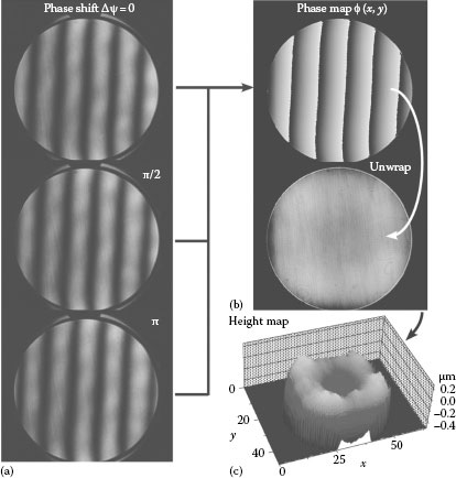
FIGURE 21.2  Fringe analysis procedure in three-buckets phase-shifting method: (a) input fringe patterns with phase shifted by π/2 rad for each, (b) an obtained phase map and its unwrapped results (the detail described after), and (c) a finally obtained height (optical path difference) map.

A merit of the phase-shifting method is the pixel-by-pixel operation for obtaining the phase value to be measured, by which no spatial resolution is sacrificed and the accuracy of phase calculation can be easily improved by increasing the image sampling numbers. On the contrary, because of the necessity for acquiring multiple images at different timings, it is easily influenced by surrounding disturbances like vibrations and is not suitable for an instantaneous measurement of moving objects. To meet such applications, several techniques obtaining the phase-shifted fringes spatially parallel have been proposed, where the multiple phase-shifted fringes are generated, for example, by a parallel polarization interferometer or a grating interferometer, and are simultaneously acquired with single or multiple cameras [9,10,11].

21.2.2    Method using Single-Input Image

As described before, the fringe analysis using multiple fringe patterns needs special equipment introducing the phase shift and usually does not suit dynamic measurements. As a complementary principle, there are proposed fringe analysis methods using a single fringe pattern in which the pattern superposed with equispaced fringes that have higher spatial frequency, namely, carrier fringes, enough for that of the phase gradient to be measured is acquired. The word “carrier fringes” is derived from the concept of a carrier wave used in communication technology and corresponds, for instance, to the dense fringe condition generated by tilting a reference mirror in an interferometer, as shown in Figure 21.3. Here, simply suppose the case introducing the carrier fringes with a spatial frequency of f₀ (1/pixel) along the one-dimensional axis x as in Figure 21.4a. The intensity distribution of this fringe pattern is expressed by

$I\left(x,y\right)=a\left(x,y\right)+b\left(x,y\right)\cos \left[2\pi f_{0}x+\varphi \left(x,y\right)\right],$

(21.8)

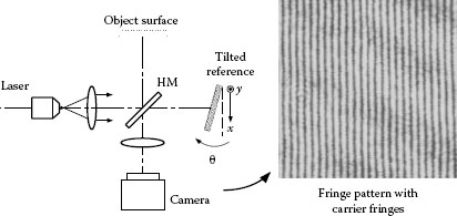
FIGURE 21.3  Introducing way of the carrier fringes in an interferometer and an example of the fringe pattern.

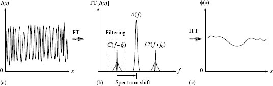
FIGURE 21.4  Signal processing flow in FT method: (a) phase-modulated carrier fringes, (b) filtering and shift in spectrum space, and (c) demodulated phase.

where the phase term ϕ(x, y) deforms the equispaced carrier fringes. This situation can be regarded as a spatial phase modulation of carrier fringes with a fundamental frequency of f₀. Considering this aspect, various phase-demodulation algorithms can be applied. The principal way is the FT method which extracts only the modulated phase term through spectrum filtering, using one- or two-dimensional FT and its inversion [3].

In the case of introducing the carrier fringes in the interferometer as shown in Figure 21.3, the reference mirror is tilted by a small angle of θ about the y-axis to generate carrier fringes with a spatial frequency of f₀ = (2 tan θ)/λ along the x-axis. The fringe intensity distribution expressed by Equation 21.8 can be substituted to the complex form by using a relation c(x, y) = (1/2)b(x, y) exp[iϕ(x, y)] as

$I\left(x,y\right)=a\left(x,y\right)+c\left(x,y\right)\exp \left(2\pi i{f}_{0}x\right)+c^{\ast }\left(x,y\right)\exp \left(-2\pi i{f}_{0}x\right),$

(21.9)

where c* represents a complex conjugate of c. By performing one-dimensional FT in terms of the coordinate x to the above equation, the spatial frequency spectrum along the axis is derived as

$\begin{array}{ll}\text{FT}\left[I\left(x,y\right)\right]\hfill & ={\displaystyle \underset{-\infty }{\overset{\infty }{\int }}I\left(x,y\right)\exp \left(-2\pi ifx\right)\text{d}x}\hfill \\ \hfill & =A\left(f,y\right)+C\left(f-f_0,y\right)+C^{\ast }\left(f+f_0,y\right),\hfill \end{array}$

(21.10)

where A(f, y) and C(f, y) correspond to the Fourier transforms of a(x, y) and c(x, y), respectively. As known from Figure 21.4b, if we select the larger enough carrier frequency f₀ than that of spatial variations of a(x, y) and b(x, y), the above major spectrums A, C, and C* can be easily separated. Consequently, by applying a sequential processing, which consists of the extraction of the C(f – f₀, y) component with a window filtering, its spectrum shift to the zero frequency position, and the inverse FT of the modified signal, the carrier frequency components are removed and only the desired component c(x, y) is demodulated. Finally, in Figure 21.4c, the phase distribution ϕ(x, y) is calculated by taking log c(x, y) or using the arctangential relation for the real and imaginary parts of c(x, y):

$\varphi \left(x,y\right)={\tan }^{-1}\frac{\mathrm{Im}\left[c\left(x,y\right)\right]}{\mathrm{Re}\left[c\left(x,y\right)\right]}.$

(21.11)

The procedure shown in Figure 21.4 can easily be extended to the two-dimensional (2D) FT and filtering in a 2D frequency space, which can be used for the 2D analysis of the fringe pattern superposed with obliquely introduced carrier fringes. An example of phase-extraction procedures for this case is shown in Figure 21.5a through c.

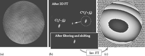
FIGURE 21.5  Phase map extraction in 2D FT method: (a) input fringe patterns with oblique carrier fringes introduced, (b) an FT result of the input pattern is filtered around carrier frequency and shifted to zero frequency position in 2D spectrum space, and (c) a finally extracted phase map obtained after an inverse 2D FT.

Figure 21.5a is an interferogram obtained by a Fizeau interferometer with slight tilts of the reference mirror around both x- and y-axes in which oblique dense carrier fringes are introduced. After the 2D FT for the input fringes, the 2D spectrum distribution shown in the upper frame in Figure 21.5b is obtained, where the two symmetrical spectrum peaks for the modulated carrier fringes terms, C*(f ± f₀), are clearly separated from the peak for the bias terms located at the central zero frequency position. By cutting out one of the carried spectrum peaks, for example, in a circular window (dotted circle in the figure) and shifting to the center, the lower figure in Figure 21.5b is prepared and is again processed with the inverse 2D FT to generate the phase distribution of the object wavefront according to Equation 21.11. Since the fringe intensity profile in the Fizeau interferometer is usually largely deviated from a sinusoidal shape because of multiple reflections, the phase-shifting method described in the last section. On the contrary, this FT method provides accurate results for this case. In the actual processing with computers in the above analysis, the fast FT, whose processing performances have recently become better thanks to the speeding up of the computers and the developments of the speedy and efficient calculation algorithms [12], is usually applied.

The fringe analysis using a single fringe pattern can be performed by the simple or basic optical setup of interferometers or grating projectors and does not require special instruments such as phase shifters. Its one shot measurement capability is suitable for dynamic objects and phenomena. It should be noted that the spatial resolution in this method is variable dependent on the size of the spectrum filtering windows and that aberrations of the used imaging optics and the border of the sampling area cause considerably more phase errors than the former methods using multiple fringe images. As the other phase demodulation methods use a single-input fringe pattern, a variety of techniques, such as the synchronous detection or spatial phase synchronization methods [13,14,15], the phase-locked loop method [16,17], and the spatial phase-shifting or the electronic Moiré methods, have been proposed mainly for the suppression of the processing time or their implements on hardware [18,19,20].

The readers are referred to the other literature for a detailed comparison of the principles and accuracies of the two classes of fringe analysis mentioned here [21].

21.3    PHASE UNWRAPPING

In the usual fringe analysis since the fringe order cannot usually be decided a priori, only the fractional phase divided by 2π is “wrapped” in the region between −π and +π. This leads to discontinuous phase jumps between adjacent pixels from +π to -π or its opposite direction. Therefore, the procedure to connect the discontinuous phase jumps, assuming the spatial continuity of the phase distribution, becomes necessary for obtaining the final physical distribution, as shown in Figure 21.6. This procedure is called as “phase unwrapping.”

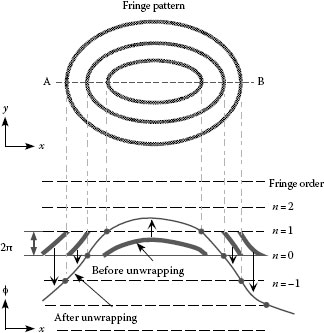
FIGURE 21.6  Concept of the phase unwrapping in the fringe analysis.

In most simple cases of phase unwrapping, the phase differences between adjacent pixels along the one-dimensional unwrapping path are estimated and are connected by using the following operations:

$\begin{array}{ll}\text{If}\hfill & \varphi \left(r_{i+1}\right)-\varphi \left(r_i\right)>\pi \hfill \\ \hfill & \varphi \left(r_{i+1}\right)=\varphi \left(r_{i+1}\right)-2\pi \hfill \\ \text{else},\text{if}\hfill & \varphi \left(r_{i+1}\right)-\varphi \left(r_i\right)\le -\pi \hfill \\ \hfill & \varphi \left(r_{i+1}\right)=\varphi \left(r_{i+1}\right)+2\pi ,\hfill \end{array}$

(21.12)

where r_i is the vectorial position at pixel number i. If the effective phase area is a rectangular x – y coordinate, a combination of unwrappings on all horizontal paths along x-axis and one along the vertical y-axis gives an appropriate result [22]. However, general fringe patterns to be measured might be surrounded by a nonrectangle boundary and might contain pixels considered as singular points, where the fringe modulation is very low or the actual phase differences are larger than 2π against some of the adjacent pixels. In these situations, the above phase-unwrapping path is accidentally interrupted and the unwrapped phase distribution is deviated from the true one. However, several effective and robust phase-unwrapping algorithms have been proposed to avoid these problems as follows:

1.  Algorithms based on the minimum-spanning tree tracking: Methods to obtain a continuous phase-unwrapping path by spanning the effective phase area with tree-like trajectories that have no localized closed loop. To select the effective path, cost functions such as the spatial phase gradient and the fringe contrast are used to decide the reliability of the pixels. Unreliable pixels are removed from the spanning tree. Highspeed algorithms [23,24].

2.  Algorithms based on energy minimization: Methods to realize the optimum unwrapped state by minimizing the energy function, based on the summation of the phase differences among the neighboring pixels in which the initial phase distribution corresponds to the maximum energy state, are converged to the minimum energy state by varying the phases at all pixels by ±2π based on a certain rule. This method requires many steps of iteration for convergence and does not depend on the unwrapping path. There are several algorithms proposed such as the simulated annealing method [25], a method using the Euler–Poisson equation [26], and the cellular automata method [27,28].

In the above procedure, the singular points mentioned earlier should be checked in advance and removed from the unwrapping operations. To check the singularity of the pixels, the rotating phase-unwrapping operation for the local four neighboring pixels (Figure 21.7) is frequently applied. In some cases, a line joining two singular points having different signs (right-handed or left-handed) can be used as a cutline for the phase-unwrapping path finding. A method to directly remove singular points from a phase distribution has also been proposed [29].

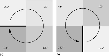
FIGURE 21.7  Singular points generated for four neighboring pixels in phase-unwrapping procedure. (a) Right-handed singular point with abnormal phase jump along horizontal left direction. (b) Left-handed singular point with abnormal phase jump along vertical down direction.

21.4    PRACTICAL EXAMPLE OF FRINGE ANALYSIS IN PROFILOMETRY

Finally, we show an actual process of the fringe analysis for profilometry using the deformed grating method with an interference fringe projection. The obliquely projected equispaced fringes on the object are deformed and phase modulated depending on the surface profile by being observed from a different direction. Modulated phases have to be extracted from a single fringe pattern. The overall processing flow of the fringe analysis is shown in Figure 21.8a through f. The image in Figure 21.8a is the input fringe pattern where the carrier-introduced interference fringes are projected on a face of a “Hina” doll and the deformed fringes on the face profile are captured by a CCD camera to be stored as a digitized image of 8 bits grayscale in a frame grabber of 512 × 512 pixels. Here, care should be taken in the matching of the fringe’s modulation depth to the digitizing range of the frame grabber through the tuning or exposure condition.

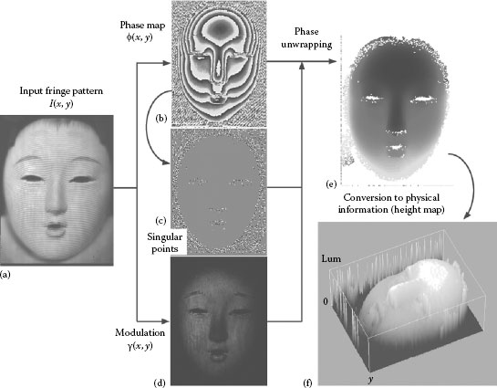
FIGURE 21.8  Practical processing flow of fringe analysis in the case of the profile measurement by the deformed grating method with an interference fringe projection. (a) Input image obtained from a face of a “Hina” doll under the projection of carrier fringe pattern, (b) phase map extracted with the electronic Moiré technique, (c) singular points map extracted from the phase map, (d) modulation depth map of the fringe pattern, (e) processing result after the phase unwrapping based on the minimum spanning tree method with the removal of unreliable pixels in terms of the singularity and the modulation depth, and (f) finally obtained profile of the target surface.

The electronic Moiré technique [21] was used as the fringe analysis method, in which three phase-shifted Moiré fringes are digitally generated in a computer by multiplying the input fringes to three phase-shifted reference fringes prepared in the memory and spatially low-pass filtering them. The distributions of the phase and the modulation depth shown in Figure 21.8b and c are calculated using Equations 21.5 and 21.6 with three Moiré fringes. As the pretreatment before the phase unwrapping, the map of the singular points in Figure 21.8d is extracted from the wrapped phase map as described in the previous section. White- and black-colored pixels in Figure 21.8d correspond to the extracted singular points with different signs. The modulation depth information is also used to remove the pixels with low modulation depth from the phase-unwrapping operation. By using the information on singular points and the modulation depth as the cost function, the phase map in Figure 21.8b is phase unwrapped with the minimum spanning tree method to generate a smooth unwrapped phase, as shown in Figure 21.8e. Finally, the obtained unwrapped phase map is converted to the physical height map of the object surface by taking into account various parameters in the deformation grating method such as the projected fringe pitch, projection angle, and the imaging conditions including the calibration factor [30]. Figure 21.8f shows the 3D representation of the finally measured surface profile of the object.

21.5    SUMMARY

In this chapter, the basic principles and concepts of the generally used fringe analysis are briefly explained. Nowadays, fringe analysis is widely used in many fields where a variety of novel techniques including spatiotemporal modulation of the various parameters like fringe pitch, frequency, and fringe orientation are being developed. Recent rapid evolution of computers, imaging devices, and light sources must further expand the application fields of fringe analysis.

SYMBOLS

I	Fringe intensity
x, y	Coordinates
I0, γ	Bias intensity and modulation depth of fringes
a, b	Background intensity and contrast of fringes
ϕ	Phase term of fringe pattern
λ	Wavelength of light
Λ	Pitch of projection grating
Δψ	Phase-shifting value
N	Number of frames used in phase-shifting method
k	Sampling number of phase-shifted fringes
Ik	Fringe intensity kth sample
α	Constant but unknown phase-shifting value
Δz	Object height
f, f0	Frequencies of original fringe and carrier fringes
θ	Tilting angle
c, C	Complex amplitude and its Fourier transform
r	Vectorial position

REFERENCES

1.  Bruning, J. H., Herriott, D. R., Callagher, J. E., Rosenfeld, D. P., White, A. D., and Brangaccio, D. J. 1974. Digital wavefront measuring interferometer for testing optical surfaces and lenses. Appl. Opt. 13:2693–2703.

2.  Creath, K. 1988. Phase-measurement interferometry techniques. In Progress in Optics XXVI, E. Wolf (Ed.), pp. 349–393, Amsterdam, the Netherlands: Elsevier.

3.  Takeda, M., Ina, H., and Kobayashi, S. 1982. Fourier-transform method of fringe-pattern analysis for computer-based topography and interferometry. J. Opt. Soc. Am. 72:156–160.

4.  Carré, P. 1966. Installation et utilisation du comparateur photoelectrique et interferentiel du Bureau International des Poids et Mesures. Metrologia 2:13–23.

5.  Hariharan, P., Oreb, B. F., and Eiju, T. 1987. Digital phase-shifting interferometry: A simple error-compensating phase calculation algorithm. Appl. Opt. 26:2504–2506.

6.  Hibino, K., Oreb, B. F., Farrant, D. I., and Larkin, K. G. 1997. Phase-shifting algorithms for nonlinear and spatially nonuniform phase shifts. J. Opt. Soc. Am. A 14:918–930.

7.  de Groot, P. J. 1995. Vibration in phase-shifting interferometry. J. Opt. Soc. Am. A 12:354–365.

8.  Zhu, Y.-C. and Gemma, T. 2001. Method for designing error-compensating phase-calculation algorithms for phase-shifting interferometry. Appl. Opt. 40:4540–4546.

9.  Onuma, K., Tsukamoto, K., and Nakadate, S. 1993. Application of real-time phase-shift interferometer to the measurement of concentration field. J. Crystal Growth 129:706–718.

10.  Kwon, O. Y. 1984. Multichannel phase-shifted interferometer. Opt. Lett. 9:59–61.

11.  Qian, K., Wu, X.-P., and Asundi, A. 2002. Grating-based real-time polarization phase-shifting interferometry: Error analysis. Appl. Opt. 41:2448–2453.

12.  http://www.fftw.org/.

13.  Ichioka, Y. and Inuiya, M. 1972. Direct phase detecting system. Appl. Opt. 11:1507–1514.

14.  Womack, K. H. 1984. Interferometric phase measurement using spatial synchronous detection. Opt. Eng. 23:391–395.

15.  Toyooka, S. and Tominaga, M. 1984. Spatial fringe scanning for optical phase measurement. Opt. Commun. 51:68–70.

16.  Kato, J., Tanaka, T., Ozono, S., Fujita, K., Shizawa, M., and Takamasu, K. 1988. Real-time phase detection for fringe-pattern analysis using digital signal processing. Proc. SPIE 1032:791–796; Kato, J. et al. 1993. A real-time profile restoration method from fringe patterns using digital phase-locked loop—Improvement of the accuracy and its application to profile measurement of optical surface. Jpn. J. Prec. Eng. 59:1549–1554 (in Japanese).

17.  Servin, M. and Rodriguez-Vera, R. 1993. Two-dimensional phase locked loop demodulation of interferograms. J. Mod. Opt. 40:2087–2094.

18.  Williams, D. C., Nassar, N. S., Banyard, J. E., and Virdee, M. S. 1991. Digital phase-step interferometry: A simplified approach. Opt. Laser Technol. 23:147–150.

19.  Küchel, M. 1990. The new Zeiss interferometer. Proc. SPIE 1332:655–663.

20.  Kato, J., Yamaguchi, I., Nakamura, T., and Kuwashima, S. 1997. Video-rate fringe analyzer based on phase-shifting electronic Moiré patterns. Appl. Opt. 36:8403–8412.

21.  Takeda, M. 1984. Subfringe interferometry fundamentals, KOGAKU 13:55 (in Japanese).

22.  Itoh, K. 1982. Analysis of the phase unwrapping algorithm. Appl. Opt. 21:2470.

23.  Judge, T. R., Quan, C.-G., and Bryanstoncross, P. J. 1992. Holographic deformation measurements by Fourier-transform technique with automatic phase unwrapping. Opt. Eng. 31:533–543.

24.  Takeda, M. and Abe, T. 1996. Phase unwrapping by a maximum cross-amplitude spanning tree algorithm: A comparative study. Opt. Eng. 35:2345–2351.

25.  Huntley, J. M. 1989. Noise-immune phase unwrapping algorithm. Appl. Opt. 28:3268–3270.

26.  Kerr, D., Kaufmann, G. H., and Galizzi, G. E. 1996. Unwrapping of interferometric phase-fringe maps by the discrete cosine transform. Appl. Opt. 35:810–816.

27.  Ghiglia, D. C., Mastin, G. A., and Romero, L. A. 1987. Cellular-automata method for phase unwrapping. J. Opt. Soc. Am. A 4:267–180.

28.  Ghiglia, D. C. and Pritt, M. D. 1998. Two-Dimensional Phase Unwrapping: Theory, Algorithms, and Software. New York: Wiley-Interscience.

29.  Aoki, T., Sotomaru, T., Ozawa, T., Komiyama, T., Miyamoto, Y., and Takeda, M. 1998. Opt. Rev. 5:374–379.

30.  Sansoni, G., Carocci, M., and Rodella, R. 1999. Three-dimensional vision based on a combination of gray-code and phase-shift light projection: Analysis and compensation of the systematic errors. Appl. Opt. 38:6565–6573 (For example).