Chapter 1 Light Sources

This chapter offers a review of radiometry, photometry, and light sources in terms of the basic notions and principles of measurement of electromagnetic radiation that are most relevant for optical metrology. It explains the difference between radiometry and photometry, and their quantities and units. More information on these topics can be found in specialized literature (e.g., see Refs. [1,2,3,4,5,6,7,8]). This chapter also includes a brief survey of conventional light sources. Special attention is paid to modern light sources such as lasers, light emitting diodes (LEDs), and super luminescent diodes (SLDs), which are widely used in the contemporary techniques of optical metrology. There is an enormous amount of literature on this topic, but the reader may want to start with the detailed reviews of LED that are given in some introductory books (e.g., Refs. [9,10,11,12] and references therein).

1.1 RADIOMETRY AND PHOTOMETRY

1.1.1 DIFFERENCES BETWEEN RADIOMETRY AND PHOTOMETRY

Radiometry is the science of measurement of electromagnetic radiation within the entire range of optical frequencies between 3 × 10¹¹ and 3 × 10¹⁶ Hz, which corresponds to wavelengths between 0.01 and 1000 μm. The optical range includes the ultraviolet (UV), the visible, and the infrared (IR) regions of the electromagnetic spectrum. Radiometry explores the electromagnetic radiation as it is emitted and detected, and measures quantities in terms of absolute power as measured with a photodetector. It considers the related quantities such as energy and power, as independent of wavelength. The relevant quantities are designated as radiant and their units are derivatives of joules.

Photometry deals with the part of the electromagnetic spectrum that is detectable by the human eye, and therefore, it is restricted to the frequency range from about 3.61 × 10¹⁴ to roughly 8.33 × 10¹⁴ Hz (which is the wavelength range from about 830 to 360 nm). These limits of the visible part of the spectrum are specified by the International Commission on Illumination (CIE; Commission Internationale de l’Éclairage). The emission of light results from rearrangement of the outer electrons in atoms and molecules, which explains the very narrow band of frequencies in the spectrum of electromagnetic radiation corresponding to light. Photometry is the science of measurement of light, in terms of its perceived brightness to the human eye; thus, it measures the visual response. Therefore, photometry considers the wavelength dependence of the quantities associated with radiant energy and new units are introduced for the radiometric quantities. The photometric quantities are designated as luminous. Typical photometric units are lumen, lux, and candela.

When the eye is used as a comparison detector, we speak about visual photometry. Physical photometry uses either optical radiation detectors that mimic the spectral response of the human eye or radiometric measurements of a radiant quantity (i.e., radiant power), which is later weighted at each wavelength by the luminosity function that models the eye brightness sensitivity. Photometry is a basic method in astronomy, as well as in lighting industry, where the properties of human vision determine the quantity and quality requirements for lighting.

Colorimetry is the science and measurements of color. The fundamentals of colorimetry are well presented, for example, in Refs. [13,14].

1.1.2 HUMAN EYE

The human eye is not equally sensitive to all the wavelengths of light. The eye is most sensitive to green–yellow light, the wavelength range where the sun has its peak energy density emission, and the eye sensitivity curve falls off at higher and lower wavelengths. The eye response to light and color depends also on light conditions and is determined by the anatomical construction of the human eye, described in detail in Encyclopedia Britannica, 1994. The retina includes rod and cone light receptors. Cone cells are responsible for the color perception of the eye and define the light-adapted vision, that is, the photopic vision. The cones exhibit high resolution in the central part of the retina, the foveal region (fovea centralis), which is the region of greatest visual acuity. There are three types of cone cells, which are sensitive to red, green, and blue light. The second type of cells, the rods, are more sensitive to light than cone cells. In addition, they are sensitive over the entire visible range and play an important role in night vision. They define the scotopic vision, which is the human vision at low luminance. They have lower resolution ability than the foveal cones. Rods are located outside the foveal region, and therefore, are responsible for the peripheral vision. The response of the rods at high-ambient-light levels is saturated and the vision is determined entirely by the cone cells (see also Refs. [5,15]). Photometry is based on the eye’s photopic response, and therefore, photometric measurements will not accurately indicate the perceived brightness of sources in dim lighting conditions.

The sensitivity of eye to light of different wavelength is given in Figure 1.1. The light-adapted relative spectral response of the eye is called the spectral luminous efficiency function for photopic vision, V(λ). The dark-adapted relative spectral response of the eye is called the spectral luminous efficiency function for scotopic vision, V′(λ). Both are empirical curves. The curve of photopic vision, V(λ), was first adopted by CIE in 1924. It has a peak of unity at 555 nm in air (in the yellow–green region), reaches 50% at near 510 and 610 nm and decreases to levels below 10⁻⁵ at about 380 and 780 nm. The curve for scotopic vision, V′(λ), was adopted by the CIE in 1951. The maximum of the scotopic spectrum is shifted to smaller wavelengths with respect to the photopic spectrum. The V′(λ) curve has a peak of unity at 507 nm, reaches 50% at about 455 and 550 nm, and decreases to levels below 10⁻³ at about 380 and 645 nm. Photopic or light-adapted cone vision is active for luminances greater than 3 cd/m². Scotopic or dark-adapted rod vision is active for luminances lower than 0.01 cd/m². The vision in the range between these values is called mesopic and is a result of varying amounts of contribution of both rods and cones.

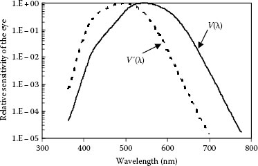
FIGURE 1.1 Spectral sensitivity of the human eye. The solid line is the curve V(λ) for photopic vision from 1924 CIE, and the dashed line is the curve for scotopic vision V′(λ) from 1951 CIE. (Žukauskas, A., Shur, M.S., and Gaska, R.: Introduction to Solid-State Lighting. 2002. Copyright Wiley-VCH Verlag GmbH & Co. KGaA. Reproduced with permission.)

As most of the human activities are at high-ambient illumination, the spectral response and color resolution of photopic vision have been extensively studied. Recent measurements of the eye response to light have made incremental improvement of the initial CIE curves, which underestimated the response at wavelengths shorter than 460 nm [16,17,18,19,20]. The curves V(λ) and V′(λ) can easily be fit with a Gaussian function by using a nonlinear regression technique, as the best fits are obtained with the following equations [21]:

$\begin{array}{l} V (λ) ≅ 1.019 e^{- 285.4 {(λ - 0.559)}^{2}} for photopic vision \\ V^{'} (λ) ≅ 0.992 e^{- 321.9 {(λ - 0.503)}^{2}} for phtopic vision \end{array}$ $\begin{array}{l} V (λ) ≅ 1.019 e^{- 285.4 {(λ - 0.559)}^{2}} for photopic vision \\ V^{'} (λ) ≅ 0.992 e^{- 321.9 {(λ - 0.503)}^{2}} for phtopic vision \end{array}$

However, the fit of the scotopic curve is not quite good as the photopic curve. The Gaussian fit with the functions above is only an approximation that is acceptable for smooth curves but is not appropriate for narrow wavelength sources, like LEDs.

1.1.3 RADIOMETRIC AND PHOTOMETRIC QUANTITIES AND UNITS

Radiometric quantities characterize the energy content of radiation, whereas photometric quantities characterize the response of the human eye to light and color. Therefore, different names and units are used for photometric quantities. Every quantity in one system has an analogous quantity in the other system. Many radiometric and photometric terms and units have been used in the optics literature; however, we will consider here only the SI units.

A summary of the most important photometric quantities and units with their radiometric counterparts are given in Table 1.1. Radiometric quantities appear in the literature either without subscripts or with the subscript e (electromagnetic). Photometric quantities usually are labeled with a subscript λ or v (visible) to indicate that only the visible spectrum is being considered. In our text, we use the subscript λ for the symbols of photometric quantities and no subscript for the radiometric quantities. Subsequently, we define in more detail the terms in Table 1.1 and their units.

TABLE 1.1
Radiometric and Photometric Quantities and Units

	Radiometric Quantities	Units	Photometric Quantities	Units
Energy	Radiant energy Q	J (joule)	Luminous energy Q_λ	lm · s (or talbot)
Energy density	Radiant energy density $w = \frac{d Q}{d V}$ $w = \frac{d Q}{d V}$	$\frac{J}{m^{3}}$ $\frac{J}{m^{3}}$	Luminous density $w_{λ} = \frac{d Q_{λ}}{d V}$ $w_{λ} = \frac{d Q_{λ}}{d V}$	$\frac{lm \cdot s}{m^{3}}$ $\frac{lm \cdot s}{m^{3}}$
Power	Radiant flux or radiant power $Φ = \frac{d Q}{d t}$ $Φ = \frac{d Q}{d t}$	W or $\frac{J}{s}$ $\frac{J}{s}$	Luminous flux $Φ_{λ} = \frac{d Q}{d t} λ$ $Φ_{λ} = \frac{d Q}{d t} λ$	lm = cd sr
Power per area	Radiant exitance $M = \frac{d Φ}{d a}$ $M = \frac{d Φ}{d a}$ (for emitter) or irradiance $E = \frac{d Φ}{d a}$ $E = \frac{d Φ}{d a}$ (for receiver)	$\frac{W}{m^{2}}$ $\frac{W}{m^{2}}$	Luminous exitance $M_{λ} = \frac{d Φ_{λ}}{d a}$ $M_{λ} = \frac{d Φ_{λ}}{d a}$ (light emitter) or illuminance (light receiver) $E_{λ} = \frac{d Φ_{λ}}{d a}$ $E_{λ} = \frac{d Φ_{λ}}{d a}$	Lux or $\frac{lm}{m^{2}}$ $\frac{lm}{m^{2}}$
Power per area per solid angle	Radiance $L = \frac{d Φ}{d Ω d a cos α} = \frac{d I}{d a \cos α}$ $L = \frac{d Φ}{d Ω d a cos α} = \frac{d I}{d a \cos α}$	$\frac{W}{sr \cdot m^{2}}$ $\frac{W}{sr \cdot m^{2}}$	Luminance $L_{λ} = \frac{d I_{λ}}{d a \cos α}$ $L_{λ} = \frac{d I_{λ}}{d a \cos α}$	$\frac{cd}{m^{2}} = \frac{lm}{m^{2} \cdot sr}$ $\frac{cd}{m^{2}} = \frac{lm}{m^{2} \cdot sr}$ (or nit)
Intensity	Radiant intensity $I = \frac{d Φ}{d Ω}$ $I = \frac{d Φ}{d Ω}$	$\frac{W}{sr}$ $\frac{W}{sr}$	Luminous intensity $I_{λ} = \frac{d Φ}{d Ω}$ $I_{λ} = \frac{d Φ}{d Ω}$	Candela or $\frac{lm}{sr}$ $\frac{lm}{sr}$

1.1.3.1 Radiometric Quantities and Units

Most of the theoretical models build on the supposition of a point light source that emits in all directions, we have to define first the term “solid angle,” which is measured in steradians (sr). According to NIST SP811, the steradian is defined as follows: “One steradian (sr) is the solid angle that, having its vertex in the center of a sphere, cuts off an area on the surface of the sphere equal to that of a square with sides of length equal to the radius of the sphere.” The solid angle is thus the ratio of the spherical area to the square of the radius. The spherical area is a projection of the object of interest onto a unit sphere, and the solid angle is the surface area of that projection. If we divide the surface area of a sphere by the square of its radius, we find that there are 4π sr of solid angle in a sphere. One hemisphere has 2π sr. The solid angle, as illustrated in Figure 1.2, is defined by the area the cone cuts out from a sphere of radius R = 1 (Figure 1.2). For small solid angles, the spherical section can be approximated with a flat section, and the solid angle is

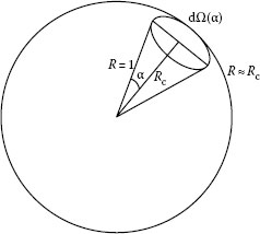
FIGURE 1.2 Definition of solid angle. For a small solid angle, the spherical elemental section is approximated by a flat section and R ≈ R_c.

$d Ω (α) = \frac{π {(R sin α)}^{2}}{R^{2}} = π \sin^{2} α$ $d Ω (α) = \frac{π {(R sin α)}^{2}}{R^{2}} = π \sin^{2} α$

(1.1)

Radiant energy, Q, measured in joules (J) and radiant energy density, w (J/m³), are basic terms that need no further explanation. Radiant flux or radiant power, Φ, is the time rate of flow of radiant energy measured in watts (W = J/s). The radiant energy can be either emitted, scattered, or reflected from a surface (the case of an emitter), or incident onto a surface (the case of a receiver). Thus, different symbols and names may be used for the same quantity for the cases of emitter and receiver.

Radiant intensity, I, is defined as the radiant flux emitted by a point source per unit solid angle, Ω, in a given direction:

$I = \frac{d Φ}{d Ω}$ $I = \frac{d Φ}{d Ω}$

(1.2)

It is expressed in watts per steradian (W/sr). For example, the intensity from a sphere emitting radian flux Φ (W) uniformly in all directions is Φ/4π (W/sr).

In general, the direction of propagation of radiant energy is given by the Poynting vector. The radiant flux density (W/m²) emitted from a surface with a surface area da is called radiant exitance, M,

$M = \frac{d Φ}{d a} [\frac{W}{m^{2}}]$ $M = \frac{d Φ}{d a} [\frac{W}{m^{2}}]$

(1.3a)

The radiant flux density of radiation incident onto a surface with a given area da′ is called irradiance, E. Thus, the irradiance is defined as the radiant flux incident onto a unit area perpendicular to the Poynting vector

$E = \frac{d Φ}{d a^{'}} [\frac{W}{m^{2}}]$ $E = \frac{d Φ}{d a^{'}} [\frac{W}{m^{2}}]$

(1.3b)

For an emitter with a given area and a constant radiant flux, the irradiance is constant. For example, the irradiance of the Sun is E = 1.37 × 10³ W/m². This numerical value is called the solar constant. It describes the solar radiation at normal incidence on an area above the atmosphere. In space, the solar radiation is practically constant, while on Earth it varies with the time of day and year as well as with the latitude and weather. The maximum value on the Earth is between 0.8 and 1.0 kW/m².

Radiant efficiency describes the ability of the source to convert the consumed electric power (IV) into radiant flux Φ:

$Radiant efficiency = Φ / (I V)$ $Radiant efficiency = Φ / (I V)$

(1.4)

Here I and V are the electric current through and potential difference across the light source, respectively. The radiant efficiency is dimensionless and may range from 0 to 1.

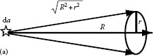
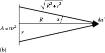
Figure 1.3 represents an emitter with a flat circular area for which the diameter is small compared to the distance R to the receiver. If the area of the emitter is da and a cone of light emerges from each point of this area, the opening of the cone is determined by the area of the receiver da′ (solid lines). The solid angle of the cone, dΩ(α), is given as

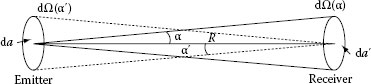
FIGURE 1.3 Opening of the cone toward the receiver determined by the solid angle dΩ(α) = da′/R² and the opening of the cone toward the emitter determined by the solid angle dΩ(α′) = da/R².

$d Ω (α) = \frac{d a^{'}}{R^{2}}$ $d Ω (α) = \frac{d a^{'}}{R^{2}}$

(1.5)

where

α is the half angle of the cross section

da′ is the area of the receiver

Each point of this area receives a cone of light, and the opening of this cone is determined by the area of the emitter da (the cone with dashed lines in Figure 1.3). The solid angle of the cone, dΩ(α′), is given as

$d Ω (α^{'}) = \frac{d a}{R^{2}}$ $d Ω (α^{'}) = \frac{d a}{R^{2}}$

(1.6)

where

α′ is the half angle of the cross section

da is the emitter’s area

The solid angles dΩ(α) and dΩ(α′) illustrate the cone under which the emitter sees the receiver and the receiver sees the emitter.

The radiant flux arriving at the receiver is proportional to the solid angle and the area of the emitter

$Φ - L d a d Ω (α) = L d a \frac{d a^{'}}{R^{2}} [W]$ $Φ - L d a d Ω (α) = L d a \frac{d a^{'}}{R^{2}} [W]$

(1.7)

The constant of proportionality L is called radiance and is equal to the radiant flux arriving at the receiver per unit solid angle and per unit projected source area:

$L = \frac{Φ}{d a d Ω (α)} [\frac{W}{m^{2} \cdot sr}]$ $L = \frac{Φ}{d a d Ω (α)} [\frac{W}{m^{2} \cdot sr}]$

(1.8)

Radiance and irradiance are often confusingly called intensity.

If both the emitter and receiver areas are small compared to their distance from one another, and in addition, if they are perpendicular to the connecting line, Equations 1.1 and 1.7 can be combined to express the radiant flux as

$Φ = L (π {sin}^{2} α) d a$ $Φ = L (π {sin}^{2} α) d a$

(1.9)

The radiant flux from the emitter arriving at the receiver may also be expressed as

$Φ = L d a d Ω (α) = L d a \frac{d a^{'}}{R^{2}} = L d a^{'} \frac{d a^{'}}{R^{2}} = L d a^{'} d Ω (α^{'}) = Φ^{'}$ $Φ = L d a d Ω (α) = L d a \frac{d a^{'}}{R^{2}} = L d a^{'} \frac{d a^{'}}{R^{2}} = L d a^{'} d Ω (α^{'}) = Φ^{'}$

(1.10)

The left side represents the power proportional to the area da of the emitter multiplied by the solid angle dΩ(α), while the right side gives the power proportional to the area da′ of the receiver multiplied by the solid angle dΩ(α′). Both sides should be equal if there are no energy losses in the medium between the emitter and the receiver.

The power arriving at the receiver with area da′ can be expressed by using Equations 1.3 and 1.10 as

$Φ = E d a^{'} = L d a^{'} d Ω (α^{'})$ $Φ = E d a^{'} = L d a^{'} d Ω (α^{'})$

(1.11)

Equation 1.11 gives the relation between irradiance and radiance:

$E = L d Ω (α^{'})$ $E = L d Ω (α^{'})$

(1.12)

The radiance L (W/m²·sr) multiplied by the solid angle results in the irradiance E. The radiance L of Sun can be calculated using Equation 1.12 if we consider Sun as a small, flat emitter and if we bear in mind that Sun is seen from Earth under an angle α = 0.25 ° = 0.004 rad. For a small angle, sin α ≅ α and we can write

$d Ω (α) = π {sin}^{2} (0.25 °) = π {(0.004 rad)}^{2} = 6 \times 10^{- 5} sr$ $d Ω (α) = π {sin}^{2} (0.25 °) = π {(0.004 rad)}^{2} = 6 \times 10^{- 5} sr$

and

$L = \frac{E}{d Ω} = \frac{1.35 \times 10^{3} {W/m}^{2}}{6 \times 10^{- 5} sr} = 2.25 \times 10^{7} \frac{W}{m^{2} \cdot sr}$ $L = \frac{E}{d Ω} = \frac{1.35 \times 10^{3} {W/m}^{2}}{6 \times 10^{- 5} sr} = 2.25 \times 10^{7} \frac{W}{m^{2} \cdot sr}$

Thus, the radiance L of Sun is constant and has the value of 2.25 × 10⁷ W/m²· sr.

1.1.3.2 Lambert’s Law and Lambertian Sources

When we consider an emitter or a receiver, we often refer to them as isotropic and Lambertian surfaces. These two terms are often confused and used interchangeably because both terms involve the implication of the same energy in all directions.

Isotropic surface means a spherical source that radiates the same energy in all directions, that is, the intensity (W/sr) is the same in all directions. A distant star can be considered as an isotropic point source, although an isotropic point source is an idealization and would mean that its energy density would have to be infinite. A small, uniform sphere, such as a globular tungsten lamp with a milky white diffuse envelope, is another good example for an isotropic surface.

Lambertian surface refers to a flat radiating surface, which can be an active surface or a passive, reflective surface. According to Lambert’s law, the intensity for a Lambertian surface falls off as the cosine of the observation angle with respect to the surface normal and the radiance (W/m²·sr) is independent of direction. An example could be a surface painted with a good matte white paint. If it is uniformly illuminated, like from Sun, it appears equally bright from whatever direction you view it. Note that the flat radiating surface can be an elemental area of a curved surface.

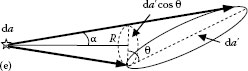
Lambert’s law defines the distribution of the emitted power when the area of the emitter and the receiver are tilted with respect to each other, as shown in Figure 1.4. Let us assume that the emitter and the receiver have small areas da and da′, respectively. The area da is tilted through the angle θ with respect to the line connecting the areas da and da′. In 1769, Johann Lambert found experimentally that when one of both, the emitter or the detector, is tilted through an angle θ with respect to the other, the emitted power depends on θ via cos θ factor. Therefore, this law is known as cosine law of Lambert. The mathematical representation of Lambert’s law is

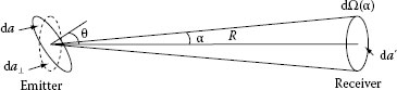
FIGURE 1.4 Illustration of Lambert’s law application. The emitter is tilted in respect with the receiver.

$Φ (θ) = L \frac{d a^{'}}{R^{2}} d a \cos θ = L \frac{d a^{'}}{R^{2}} d a_{⊥}$ $Φ (θ) = L \frac{d a^{'}}{R^{2}} d a \cos θ = L \frac{d a^{'}}{R^{2}} d a_{⊥}$

(1.13)

where da_⊥ = da cos θ is the projection of the area da on the plane perpendicular to the connecting line between emitter and receiver. According to Lambert’s law, the area da, when looked at the angle θ, has the same radiance L as the smaller area da⊥.

If we consider Sun as a sphere consisting of small areas da emitting power Φ(θ) into a solid angle dΩ(α) = da′/R², we can use Equation 1.13 to express the radiance of Sun as L = (Φ(θ))/(dΩ da)_⊥. If Lambert’s law is fulfilled for all equal sections da of the spherical emitting surface, each small section da_⊥ would emit the same power Φ(θ). That is why we see Sun as a uniformly emitting disk.

Sources that obey Lambert’s law are called Lambertian sources. The best example for a Lambertian source is a blackbody emitter. In contrary, a laser with its directional beam is an example of extremely poor Lambertian source.

Until now, we assumed small areas for both the emitter and the detector. Let us consider now the case when either the emitter or the detector has a large area. If we consider a small emitter area and a large receiver area, in order to find the total power arriving at the detector, we have to integrate over the total area of the receiver. This leads to Φ= L(π sin²α)da, which is the same as Equation 1.9 obtained for the case of small emitter and receiver areas, both perpendicular to the connecting line. We get similar results when we consider large emitter area and small receiver area, Φ= L(π sin²α′) da′. The area involved here is that of the receiver, the angle opens toward the emitter, and L is the radiance of the emitter. Thus, for both cases, Lambert’s law did not have to be considered. Detailed calculations and more specific cases can be found in Ref. [22].

If we consider a Lambertian sphere illuminated by a distant point source, the maximum radiance will be observed at the surface where the local normal coincides with the incoming beam. The radiance will decrease with a cosine dependence to zero at viewing angles close to 90°. If the intensity (integrated radiance over area) is unity when viewing from the source, then the intensity when viewing from the side is 1/π. This is a consequence of the fact that the ratio of the radiant exitance, defined by Equation 1.3a, to the radiance, via Equation 1.12, of a Lambertian surface is a factor of π and not 2π. As the integration of the radiance is over a hemisphere, one may intuitively expect that this factor would be 2π, because there are 2π sr in a hemisphere. Though, the presence of cos π in the definition of radiance results in π for the ratio, because the integration of the Equation 1.13 includes the average value of cos α, which is 1/2.

1.1.3.3 Photometric Quantities and Units

Photometry weights the measured power at each wavelength with a factor that represents the eye sensitivity at that wavelength. The luminous flux, Φ_λ (also called luminous power or luminosity), is the light power of a source as perceived by the human eye. The SI unit of luminous flux is the lumen, which is defined as “a monochromatic light source emitting an optical power of 1/683 W at 555 nm has a luminous flux of 1 lumen (lm).” For example, high performance visible-spectrum LEDs have a luminous flux of about 1.0–5.0 lm at an injection current of 50–100 mA.

The luminous flux is the photometric counterpart of radiant flux (or radiant power). The comparison of the watt (radiant flux) and the lumen (luminous flux) illustrates the distinction between radiometric and photometric units.

We illustrate this with an example. The power of light bulbs is indicated in watts on the bulb itself. An indication of 60 W on the bulb can give information how much electric energy will be consumed for a given time. But the electric power is not a measure of the amount of light delivered by this bulb. In a radiometric sense, an incandescent light bulb has an efficiency of about 80%, as 20% of the energy is lost. Thus, a 60 W light bulb emits a total radiant flux of about 45 W. Incandescent bulbs are very inefficient lighting source, because most of the emitted radiant energy is in the IR. There are compact fluorescent bulbs that provide the light of a 60 W bulb while consuming only 15 W of electric power. In the United States (US), already for several decades, the light bulb packaging also indicates the light output in lumens. For example, according to the manufacturer indication on the package of a 60 W incandescent bulb, it provides about 900 lm, as does the package of the 15 W compact fluorescent bulb.

The luminous intensity represents the light intensity of an optical source as perceived by the human eye and is measured in units of candela (cd). The candela is one of the seven basic units of the SI system. A monochromatic light source emitting an optical power of 1/683 W at 555 nm into the solid angle of 1 sr has a luminous intensity of 1 cd. The definition of candela was adopted by the 16th General Conference on Weights and Measures (CGPM) in 1979: “The candela is the luminous intensity, in a given direction, of a source that emits monochromatic radiation of frequency 540 × 10¹² Hz and that has a radiant intensity in that direction of 1/683 W/sr.”

The choice of the wavelength is determined by the highest sensitivity of the human eye, which is at wavelength 555 nm, corresponding to frequency 5.4 × 10¹⁴ Hz (green light). The number 1/683 was chosen to make the candela about equal to the standard candle, the unit of which it superseded. Combining these definitions, we see that 1/683 W of 555 nm green light provides 1 lm. And respectively, 1 candela equals 1 lumen per steradian (cd = lm/sr). Thus, an isotropical light source with luminous intensity of 1 cd has a luminous flux of 4π lm = 12.57 lm. The concept of intensity is applicable for small light sources that can be represented as a point source. Usually, intensity is measured for a small solid angle (~10⁻³ sr) at different angular position and the luminous flux of a point source is calculated by integrating numerically the luminous intensity over the entire sphere [23]. Luminous intensity, while often associated with an isotropic point source, is a valid specification for characterizing highly directional light sources such as spotlights and LEDs. If a source is not isotropic, the relationship between candelas and lumens is empirical. A fundamental method used to determine the total flux (lm) is to measure the luminous intensity (cd) in many directions using a goniophotometer, and then numerically integrate over the entire sphere. In the case of an extended light source, instead of intensity, the quantity luminance L_λ is used to describe the luminous flux emitted from an element of the surface da at an angle a per unit solid angle. Luminance is measured in candela per square meter (cd/m²). Photopic vision dominates at a luminance above 10 cd/m², whereas luminance below 10⁻² cd/m² triggers the scotopic vision.

The illuminance E_λ in photometry corresponds to the radiometric irradiance and is given by

$E_{λ} = \frac{d Φ_{λ}}{d a} = \frac{I_{λ} \cos α^{'}}{r^{2}}$ $E_{λ} = \frac{d Φ_{λ}}{d a} = \frac{I_{λ} \cos α^{'}}{r^{2}}$

(1.14)

where

da is the small element of the surface

α′ is the angle of incidence

r is the distance from a point source to the illuminated surface

The illuminance is the luminous flux incident per unit area and is measured in lux (lux = lm/m²). Lux is an SI unit. The higher the illuminance, the higher the resolution of the eye, as well as its ability to distinguish small difference in contrasts and color hues. The illuminance of full moon is 1 lux, and that of direct sunlight is 100,000 lux. The annual average of total irradiance of Sun just outside Earth’s atmosphere is the solar constant. It has a value of 1350 W/m², but the photometric illuminance of Sun is 1.2 × 10⁵ lm/m². Dividing this value of illuminance by 683 gives radiometric irradiance of 0.17 × 10³ W/m². This number is about eight times smaller than 1.3 × 10³ W/m², which shows that the wavelength range for the photometric consideration is smaller than the range in radiometry.

The relationship between the illuminance at a distance r from a point light source, measured in lux, and the luminous intensity, measured in candela, is E_λr² = I_λ. The relationship between the illuminance at the same distance r from the source, measured in lux, and the luminous flux, measured in lumen, is

$E_{λ} 4 π r^{2} = Φ_{λ}$ $E_{λ} 4 π r^{2} = Φ_{λ}$

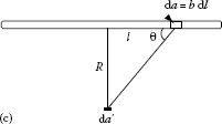
The illumination provided by a given source depends on the shape of the source and the receiver, and on their relative position. A summary of the formulae for the luminous flux and illuminance for few particular cases are presented in Table 1.2. The detailed derivation of the formulae are given in Ref. [22]. If a point source illuminates an area, and the area is tilted by the angle θ with respect to the normal of the source area, the projected area must be used. The mathematical solution of the problem of a line source, such as fluorescent lamp, and a point receiver is similar to the derivation of the Biot–Savart law for magnetisms. The luminous flux and the illuminance, at a point receiver provided by a line source, obey 1/R law of attenuation of the emitted light toward a point receiver.

1.1.3.4 Conversion between Radiometric and Photometric Units

The relation between watts and lumens is not just a simple scaling factor, because the relationship between lumens and watts depends on the wavelength. One watt of IR radiation (which is where most of the radiation from an incandescent bulb falls) is worth zero lumens. The lumen is defined only for 555 nm, that is, the definition of lumen tells us that 1 W of green 555 nm light is worth 683 lm.

The conversion between radiometric and photometric units for the other wavelengths within the visible spectrum is provided by the eye sensitivity function, V(λ), shown in Figure 1.1. The eye has its peak sensitivity in the green at 555 nm, where the eye sensitivity function has a value of unity, that is, V(555 nm) = 1. For wavelengths smaller than 390 nm and larger than 720 nm, the eye sensitivity function falls off below 10⁻³.

The conversion from watts to lumens at any other wavelength involves the product of the radiant power and the V(λ) value at the wavelength of interest. The spectral density of the radiant flux, Φ(λ) = dΦ/dλ, is the light power emitted per unit wavelength and measured in watts per nanometer, and is also called spectral power distribution. The luminous flux, Φ_λ, is related to the spectral density of the radiant flux Φ(λ) through the luminous efficiency function V(λ) measured in lumen:

$Φ_{λ} = 683 [\frac{1 m}{W}] \int_{λ} V (λ) Φ (λ) d λ$ $Φ_{λ} = 683 [\frac{1 m}{W}] \int_{λ} V (λ) Φ (λ) d λ$

(1.15)

This equation suggests that radiant flux of 1 W at a wavelength of 555 nm produces a luminous flux of 683 lm. This equation could also be used for other quantity pairs. For instance, luminous intensity (cd) and spectral radiant intensity (W/sr · nm), illuminance (lux) and spectral irradiance (W/m² · nm), or luminance (cd/m²) and spectral radiance (W/m²· sr · nm).

TABLE 1.2
Illumination by Sources with Different Geometrical Shapes

Type of Source	Luminous Flux	Illuminance
Point source and area receiver	$Φ_{λ} = I_{λ} \frac{π r^{2}}{r^{2} + R} ≅ I_{λ} \frac{π r^{2}}{R^{2}}$ $Φ_{λ} = I_{λ} \frac{π r^{2}}{r^{2} + R} ≅ I_{λ} \frac{π r^{2}}{R^{2}}$	$E_{λ} = \frac{Φ_{λ}}{π r^{2}} = L_{λ} \frac{d a}{r^{2} + R^{2}}$ $E_{λ} = \frac{Φ_{λ}}{π r^{2}} = L_{λ} \frac{d a}{r^{2} + R^{2}}$
Area source and point receiver	$Φ_{λ} = L_{λ} π \sin^{2} α d a^{'}$ $Φ_{λ} = L_{λ} π \sin^{2} α d a^{'}$	$E_{λ} = \frac{Φ_{λ}}{d a^{'}} = L_{λ} π \sin^{2} α$ $E_{λ} = \frac{Φ_{λ}}{d a^{'}} = L_{λ} π \sin^{2} α$
Line source (fluorescent lamp) and point receiver	$Φ_{λ} = L_{λ} d a^{'} (b \frac{2}{R})$ $Φ_{λ} = L_{λ} d a^{'} (b \frac{2}{R})$ , where b is the width of the line source, and (2b/R) gives the solid angle in steradians.	$E_{λ} = L_{λ} (b \frac{2}{R})$ $E_{λ} = L_{λ} (b \frac{2}{R})$
Oblique illumination: point source and point receiver	$Φ_{λ} = L_{λ} d a (\frac{d a^{'}}{R^{2}}) \cos θ$ $Φ_{λ} = L_{λ} d a (\frac{d a^{'}}{R^{2}}) \cos θ$	$E_{λ} = L_{λ} \frac{d a \cos θ}{R^{2}}$ $E_{λ} = L_{λ} \frac{d a \cos θ}{R^{2}}$
Oblique illumination: point source and area receiver	Φλ = L_λ da π sin²α cos θ	E_λ = L_λ π sin² α cos θ

Equation 1.15 represents a weighting, wavelength by wavelength, of the radiant spectral term by the visual response at that wavelength. The wavelength limits can be set to restrict the integration only to those wavelengths where the product of the spectral term Φ(λ) and V(λ) is nonzero. Practically, this means that the integration is over the entire visible spectrum, because out of the visible range, V(λ) ≅ 0 and the integral tends to zero. As the V(λ) function is defined by a table of empirical values, the integration is usually done numerically. The optical power emitted by a light source is then given by

$Φ = \int_{λ} Φ (λ) d λ$ $Φ = \int_{λ} Φ (λ) d λ$

(1.16)

Let us compare the luminous flux of two laser pointers both with radiometric power of 5 mW working at 670 and 635 nm, respectively. At 670 nm, V(λ) = 0.032 and the luminous flux is 0.11 lm (683 lm/W × 0.032 × 0.005 W = 0.11 lm). At 635 nm, V(λ) = 0.217 and the laser pointer has luminous flux is 0.74 lm (683 lm/W × 0.217 × 0.005 W = 0.74 lm). The shorter wavelength (635 nm) laser pointer will create a spot that is almost seven times as bright as the longer wavelength (670 nm) laser (assuming the same beam diameter). Using eye sensitivity function, V(λ), one can show also that 700 nm red light is only about 4% as efficient as 555 nm green light. Thus, 1 W of 700 nm red light is worth only 27 lm.

The International Commission on Weights and Measures (CGPM) has approved the use of the CIE curve for photopic (light conditions) vision V(λ) and the curve for scotopic (dark-adapted) vision V’(λ) for determination of the value of photometric quantities of luminous sources. Therefore, for studies at lower light levels, the curve for scotopic (dark-adapted) vision V′(λ) should be used. This V′(λ) curve has its own constant of 1700 lm/W, the maximum spectral luminous efficiency for scotopic vision at the peak wavelength of 507 nm. This value was chosen such that the absolute value of the scotopic curve at 555 nm coincides with the photopic curve, at the value 683 lm/W.

Converting from lumens to watts is far more difficult. As we want to find out Φ(λ) that was already weighted and placed inside an integral, we must know the spectral function Φ_λ of the radiation over the entire spectral range where the source emits not just the visible range.

The luminous efficacy of optical radiation is the conversion efficiency from optical power to luminous flux. It is measured in units of lumen per watt of optical power. The luminous efficacy is a measure of the ability of the radiation to produce a visual response and is defined as

$Luminous efficacy = \frac{Φ_{λ}}{Φ} = \frac{683 [\frac{lm}{W}] \int_{λ} V (λ) Φ (λ) d (λ)}{\int_{λ} Φ (λ) d λ} [\frac{lm}{W}]$ $Luminous efficacy = \frac{Φ_{λ}}{Φ} = \frac{683 [\frac{lm}{W}] \int_{λ} V (λ) Φ (λ) d (λ)}{\int_{λ} Φ (λ) d λ} [\frac{lm}{W}]$

(1.17)

For monochromatic light (Δλ → 0), the luminous efficacy is equal to the eye sensitivity function V(λ) multiplied by 683 lm/W. Thus, the highest possible efficacy is 683 lm/W. However, for multicolor light sources and especially for white light sources, the calculation of the luminous efficacy requires integration over all wavelengths.

The luminous efficiency of a light source is the ratio of luminous flux of the light source to the electrical input power (IV) of the device and shows how efficient the source is in converting the consumed electric power to light power perceived by the eye:

$Luminous efficiency = Φ_{λ} / (I V)$ $Luminous efficiency = Φ_{λ} / (I V)$

(1.18)

The luminous efficiency is measured in units of lumen per watt, and the maximum possible ratio is 683. Combining Equations 1.4, 1.17, and 1.18 gives that the luminous efficiency is a product of luminous efficacy and electrical-to-optical power conversion efficiency (radiant efficiency):

$Luminous efficiency = luminous efficacy \times radiant efficiency$ $Luminous efficiency = luminous efficacy \times radiant efficiency$

(1.19)

For an ideal light source with a perfect electrical-to-optical power conversion, the luminous efficiency is equal to the luminous efficacy. The luminous efficiency of common light sources varies from about 15 to 25 lm/W for incandescent sources such as tungsten filament light bulbs and quartz halogen light bulbs, from 50 to 80 lm/W for fluorescent light tubes, and from 50 to about 140 lm/W for high-intensity discharge sources such as mercury-vapor light bulbs, metal-halide light bulbs, and high-pressure sodium (HPS) vapor light bulbs [12].

As an example, let us calculate the illuminance and the luminous intensity of a standard 60 W incandescent light bulb with luminous flux of 900 lm. The luminous efficiency, that is, the number of lumen emitted per watt of electrical input power, of the light bulb is 15 lm/W. The illuminance on a desk located 1.5 m below the bulb would be E_λ = 31.8 lux and would be enough for simple visual tasks (orientation and simple visual tasks require 30–100 lux as recommended by the Illuminating Engineering Society of North America) [24,25]. The luminous intensity of the light bulb is I_λ = 71.6 lm/sr = 71.6 cd.

In addition to the luminous efficiency, another highly relevant characteristic for an LED is the luminous intensity efficiency. It is defined as the luminous flux per steradian per unit input electrical power and is measured in candela per watt. In most applications of LEDs, the direction of interest is normal to the chip surface. Thus, the luminance of an LED is given by the luminous intensity emitted along the normal to the chip surface divided by the chip area. The efficiency can be increased significantly by using advanced light-output-coupling structures [26], but it is on the expense of low luminance because only a small part of the chip is injected with current. LEDs emit in all directions, as the intensity depends on the viewing angle and the distance from the LED. Therefore, in order to find the total optical power emitted by an LED, the spectral intensity I(λ) (W/m² · nm) should be integrated over the entire surface area of a sphere A:

$Φ = \int_{A} \int_{λ} I (λ) d λ d A$ $Φ = \int_{A} \int_{λ} I (λ) d λ d A$

(1.20)

1.1.3.5 Choosing a Light Source

Several important factors determine the best type of a light source for a given application: spectral distribution, output (needed irradiance), F-number, source size and shape, and the use of a grating monochromator.

Spectral distribution: The light source should have intense output in the spectral region of interest. Arc lamps are primarily UV to visible light sources, which make them useful for UV spectroscopy and UV photochemistry applications. Mercury lamps have very strong peaks in the UV. Mercury (xenon) lamps have strong mercury lines in the UV with xenon lines in the IR, and enhancement of the low-level continuum in the visible range. Xenon flashlamps are pulsed sources of UV near-IR radiation, which are flexible, but not complicated. Figure 1.5 compares the average irradiance from a xenon DC arc lamp and a large bulb xenon flashlamp with pulse duration 9 μs. Quartz tungsten halogen lamps are a good choice for long-wave visible to near-IR applications. In addition, quartz tungsten halogen lamps deliver smooth spectra without spikes. Figure 1.6 shows the spectral irradiance of mercury, xenon, and halogen lamps.

Source power: The needed irradiance determines the choice of the source output. Besides lasers, short arc lamps are the brightest sources of DC radiation. A high power lamp is best for applications that require irradiation of a large area and when the used optics imposes no limitation. For a small target or when a monochromator with narrow slit is used, a small arc lamp may produce more irradiance because of its high radiance within a very small effective arc area. When the illuminated area is small, both the total flux and the arc dimensions are of importance. Narrow spectrograph slits require the use of collection and imaging system, which involves calculation of F-numbers.

F-number (power/nm): Lamps are used barely without lamp house containing a collimator lens. Figure 1.7 shows a lens of clear aperture D, collecting light from a source and collimating it. The source is placed at the focal length f of the lens. As most sources radiate at all angles, it is obvious that increasing D or decreasing f allows the lens to capture more light. The F-number concept puts these two parameters together in order to enable a quick comparison of optical elements. The F-number is defined as

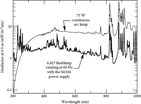
FIGURE 1.5 Comparison of average irradiance at 0.5 m from the 6251 75 W xenon DC arc lamp and the 6427 large bulb flashlamp running at 60 Hz (60 W average and pulse duration 9 μs). (Courtesy of Newport Corporation, Richmond, VA.)

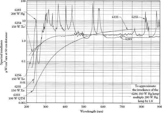
FIGURE 1.6 Spectral irradiance of Hg, Xe, and halogen lamp. (Courtesy of Newport Corporation, Richmond, VA.)

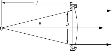
FIGURE 1.7 Lens collecting and collimating light from a source. (Courtesy of Newport Corporation, Richmond, VA.)

$F / # = \frac{1}{2 n \sin θ}$ $F / # = \frac{1}{2 n \sin θ}$

(1.21)

where

n is the refractive index of the medium in which the source is located (normally air, therefore n = 1)

θ is the angle as shown in Figure 1.7

However, the approximation is valid only for the paraxial rays (small angles θ). Therefore,

$F / # = f / D$ $F / # = f / D$

(1.22)

is widely used as F-number, even at large values of θ. The F/# is useful to convert from the irradiance data in Figure 1.6 to beam power. For example, the irradiance value for the 150 W xenon lamp at 540 nm is 2 μW/cm²/nm (see Figure 1.6). If F/1 condenser is used, the conversion factor is 0.82. The conversion factor is written in the manual of the lamp housing and might vary between different lamp suppliers. Multiplying the irradiance value with the conversion factor gives the result in milliwatt per nanometer, which for the given example is (2 μW/cm² · nm) (0.82) = 1.64 mW/nm. In a typical lamp housing, a reflector is mounted behind the lamp, which increases the lamp output by 60%. Hence, the output is (1.64 mW/nm) (1.6) = 2.6 mW/nm.

Source size and shape: The size and shape of the source, as well as the available optics, also determine the illumination of the sample. If the application requires a monochromatic illumination, a monochromator is normally placed between the lamp and the target. The object size of an arc is considerably smaller than that of a coil. Hence, with an arc lamp, more light can be guided through a monochromator in comparison with a quartz tungsten halogen lamp of the same power.

Grating monochromators: A grating monochromator permits the selection of a narrow line (quasi-monochromatic light) from a broader spectrum of incident optical radiation. Used with a white light source, a monochromator provides selectable monochromatic light over the range of several hundred nanometers for specific illumination purposes. Two processes occur within the monochromator. First, it is the geometrical optical process wherein the entrance slit is imaged on the exit slit. The second process is the dispersion process on the rotating grating. Table 1.3 shows the selecting criteria for a proper grating based on the most important operating parameters of a monochromator. The resolution is the minimum detectable difference between two spectral lines (peaks) provided by a given monochromator. While resolution can be theoretically approximated by multiplying slit width (mm) × dispersion (nm/mm), the actual resolution rarely equals this due to aberrations inherent in monochromators. The dispersion of a monochromator indicates how well the light spectrum is spread over the focal plane of the exit plane. It is expressed in the amount of wavelengths (nm) over a single millimeter of the focal plane. The aperture (or F-number) is the ratio of the focal length of the monochromator to the grating diameter, equivalent to Equation 1.22. The focal length is the distance between the slit and the focusing component of the monochromator. The bandpass (nm) is the actual resolution of a monochromator as a function of the slit width. At zero order, the grating acts as a mirror, and all incident wavelengths are reflected. For this reason, it is often helpful to use zero-order reflection when setting up an optical system. The grating linearly polarizes the light passing through the monochromator, and the degree of polarization depends on the wavelength.

TABLE 1.3
Selection Criteria of Gratings

Groove density (or groove frequency): The number of grooves contained on a grating surface (lines/mm)	Groove density affects the mechanical scanning range and the dispersion properties of a system. It is an important factor in determining the resolution capabilities of a monochromator. Higher groove densities result in greater dispersion and higher resolution capabilities. Select a grating that delivers the required dispersion when using a charge-coupled device (CCD) or array detector, or the required resolution (with appropriate slit width) when using a monochromator.
Mechanical scanning range: The wavelength region in which an instrument can operate	Refers to the mechanical rotation capability (not the operating or optimum range) of a grating drive system with a specific grating installed. Select a grating groove density that allows operation over your required wavelength region.
Blaze wavelength:The angle in which the grooves are formed with respect to the grating normal, often called blaze angle	Diffraction grating efficiency plays an important role in monochromator or spectrograph throughput. Efficiency at a particular wavelength is largely a function of the blaze wavelength if the grating is ruled, or a modulation if the grating is holographic. Select a blaze wavelength that encompasses the total wavelength region of your applications, and, if possible, favors the short wavelength side of the spectral region to be covered.
Quantum wavelength range: The wavelength region of highest efficiency for a particular grating	Normally determined by the blaze wavelength. Select a grating with maximum efficiency over the required wavelength region for your application.

Typical system configurations of light sources and monochromators for transmittance, reflectance, and emission measurements using different detectors are shown in Figure 1.8. As the emission intensity of a light source and the efficiency of a grating versus wavelength are not constant (see Figure 1.5), it is necessary to make corrections to the measured spectra. For this purpose, the response of the illuminating system, that is, monochromator and lamp, is measured with a calibrated detector. The corrected response of the measured spectrum is given by

$R_{corr} = (I_{m} / I_{D}) \times R_{D}$ $R_{corr} = (I_{m} / I_{D}) \times R_{D}$

(1.23)

where

I_m is the measured response

I_D is the reference measurement with the detector

R_D is the response function of the detector

FIGURE 1.8 Typical system configurations of light sources and monochromators. (Courtesy of Newport Corporation, Richmond, VA.)

1.1.4 PHOTOMETRIC MEASUREMENT TECHNIQUES

Photometric measurements employ photodetectors (devices that produce an electric signal when exposed to light), and the choice of the photometric method depends on the wavelength regime under study.

Photometric measurements are frequently used within the lighting industry. Simple applications include switching luminaires (light fixtures) on and off based on ambient light conditions and light meters used to measure the amount of light incident on a surface. Luminaires are tested with gonio-photometers or rotating mirror photometers. In both the cases, a photocell is kept stationary at a sufficient distance such that the luminaire can be considered as a point source. The rotating mirror photometers use a motorized system of mirrors to reflect the light from the luminaire in all directions to the photocell, while the goniophotometers use a rotating table to change the orientation of the luminaire with respect to the photocell. In either case, luminous intensity is recorded and later used in lighting design.

Three-dimensional photometric measurements use spherical photometers to measure the directional luminous flux produced by light sources. They consist of a large-diameter globe with the light source mounted at its center. A photocell measures the output of the source in all directions as it rotates about the source in three axes.

Photometry finds broad applications also in astronomy, where photometric measurements are used to quantify the observed brightness of an astronomical object. The brightness of a star is evaluated by measuring the irradiance E (the energy per unit area per unit time) received from the star or when the measurements are done with the same detecting system (telescope and detector)—the radiant flux (energy per unit time). The ancient studies of stellar brightness (by Hipparchus, and later around AD 150 by Ptolemy) divided the stars visible to the naked eye into six classes of brightness called magnitudes. The first-magnitude stars were the brightest and the sixth-magnitude stars the faintest. The later quantitative measurements showed that each jump of one magnitude corresponded to a fixed flux ratio, not a flux difference. Thus, the magnitude scale is essentially a logarithmic scale, which can be explained with the logarithmic response of the eye to brightness. It was found that a difference of 5 magnitudes (mag) corresponds to a factor of 100 in energy flux. If the radiant fluxes of two stars are Φ₁ and Φ₂, and m₁ and m₂ are the corresponding magnitudes, the mathematical expression of this statement is

$\frac{Φ_{1}}{Φ_{2}} = 100^{(m_{2} - m_{1}) / 5} = 10^{(m_{2} - m_{1}) / 2.5}$ $\frac{Φ_{1}}{Φ_{2}} = 100^{(m_{2} - m_{1}) / 5} = 10^{(m_{2} - m_{1}) / 2.5}$

(1.24)

This equation is used to calculate the brightness ratio for a given magnitude difference. It shows that each time m₂ − m₁ increases by 5, the ratio Φ/Φ₂ decreases by a factor of 100; thus, increasing the irradiance decreases the magnitude. The magnitude difference for a given brightness ratio is given by

$m_{2} - m_{1} = 2.5 \log (\frac{Φ_{1}}{Φ_{2}})$ $m_{2} - m_{1} = 2.5 \log (\frac{Φ_{1}}{Φ_{2}})$

(1.25)

The magnitude range for stars visible to the naked eye is 1–6 mag. This corresponds to a flux ratio Φ₁/Φ₂ = 10^{(6 − 1)/2.5} = 10². The largest ground-based telescopes allow to extend the magnitude range from 6 to 26 mag, which corresponds to a flux ratio Φ/Φ₂ = 10^{(26 − 6)/2.5} = 10⁸. This way, using telescopes allows creating a continuous scale that extends the original 6 mag scale to fainter or brighter objects. In this new scale, brighter objects than 1 mag can have 0 mag, or even negative magnitudes.

Photometric techniques in astronomy are based on measuring the radiant flux of the stellar object through various standard filters. The radiation from a star is gathered in a telescope, passing it through specialized optical filters (passbands), and the light energy is then captured and recorded with a photosensitive element. The set of well-defined filters with known sensitivity to a given incident radiation is called a photometric system. The sensitivity depends on the implemented optical system, detectors, and filters. The first-known standardized photometric system for classifying stars according to their colors is the Johnson–Morgan UBV (ultraviolet, blue, and visual) photometric system, which employs filters with mean wavelengths of response functions at 364, 442, and 540 nm, respectively [27]. The Johnson–Morgan technique used photographic films to detect the light response. Those films were sensitive to colors on the blue end of the spectrum, which determined the choice of the UBV filters.

Nowadays, there are more than 200 photometric systems in use, which could be grouped according to the widths of their passbands in three main groups. The broadband systems employ wide passbands, wider than 30 nm, as the most frequently used system is the Johnson–Morgan UBV system. The intermediate band and the narrow band systems have passbands widths of 10–30 and less than 10 nm, respectively. Most optical astronomers use the so-called Johnson–Cousins photometric system, which consists of ultraviolet, blue, visual, red, and infrared (UBVRI) filters and photomultiplier tubes [28,29].

For each photometric system, a set of primary standard stars is used. The light output of the photometric standard stars is measured carefully with various passbands of a photometric system. The light flux received from other celestial objects is then compared to a photometric standard star to determine the exact brightness or stellar magnitude of the object of interest. It is assumed that the direct observations have been corrected for extinction. The most often used current set of photometric standard stars for UBVRI photometry is that published by Landolt [30,31].

The apparent brightness of a star depends on the intrinsic luminosity of the star and its distance from us. Two identical stars at different distances will have different apparent brightnesses. This requires correcting the apparent brightness for the distance to the star. Starlight is also affected by interstellar extinction. Therefore, in all cases in which the distance to an astronomical object is a concern, the observer should correct for the effects of interstellar absorption. In order to compare two stars, we have to know their total luminosities (power output). If the total radiant power of a star is Φ, and if no radiation is absorbed along the way, all energy per second leaving the surface of the star will cross a sphere at a distance d in the same time. The radiant exitance of the star M = Φ/(4πr²) falls off inversely as the square of the distance. Unfortunately, distances to astronomical objects are generally hard to determine. Distances to nearby stars could be determined by a simple trigonometric method called trigonometric parallax. It is based on triangulation from two different observing points [32]. With current ground-based equipment, parallax can be measured within a few thousandths of an arc second. Parallax measurements are useful for the few thousand nearest stars. Therefore, they are the starting point for a very complex system for determining distances to astronomical objects.

Photometry was intensively used in the 1960s to determine the red shift in the spectrum of a distant astronomical object such as a galaxy or quasar. The red shift is a measure of the rate at which any galaxy is receding from us and hence, through Hubble’s law, of the distance to it [32,33]. The technique relies on the assumption that the radiation spectrum emitted by the object has strong features that can be detected by the relatively crude filters. This technique was largely replaced in the 1970s by more reliable spectroscopic determinations of red shifts [34]. Photometry is also used to measure the light variations of objects such as variable stars, minor planets, active galactic nuclei, and supernovae, or to detect transiting extrasolar planets. These measurements can be used, for example, to determine the rotation period of a minor planet or a star, the orbital period and the radii of the members of an eclipsing binary star system, or the total energy output of a supernova.

The traditional photometric methods employed photoelectric photometers, devices that measured the light intensity of a single object by focusing its light on to a photosensitive cell. The modern photometric systems use CCD cameras, which can simultaneously image multiple objects and allow to measure accurately the signal spread over many pixels due to broadening caused by the optics in the telescope and the star twinkling. The methods used to extract data from the raw CCD image depend on the observed objects. Aperture photometry is a method used to determine the radiant flux of a distant star that can be considered as a point source (an object with an angular diameter that is much smaller than the resolution of the telescope). It consists in adding up the pixel counts within a circle centered on the object and subtracting off the pixel count of the background light. When the target is a globular cluster, the individual fluxes of the overlapping sources are obtained via de-convolution techniques such as point spread function fitting. After determining the flux of an object in counts, one must calibrate the measurement. For this purpose, differential, relative, or absolute photometry can be used, depending on the type of photometric measurements, as all techniques require corrections for the atmospheric extinction when the object is observed from the ground.

Differential photometry measures the changes in the brightness of an object over time and requires corrections for temporal variations in the sensitivity of the instrument. For this purpose, a number of comparison stars, which are assumed to be constant, are simultaneously observed together with the target. In general, differential photometry provides the highest precision of photometric measurements.

Relative photometry compares the apparent brightnesses of multiple objects relative to each other. This technique requires corrections for spatial changes in the sensitivity of the instrument. If the objects being compared are too far apart to be observed simultaneously, additional corrections for their temporal variations have to be done.

Absolute photometry measures the apparent brightness of an object with a standard photometric system. Thus, in addition to the other factors mentioned above, one has to account also for the differences between the effective passband through which the object is observed and the passband used to define the standard photometric system. To provide correction for this effect, the target should be observed through multiple filters, simultaneously with a number of photometric standard stars. Due to those complications, absolute photometry is the most difficult to do with high precision.

More information about astronomical photometry could be found in specialized books and literature [35,36,37,38,39,40,41,42].

1.1.5 COLORIMETRY

Colorimetry deals with measurement of color. The fundamentals of colorimetry are presented in detail in Refs. [13,14]. Colorimetry deals with basic concepts such as tristimulus values, chromaticity coordinates, color temperature, and color rendering. Colorimetry describes colors in numbers (tristimulus values) and provides a physical color match using a variety of measurement instruments. Colorimetry utilizes the standard color science calculations and codes provided by the 1931 CIE. The description of colors by numbers is based on the fact that all colors can be represented as a combination of the three primary colors (stimuli): red, green, and blue. The tristimulus values X, Y, and Z give the amounts of each stimuli in a given color represented by the spectral power distribution Φ(λ). The numerical value of a given color is obtained by integrating the spectrum with the standard color-matching functions $\bar{x} (λ), \bar{y} (λ)$ $\bar{x} (λ), \bar{y} (λ)$ , and $\bar{z} (λ)$ $\bar{z} (λ)$ based on a 1931 CIE standard observer:

$X = \int \bar{x} (λ) Φ (λ) d λ$ $X = \int \bar{x} (λ) Φ (λ) d λ$

(1.26a)

$Y = \int \bar{y} (λ) Φ (λ) d λ$ $Y = \int \bar{y} (λ) Φ (λ) d λ$

(1.26b)

$Z = \int \bar{z} (λ) Φ (λ) d λ$ $Z = \int \bar{z} (λ) Φ (λ) d λ$

(1.26c)

The ○ $\bar{x} (λ)$ $\bar{x} (λ)$ , ■ $\bar{y} (λ)$ $\bar{y} (λ)$ , and ▲ $\bar{z} (λ)$ $\bar{z} (λ)$ color-matching functions are shown on Figure 1.9. The graph plots the tabulated values of the 1978 CIE color-matching functions, also called the Judd–Vos-modified 1978 CIE two-degree color matching functions for point sources [14,16,17,18,19,20]. The ■ color-matching function, $\bar{y} (λ)$ $\bar{y} (λ)$ , is identical to the eye sensitivity function V(λ) for photopic vision.

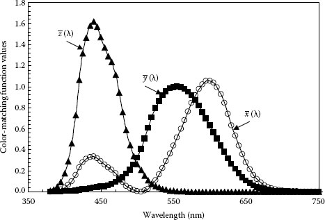
FIGURE 1.9 1978 CIE color matching functions: $\bar{x} (λ)$ $\bar{x} (λ)$ , ○; $\bar{y} (λ)$ $\bar{y} (λ)$ , ■; and $\bar{z} (λ)$ $\bar{z} (λ)$ , ▲. (Adapted from Schubert, E.F., Light-Emitting Diodes, Cambridge University Press, Cambridge, U.K., 2003.)

The chromaticity coordinates (x, y) are functions of the tristimulus values X, Y, and Z and describe quantitatively the color of a radiating light source with a spectrum Φ(λ):

$x = \frac{X}{X + Y + Z}$ $x = \frac{X}{X + Y + Z}$

(1.27a)

$y = \frac{Y}{X + Y + Z}$ $y = \frac{Y}{X + Y + Z}$

(1.27b)

$z = \frac{Z}{X + Y + Z} \equiv 1 - x - y$ $z = \frac{Z}{X + Y + Z} \equiv 1 - x - y$

(1.27c)

As the coordinate z can be expressed by the other two, every color could be represented by only two independent chromaticity coordinates (x, y) in a two-dimensional graph called chromaticity diagram. The 1931 CIE chromaticity diagram [5,43,44] provides simple means of color mixing. A set of n primary sources with chromaticity coordinates (x_i, y_i) and radiant fluxes Φ_i will produce a color with chromaticity coordinates (x_c, y_c) which are given by

$x_{c} = \frac{\sum_{i = 1}^{n} x_{i} Φ_{i}}{\sum_{i = 1}^{n} Φ_{i}} and y_{c} = \frac{\sum_{i = 1}^{n} y_{i} Φ_{i}}{\sum_{i = 1}^{n} Φ_{i}}$ $x_{c} = \frac{\sum_{i = 1}^{n} x_{i} Φ_{i}}{\sum_{i = 1}^{n} Φ_{i}} and y_{c} = \frac{\sum_{i = 1}^{n} y_{i} Φ_{i}}{\sum_{i = 1}^{n} Φ_{i}}$

(1.28)

The radiant fluxes Φ_i of the primary sources used in these equations should be normalized so that the sum X_i + Y_i + Z_i equals unity for all i.

Colorimetry is a basic method for describing light sources in lighting industry. Depending on the nature of the emission processes, different light sources emit different spectra. As a way of evaluating the ability of a light source to reproduce the colors of various objects being lit by the source, the CIE introduced the color rendering index (CRI; 1974 CIE and updated in 1995), which gives a quantitative description of the lighting quality of a light source [45,46]. After reflecting from an illuminating object, the original radiation spectrum is altered by the reflection properties of the object, that is, the object’s reflectivity spectrum. This results in a shift of the chromaticity coordinates, the so-called colorimetric shift. As reflectivity spectra will produce different colorimetric shifts for different spectral composition of the source, colors may appear completely different from, for instance, colors produced by sunlight. To estimate the quality of lighting, eight test samples are illuminated successively by the source to be tested and by a reference source. The reflected spectra from the samples are determined and the chromatic coordinates are calculated for both the tested and the reference sources. Then, the colorimetric shifts are evaluated and graded with respect to chromatic adaptation of the human eye using the 1960 CIE uniform chromaticity scale diagram and the special CRI R_i for each sample is calculated. The general CRI R_a is obtained by averaging of the values of the eight special CRI R_i:

$R_{a} = \frac{1}{8} \sum_{i = 1}^{8} R_{i}$ $R_{a} = \frac{1}{8} \sum_{i = 1}^{8} R_{i}$

(1.29)

This method of grading of colorimetric shifts obtained in test samples is called CIE test-color method, and is applicable for light sources that have chromaticity close to the reference illuminant. The CRI is a measure of how well balanced the different color components of white light are. A standard reference illuminant has a general CRI R_a = 100. The two primary standard illuminants are the CIE Standard Illuminant A (representative of tungsten-filament lighting with color temperature of 2856 K) and the CIE Standard Illuminant D65 (representative of average daylight with color temperature of 6500 K). Color rendering is a very important property of cold illuminants such as LEDs and discharge lamps, whose emission spectrum contains certain wavelengths. More information about the test-color samples, standard colorimetric illuminants and observers, and CRIs can be found in related references [3,5,24,45] and CIE reports [47,48,49,50], as well as in the literature on LEDs [9,10,11].

The measurements of color light sources (lamps, LEDs, and displays) involve spectroradiometers and tristimulus colorimeters. In order to characterize the color, lamps are usually measured for spectral irradiance, whereas displays are measured for spectral radiance. When a spectroradiometer is designed to measure spectral irradiance (W/m²·nm), it is equipped with a diffuser or a small integrating sphere as input optics, while a spectroradiometer, which is designed to measure spectral radiance (W/sr · m²· nm), employs imaging optics. A spectroradiometer could be one of a mechanical scanning type, which are more accurate but slow, or of diode-array type, which are fast, but less accurate devices. Spectroradiometers are calibrated against spectral irradiance and radiance standards [49], which suggest that their measurement uncertainty is determined first by that of the reference source. Other factors influencing the measurement uncertainty are wavelength error, detector non-linearity, bandwidth, stray light of monochromator, measurement noise, etc. [44]. Tristimulus colorimeters are used to calibrate display devices and printers by generating color profiles used in the workflow. Accurate color profiles are important to ensure that screen displays match the final printed products. Tristimulus colorimeters are low-cost and high-speed devices, but their measurement uncertainty tend to be higher than spectroradiometers.

A colorimeter can refer to one of the several related devices. In chemistry, a colorimeter generally refers to a device that measures the absorbance of a sample at particular wavelengths of light. Typically, it is used to determine the concentration of a known solute in a given solution by the application of the Beer–Lambert law, which states that the concentration of a solute is proportional to the absorbance. Colorimetry finds wide area of applications in chemistry and in industries such as color printing, textile manufacturing, paint manufacturing, and in the food industry.

Colorimetry is also used in astronomy to determine the color index of an astronomical object. The color index is a simple numerical expression of the color of an object, which in the case of a star gives its temperature. To measure the color index, the object is observed successively through two different sets of standard filters such as U and B, or B and V, centered at wavelengths λ₁ and λ₂, respectively. The difference in magnitudes found with these filters is called U–B or B–V color index. For example, the B–V color index corresponding to the wavelengths λ_B and λ_V is defined by

$m_{B} - m_{V} = 2.5 \log [\frac{I (λ_{V})}{I (λ_{B})}] + constant$ $m_{B} - m_{V} = 2.5 \log [\frac{I (λ_{V})}{I (λ_{B})}] + constant$

(1.30)

where I(λ_V) and I(λ_B) are the intensities averaged over the filter ranges. If we suppose that an astronomical object is radiating like a blackbody, we need to know only the ratio of brightnesses at any two wavelengths to determine its temperature. The constant in Equation 1.30 is adjusted so that m_B − m_V is zero for a particular temperature star, designated as A0. The ratio of blue to visible intensity increases with the temperature of the object. This means that the m_B − m_V color index decreases. The smaller the color index, the more blue (or hotter) the object is. Conversely, the larger the color index, the more red (or cooler) the object is. This is a consequence of the logarithmic magnitude scale, in which brighter objects have smaller magnitudes than dimmer objects. For example, the yellowish Sun has a B − V index of 0.656 ± 0.005 [51], while the B − V color index of the bluish Rigel is −0.03 (its B magnitude is 0.09 and its V magnitude is 0.12, B − V = −0.03) [52]. The choice of filters depends on the object’s color temperature: B − V are appropriate for mid-range objects, U − V for hotter objects, and R − I for cool objects. Bessel specified a set of filter transmissions for a flat response detector, thus quantifying the calculation of the color indices [53].

1.2 LIGHT EMISSION

Light can be emitted by an atomic or molecular system when the system, after being excited to a higher energy level, decays back to a lower energy state through radiative transitions. The excitation of the system can be achieved by different means: thermal agitation, absorption of photons, bombarding with high-speed subatomic particles, and sound and chemical reactions. Additional excitation mechanisms such as radioactive decay and particle–antiparticle annihilation result in emission of very-high-energy photons (γ-rays). The following description of emission processes and light sources is not intended to be comprehensive. More details about the different excitation mechanisms, the resultant emission pocesses, and light sources could be found in specialized books [54,55,56,57,58,59,60,61,62,63].

1.2.1 BLACKBODY RADIATION

The most common light sources are based on thermal emission, also called incandescence (from Latin “to grow hot”). Incandescence is the radiation process, which results from the de-excitation of atoms or molecules after they have been thermally excited. A body at a given temperature emits a broad continuum of wavelengths, for example, sunlight, incandescent light bulbs, and glowing solid particles in flames.

A blackbody is a theoretical model that closely approximates many real objects in thermodynamic equilibrium. A blackbody is an ideal absorber (absorbs all the radiation impinging on it, irrespective of wavelength or angle of incidence), as well as a perfect emitter. A blackbody at constant temperature radiates energy at the same rate as it absorbs energy; thus, the blackbody is in thermodynamic equilibrium. The balance of energy does not mean that the spectrum of emitted radiation should match the spectrum of the absorbed radiation. The wavelength distribution of the emitted radiation is determined by the temperature of the blackbody and was first described accurately by Max Planck in 1900. The empirical formula for the spectral exitance M_λ of a blackbody at temperature T(K), derived by Planck is

$M_{λ} = \frac{2 π h c^{2}}{λ^{5}} [\frac{1}{\exp (h c / λ k_{B} T) - 1}]$ $M_{λ} = \frac{2 π h c^{2}}{λ^{5}} [\frac{1}{\exp (h c / λ k_{B} T) - 1}]$

(1.31)

The spectral exitance M_λ is the power per unit area per unit wavelength interval emitted by a source. The constant h is called Planck’s constant and has the numerical value h = 6.62606876 × 10⁻³⁴ J · s, k_B = 1.3806503 × 10⁻²³ J/K = 8.62 × 10⁻⁵ eV/K is Boltzmann’s constant, and c = 2.99792458 × 10⁸ m/s is the speed of light in vacuum. In order to provide a theoretical background for this relation, Planck postulated that a blackbody can only radiate and absorb energy in integer multiples of hv. That is, the energy could only be emitted in small bundles, or quanta, each quanta having energy hv and frequency ν. The explanation of the quantization in the process of radiation and absorption was proposed by Albert Einstein in 1905.

Figure 1.10 shows blackbody spectra for six temperatures. At any wavelength, a hotter blackbody gives off more energy than a cooler blackbody of the same size. Also, as the temperature increases, the peak of the spectrum shifts to shorter wavelengths. The relation between the wavelength at which the peak λ_max occurs and the temperature T is given by Wien’s displacement law:

$λ_{\max} T = \frac{h c}{5 k_{B}} = 2.898 \times 10^{3} μ m \cdot K$ $λ_{\max} T = \frac{h c}{5 k_{B}} = 2.898 \times 10^{3} μ m \cdot K$

(1.32)

This relation can be derived from Equation 1.31 by differentiating M_λ with respect to λ and setting it equal to zero. The curve illustrating Wien’s law is shown on Figure 1.10 with a dashed line.

Integrating the spectral exitance from Equation 1.31 over all wavelengths gives the total radiant exitance, M, which is also the area under the blackbody radiation curve at temperature T:

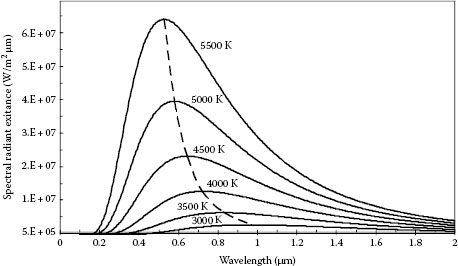
$M = \int_{0}^{\infty} M_{λ} d λ = σ T^{4}$ $M = \int_{0}^{\infty} M_{λ} d λ = σ T^{4}$

(1.33)

FIGURE 1.10 Blackbody radiation at six temperatures (K). Solid curves show the spectral distribution of the radiation. The dashed curve connecting the peaks of the six solid curves illustrates Wien’s displacement law.

where σ = 5.6703 × 10⁻⁸ W/m²· K⁴ is the Stefan–Boltzmann constant. According to Equation 1.33, known as Stefan–Boltzmann law, the radiant exitance (the total energy per unit time per unit surface area) given off by a blackbody is proportional to the fourth power of the temperature.

Sun and stars, as well as blackened surfaces, behave approximately as a blackbody. Blackbody sources (blackened cavities with a pinhole) are commercially available at operating temperatures from −196°C (liquid nitrogen) to 3000°C. Sun emits thermal radiation covering all wavelengths of the electromagnetic spectrum. The surface temperature of Sun is around 6000 K and the emitted radiation peaks in the visible region. Other stellar objects, like the great clouds of gas in the Milky Way, also emit thermal radiation but as they are much cooler, their radiation is in the IR and radio regions of the electromagnetic spectrum. In astronomy, the radiant flux, Φ, or the total power given off by a star is often referred as luminosity. The luminosity of a spherical star with a radius R and total surface area 4πR² is

$Φ = \int M d a = (4 π R^{2}) σ T^{4}$ $Φ = \int M d a = (4 π R^{2}) σ T^{4}$

(1.34)

The luminosity of Sun, calculated for surface temperature about 6000 K and radius of 7 × 10⁵ km, is about 4 × 10²⁶ W. This quantity is called a solar luminosity and serves as a convenient unit for expressing the luminosity of other stars.

The color of light sources is measured and expressed with the chromaticity coordinates. But when the hue of white light source has to be described, it is more practical to use the correlated color temperature (CCT) in Kelvin instead of the chromaticity coordinates. The term “color temperature” originates from the correlation between temperature and emission spectrum of Planckian radiator. The radiation from a blackbody is perceived as a white light for a broad range of temperatures from 2,500 to 10,000 K but with different hues: for example, a blackbody at 3,000 K radiates white light with reddish hue, while at 6,000 K the light adopts a bluish hue. The CCT is used to describe the color of white light sources that do not behave as blackbody radiators. The CCT of a white source is the temperature of a Planckian radiator whose perceived color is closest to the color of the white light source at the same brightness and under specified viewing conditions [44,50]. For example, 2800 K is associated with the warm color of incandescent lamps, while the color temperature of quartz halogen incandescent lamps is in the range from 2800 to 3200 K [45].

1.2.2 LUMINESCENCE

Luminescence is a nonthermal radiation process that occurs at low temperatures and is thus a form of cold body radiation. Nonthermal radiators are known as luminescent radiators. Luminescence differs from incandescence in this that it results in narrow emission spectra at shorter wavelengths, which correspond to transitions from deeper energy levels. Luminescence can be manifested in different forms, which are determined by the mechanism or the source of excitation: photoluminescence (PL), electroluminescence, cathodoluminescence, chemiluminescence, sonoluminescence, bioluminescence, triboluminescence, etc.

1.2.2.1 Photoluminescence

PL results from optical excitation via absorption of photons. Many substances undergo excitation and start glowing under UV light illumination. PL occurs when a system is excited to a higher energy level by absorbing a photon and then spontaneously decays to a lower energy level, emitting a photon. When the luminescence is produced in a material by bombarding with high-speed subatomic particles such as β-particles and results in x- or γ-ray radiation, it is called radioluminescence. An example of a common radioluminescent material is the tritium-excited luminous paints used on watch dials and gun sights, which replaced the previously used mixture of radium and copper-doped zinc sulfide paints.

1.2.2.2 Fluorescence

Fluorescence is a luminescence phenomenon in which atom de-excitation occurs almost spontaneously (<10⁻⁷ s) and in which emission ceases when the exciting source is removed. In fluorescent materials, the radiative transitions are one-step process that takes place between energy states with the same spin (with equal multiplicity):

$E * \to E + h v$ $E * \to E + h v$

(1.35)

Here the transition from an excited state E* to the ground or lower energy state E consists of emission of a photon of frequency ν and energy hν (h is the Planck’s constant). The couple of states E* and E could be singlet–singlet or triplet–triplet. The amplification of fluorescence by stimulated emission is the principle of laser action. The quantum yield of a fluorescent substance is defined by the number of reemitted photons to the total number of absorbed photons:

$ϕ = \frac{number of reemitted photons}{number of absorbed photons}$ $ϕ = \frac{number of reemitted photons}{number of absorbed photons}$

(1.36)

1.2.2.3 Phosphorescence

Phosphorescence is a luminescence phenomenon from spin-forbidden transitions (e.g., triplet–singlet), and the emission of light persists after the exciting source is removed. Phosphorescence is a two-step process that could be described as

$S_{0} + h ν \to S_{1} \to T_{1} \to S_{0} + h ν^{'}$ $S_{0} + h ν \to S_{1} \to T_{1} \to S_{0} + h ν^{'}$

(1.37)

where

S and T denote a singlet and a triplet state, respectively

hν′ is the emitted photon

hν is the absorbed photon

Subscripts “0” and “1” indicate the ground state and the first excited state, which is given here only for simplicity because transitions can also occur to higher energy levels, respectively.

The excited electrons become trapped in the triplet state (a metastable state) for prolonged period of time, which causes substantial delay between excitation and emission. Although most phosphorescent compounds de-excite rather quickly (on the order of milliseconds), there are certain crystals as well as some large organic molecules, which remain in a metastable state sometimes as long as several hours. These substances effectively store light energy, and if the phosphorescent quantum yield is high, they release significant amounts of light over long time, creating an afterglow effect. The metastable states could be populated also via thermal excitation; therefore, phosphorescence is temperature-dependent process. Common pigments used in phosphorescent materials include zinc sulfide and strontium oxide aluminate. Since strontium oxide aluminate has a luminance approximately 10 times greater than zinc sulfide, it is used widely in safety-related signage (exit signs, pathway marking, and other).

1.2.2.4 Multiphoton Photoluminescence

Multiphoton PL occurs when a system is excited by absorption of two or more photons of the same or different energies, followed by emission of one photon of which energy can be greater than the energy of one of the exciting photons. Two-photon PL is the most often used process. In this process, two identical photons of energy hν₁ are absorbed by the system, which spontaneously de-excites emitting a photon with energy larger than the energy of the absorbed photons (hν₂ = 2hν₁). If the decay includes a non-radiative relaxation to an intermediate energy level, the energy of the fluorescence photon is hν₂ < 2hν₁. Two-photon absorption is a nonlinear optical process that depends on the impinging intensity and occurs preferentially where the intensity of light in the sample is the greatest. When two-photon PL is used to study biological samples, one should have in mind that the longer wavelength of the excitation photons allows for greater depth of penetration into the sample. Therefore, in order to avoid damage of biological samples, the average intensity of the excitation beam should be sufficiently low. At the same time, the peak intensity of the excitation beam should be high enough to ensure two-photon absorption. Such conditions can be provided by a mode-locked laser working in femtosecond pulse regime; the ultrashort optical pulses provide very short time of interaction of light with the biological tissue, as well as high-peak power but low-average power of the excitation beam.

A popular imaging technique known as two-photon laser scanning fluorescence microscopy employs two-photon fluorescence to obtain higher resolution than ordinary microscopy [57,58]. The method uses a fluorescent probe (fluorophore) linked to specific location in the sample. The excitation beam is focused on the fluorescent probe providing conditions for two-photon absorption. The probe absorbs a pair of photons incident on it and emits a single photon of larger energy, which is detected. The two-photon absorption rate at the position of the probe, along with the emission rate, is proportional to the square of the impinging intensity [58,59,60,61,62]. This results in a stronger signal from the area in focus and much weaker fluorescence background from the out-of-focus area. In addition, the image is sharper and the resolution is higher than the ordinary microscopy based on single-photon absorption.

Another application of multiphoton absorption is the three-dimensional micro-lithography. The method employs specially designed transparent polymers with strong polymerization nonlinearity. A micro-object can be created in the volume of the polymer matrix by focusing high-power optical pulses at the location of interest. The intensity of the focused beam is high enough to initiate multiphoton polymerization only in the vicinity of the focal point. A computer-generated threedimensional microstructure can be transferred into the polymer matrix by moving the focal point of the lens to follow the desired shape.

Figure 1.11 illustrates upconversion fluorescence process used to convert IR photons to visible photons. The system, usually phosphors doped with rare-earth ions, is excited by two-photon absorption of an auxiliary photon of energy hν₁ and an IR photon of low energy hν₂. A rare-earth ion such as Er³⁺ can trap the electron excited by the first photon till the arrival of the second photon, which brings the electron to the upper energy level via sequential absorption. If there is no non-radiative relaxation involved, the energy of the resultant luminescence photon is equal to the sum of energies of both absorbed photons, hν₃ = hν₁ + hν₂. One practical application of upconversion fluorescence is for viewing an IR laser beam using an IR sensor card. The card can be reflective or transmissive and consists of upconverting phosphor powder laminated between a pair of stiff transparent plastic sheets. Viewing the spatial distribution of an IR beam is important when aligning IR lasers or optical systems using such lasers.

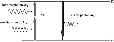
FIGURE 1.11 Upconversion fluorescence process.

PL occurs in all forms of matter, and it is a very useful tool for investigating the optical properties such as temperature dependence of absorption coefficient and energy position of the bandgap of semiconductor materials. In fact, PL measurements have been used to study absorption and emission of CdS and GaAs [63,64]. The model used to explain the experimental data underlies the detailed balance principle and is expressed by the modified Roosbroeck–Shockley equation considering self-absorption [64]:

$I (T, h ν) \propto {(h ν)}^{2} {1 - \exp [- α (T, h ν) d]} \exp (- h ν / k T_{c})$ $I (T, h ν) \propto {(h ν)}^{2} {1 - \exp [- α (T, h ν) d]} \exp (- h ν / k T_{c})$

(1.38)

where

I is the emitted light intensity

hν is the photon energy

d is the active sample thickness, which corresponds to the diffusion length of the minority carriers

k is the Boltzmann constant

α is the absorption coefficient

T is the lattice temperature

T_c is the actual carrier temperature (the carrier temperature might exceed considerably the lattice temperature T_c ≫ T)

Figure 1.12 shows PL spectra (solid lines) of bulk p-type (≈10¹⁸ cm⁻³ GaAs). The PL spectra were measured in the temperature range 5–300 K [64], using an argon laser as optical excitation and the data were recorded with a Fourier transform infrared Bomen spectrometer. The broken lines represent the fits to the PL spectra using Equation 1.38, while the absorption coefficient has been modeled with density of states and Urbach’s rule. Figure 1.13 shows the variation of the bandgap according to the PL spectra shown in Figure 1.12. The solid line is calculated with a vibronic model, pointing to the fact that the band-gap energy in semiconductors depends much stronger on the electron–lattice interaction rather than on volume changes. The squares correspond to the PL maxima in Figure 1.12 and the solid dots to the values calculated from Equation 1.38 in conjunction with the modeled absorption coefficient [64].

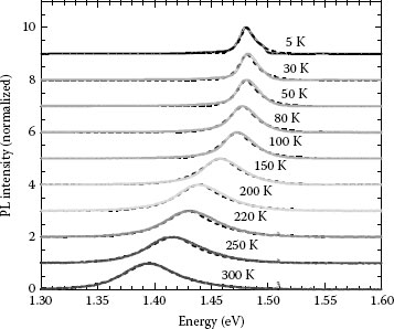
FIGURE 1.12 PL spectra (solid line) and fits (broken line) according to Equation 1.38. For clarity, the spectra are normalized and shifted. (From Ullrich, B. et al., Semicond. Sci. Technol., 22, 1174, 2007. With permission.)

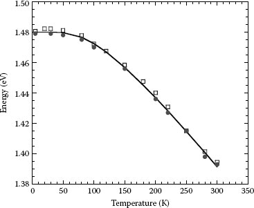
FIGURE 1.13 Bandgap energy of p-type GaAs versus temperature. The solid line represents the fit with the vibronic model used in Ref. [56], whereas the squares correspond to the PL maxima in Figure 1.12, and the dots are the bandgap values found from Equation 1.38. (From Ullrich, B. et al., Semicond. Sci. Technol., 22, 1174, 2007. With permission.)

Because of the strong luminescence that direct band-gap semiconductors such as CdS, ZnS, GaAs, or GaN exhibit, they are most easily examined by luminescence techniques. But indirect semiconductors such as silicon can be examined as well. Although they emit light at much weaker level, the luminescence of dislocated silicon is different from intrinsic silicon and can be used to localize defects in integrated circuits.

1.2.2.5 Electroluminescence

Electroluminescence is the light emission when electric field is applied to a material. Electro-luminescence in semiconductors results from radiative recombination of electrons from the conduction band with holes from the valence band. Prior to recombination, electrons and holes are separated either by doping of the material to form a p−n junction (as in electroluminescence devices such as LEDs) or through excitation by impact of high-energy electrons accelerated by a strong electric field. When the emission is triggered by an electric current injected into a forward-biased p−n junction, as in the case of LEDs, the process is called injection electroluminescence [65,66]. Examples of electroluminescent materials include III–V semiconductors, such as InP, GaAs, and GaN, powder zinc sulfide doped with copper or silver, thin-film (TF) zinc sulfide doped with manganese, organic semiconductors, natural blue diamond (diamond with boron as a dopant), etc. In crystals such as diamonds, the source of luminescence can be lattice defects.

Electroluminescence devices have lower power consumption than neon signs and find broad applications in advertising boards and safety signs. Electroluminescent panels based on powder phosphor provide a gentle, even illumination and are frequently used as backlights to liquid crystal displays (LCDs). The low-electric-power consumption makes them convenient for battery-operated devices such as pagers, wristwatches, and computer-controlled thermostats. Recently, blue, red, and green emitting TF electroluminescent materials have been developed that offer the potential for long life and full color electroluminescent displays. Electroluminescent lamps can be made in any color. However, the most commonly used are of greenish color because they provide the greatest luminous efficiency (the greatest apparent light output for the least electrical power input).

1.2.2.6 Cathodoluminescence

Cathodoluminescence is the emission of light after excitation by impact of high-energy electrons. The impingement of energetic electrons generated by a cathode-ray tube, like in the case of a TV screen or an image intensifier (used in night vision devices), onto a luminescent material (phosphor or a semiconductor) results in the promotion of electrons from the valence band into the conduction band, leaving behind a hole. The recombination of an electron and a hole can be radiative process with emission of a photon or non-radiative process with creation of a phonon. The energy (color) of the emitted photon and the probability that a photon will be emitted, not a phonon, depend on the material and its purity.

Cathodoluminescence finds applications in geology, mineralogy, materials science, and semiconductor engineering. It can be implemented in an optical or electron microscope with the proper accessories to examine the optical properties of nonmetallic materials such as semiconductors, minerals, ceramic, glass, etc. The depth of penetration into a sample can be modified by changing the electron energy. As different components in a material produce emission at different wavelengths, cathodoluminescence is used to study the material structure in order to get information on its composition, growth, and quality. For this purpose, a scanning electron microscope with specialized optical detectors or an optical cathodoluminescence microscope is most often used [67,68,69,70]. The choice of the microscope technique depends on the application. An electron microscope with a cathodoluminescence detector has much higher magnification and versatility but is more complicated and more expensive compared to an optical cathodoluminescence microscope, which is easy to use and shows actual visible color features immediately through the eyepiece. Other advantages of the scanning electron microscope are high resolution (10–20 nm), the ability to detect the entire spectrum at each point (hyperspectral imaging) if a CCD camera is used, and the ability to perform nanosecond to picosecond time-resolved spectroscopy if the electron beam can be chopped into nanosecond or picosecond pulses. These advantages are important when examining low-dimensional semiconductor structures, such as quantum wells or quantum dots.

1.2.2.7 Sonoluminescence

Sonoluminescence is the emission of short bursts of light from a gaseous cavity (bubbles) induced in a liquid by high-intensity sound [71,72]. The light emission occurs when the bubbles quickly collapse and reach minimum size. Sonoluminescence can be observed from clouds of bubbles and, under certain circumstances, from a single bubble [73,72,73,74,75,76]. The bubble may already exist in the liquid or may be created through cavitation, the process of formation, growth, and collapse of bubbles under the influence of high-intensity sound or ultrasound. A single bubble can be trapped at a pressure antinode of the acoustic standing wave formed in the liquid. It will periodically expand and collapse, emitting a flash of light each time it collapses. Single-bubble flashes can have very stable periods and positions. The resonant frequencies depend on the shape and size of the container. The light pulses from the bubbles are extremely short (between 35 and a few hundred picoseconds) [76]. Adding a small amount of noble gas (helium, argon, or xenon) to the gas in the bubble increases the intensity of the emitted light. The collapsed bubbles are about 1 μm in diameter depending on the ambient fluid (e.g., water) and on the gas content of the bubble (e.g., atmospheric air). When the bubble collapses, the pressure increases significantly and the temperature in the interior of the bubble can reach around 10,000 K. This causes ionization of the noble gas present in the bubble [74]. Such high temperatures provide conditions for thermonuclear fusion. This possibility makes sonoluminescence especially interesting subject for investigation [77].

1.2.2.8 Chemiluminescence

Chemiluminescence is the emission of light as a result of excitation via a chemical reaction. Under certain circumstances, the energy released during a chemical reaction might be sufficient to excite the reaction product, which fluoresces as it decays to a lower energy level. For example, one typical chemiluminescence reaction is the luminol reaction:

$Luminol + H_{2} O_{2} \to 3 -APA* \to 3-APA + light$ $Luminol + H_{2} O_{2} \to 3 -APA* \to 3-APA + light$

(1.39)

Luminol in an alkaline solution with hydrogen peroxide (H₂O₂) in the presence of a suitable catalyst (iron or copper, or an auxiliary oxidant) produces chemiluminescence. The energy released in the reaction is sufficient to populate the excited state of the reaction product 3-aminophthalate (3-APA*), which de-excites to 3-APA emitting a photon. In the ideal case, the number of the emitted photons should correspond to the number of molecules of the reactant. However, the actual quantum efficiency of nonenzymatic reactions, as in this case, seldom exceeds 1%. The luminal reaction is an example of liquid-phase reaction [78,79].

One of the oldest known chemoluminescent reactions is that of elemental white phosphorus oxidizing in moist air, producing a green glow (gas-phase reaction). Another type of chemical reactions produces chemiluminescence from a fluorescent dye or fluorophor, which is incorporated in the chemical mixture of reactants. The reaction can be described as Reactant 1 + Reactant 2 + dye → Products + dye*, where dye* is the excited state of the dye. The most common example of this type of reaction is the glow of lightsticks. They emit steady glow for up to 12 h and are used for emergency indications, as well as for illumination in underwater and military environment. The chemical reaction by which the lightsticks work is

$Cyalume + H_{2} O_{2} + dye \to Phenol \to {2CO}_{2} + dye*$ $Cyalume + H_{2} O_{2} + dye \to Phenol \to {2CO}_{2} + dye*$

(1.40)

The chemicals are kept in separated compartments (for storage purposes). Once the reactants are permitted to mix, the energy of the reaction activates the fluorescent dye, which decays to a lower energy level emitting light. This is the most efficient nonenzymatic chemiluminescence reaction known. A typical organic system useful for chemiluminescence exhibits a quantum efficiency of about 23% compared with about 3% for the best-known aqueous systems [78,79,80]. The color, intensity, and duration of the emitted light are determined by the fluorescent dye. Some of the most common dyes are 9,10-diphenylanthracene emits blue light, tetracene emits yellow–green light, rhodamine 6 G gives bright orange light with moderate duration of emission, while rhodamine B emits red light.

Chemiluminescence is an important tool for gas analysis, for instance, for determining the content of ozone, nitric oxides, sulfur compounds, or small amounts of impurities or poisons in air. In environmental air-quality testing, the concentration of nitric oxide can be detected down to 1 ppb by using chemiluminescence techniques. Other applications of chemiluminescence include analysis of inorganic species in liquid phase, analysis of organic species, DNA sequencing using pyrosequencing, etc. Enhanced chemiluminescence is a common technique in biology. It allows detection of minute quantities of a biomolecule and femtomole quantities of proteins, which are well below the detection limit for most assay systems.

1.2.2.9 Bioluminescence

Bioluminescence is the chemiluminescence produced by living organisms such as bacteria, fireflies, glowworms, and jellyfish. Some studies suggest that 90% of deep-sea marine organisms produce bioluminescence in one form or another. Although, certain fish emit red and IR lights, most marine light-emission is in blue region of the spectrum where seawater is transparent. Non-marine or land bioluminescence is less distributed, as the two best-known examples are fireflies and New Zealand glowworms. Bioluminescence results from enzyme-catalyzed chemiluminescence reactions that can reach the highest known quantum efficiency for a chemiluminescence reaction (88% for the firefly), whereas synthetic reactions can provide only a 23% efficiency at best [80,81]. Bioluminescent organisms are intensively studied for better understanding of behavioral mechanisms (means of communication), as well as because of potential applications of engineered bioluminescence such as new methods for detecting bacterial contamination of meats and other foods, bio-identifiers, etc.

1.2.2.10 Triboluminescence

Triboluminescence is the light generated via the breaking of asymmetrical bonds in a crystal when that material is scratched, crushed, or rubbed (from the Greek tribein “to rub”). For example, many minerals, such as quartz, glow when scratched; sucrose emits a blue light when crushed; and a diamond may begin to glow while being sawn during the cutting process or a facet is being ground. Diamonds may fluoresce blue or red. The mechanism of triboluminescence is not fully understood yet, but the research in this area suggests that charge is separated upon fracture of asymmetrical materials and when the charges recombine, the electric discharge ionizes the surrounding air, causing a flash of light [82].

1.2.2.11 Scintillation

Scintillation is the emission of short light pulses from certain chemical compounds after being excited by charged particles or by photons of high energy. Scintillation is an inherent molecular property of conjugated and aromatic organic molecules but can occur also in inorganic materials. Ionizing particles passing through organic scintillators excite the molecules to deep energy levels, which upon relaxation emit UV light. The emitted spectra are characteristic for the electronic structure of the molecules. By adding a sensitizer (wavelength-shifting molecules), the UV photons are converted into visible light. Examples of organic scintillators include crystals such as anthracene (C₁₄H₁₀) and naphthalene (C₁₀H₈); organic liquids (usually have brand names such as PPO, POPOP, PBD, etc.); and plastics—a solid solvent, doped with aromatic compounds (TP, PPO, or PBD) or with wavelength shifters, such as polysterene and polyvinyltuolene. Examples of inorganic scintillators are crystals such as NaI(Tl), CsI(Tl), and BaF₂, and gaseous and liquid scintillators on the base of Xe, Kr, Ar, He, or N. Inorganic materials find application in high-precision calorimetry. In chemistry, calorimetry is used to determine the heat released or absorbed in a chemical reaction and specific heat capacities of liquids. In particle physics, a calorimeter is an experimental apparatus that measures energy of charged particles.

Scintillation counters measure ionizing radiation and are used in high-energy physics experiments for timing, for fast event selection, or for measuring the energy of charged particles by total absorption in sampling calorimeters. Each charged particle passing through the scintillator produces a flash, as the intensity of the light flash depends on the energy of the charged particles. The scintillation counter apparatus consists basically of a scintillator and a photomultiplier with the counter circuits. A scintillation counter can be used also as a spectrometer to determine the energy of x-ray or γ-photons causing scintillation by measuring the intensity of the flash (the number of lower energy photons produced by the high-energy photon). Cesium iodide (CsI) in crystalline form is used as the scintillator for the detection of protons and α-particles, while sodium iodide (NaI) containing a small amount of thallium is used as scintillator for the detection of γ-particles.

Light yield (or light gain) is an important parameter of scintillation counters. It is a measure of the scintillation efficiency, and shows how much of the energy of a charged particle or a high-energy photon in the scintillation counter is converted into visible light. For historical reasons, anthracene is used as a standard for light gain. The light yield of anthracene crystals is of the order of 5% for blue light or about two photons per 100 eV for high-energy particles. For comparison, the inorganic crystal NaI has a light yield of about 230% of anthracene, while typical plastic scintillators exhibit light yield of 50%–60% [83].

1.3 CONVENTIONAL LIGHT SOURCES

Conventional light sources employ either incandescence or electrical discharge in gases. Both phenomena come along with large energy losses, due to the inherent involvement of high temperature and large Stokes shifts (the emitted photons are with lower energy than the absorbed photons), which result in relatively low luminous efficiencies.

1.3.1 INCANDESCENT LAMPS AND TUNGSTEN HALOGEN LAMPS

Incandescent lamps utilize electric current to heat a material (tungsten filament) and produce light by incandescence. The spectrum of incandescent lamps depends on the operating temperature of the tungsten filament. The peak of the tungsten spectrum is shifted to smaller wavelengths providing higher luminous efficacy than a blackbody radiator. This blue shift, though, does not affect the color rendering, which remains almost the same as a Planckian radiator. The main portion of the radiation is in the IR part of the spectrum. The radiation losses in addition to heat losses (in the lead wires from the wire surface into the surrounding gas) reduce the luminous efficiency of this type of light sources. The overall efficiency of a 120 V/100 W lamp is only about 7%, which means that only about 7% of the consumed energy is converted into useful visible radiation and the remainder as IR radiation. Light output (lm) depends both on the filament temperature and the electrical input power (wattage). A 120 V incandescent lamp working at CCT of 2790 K and consuming 60 W electric power provides a luminous flux of 865 lm and luminous efficiency about 14.4 lm/W [5]. An incandescent lamp has a CRI R_a = 100 and exhibits color rendering properties identical to the standard reference illuminant. The efficiency of the incandescent lamps depends on the voltage: the higher the voltage, the less efficient the lamp is. The incandescent lamps have very short lifetime, typically less than 1000 h. During operation, tungsten gradually evaporates from the filament and deposits as a dark film on the inner bulb surface. This can decrease the light output by as much as 18% during the life of the lamp. The efficiency and the lifetime can be increased by reducing the tungsten evaporation rate by the addition of halogen vapor (iodine or bromine) to the gas filling of the lamp. The halogen bounds with the evaporated tungsten and forms tungsten halide, which diffuses back to the filament, reducing the evaporation effect and providing higher operational temperatures (as high as 3450 K). A typical tungsten halogen lamp has at least twice longer lifetime of an incandescent lamp at the same efficiency. Figure 1.14 compares the spectral exitance of an Oriel quartz tungsten halogen lamp with a blackbody radiator. A 120 V/50 W tungsten halogen lamp at operation temperature of 2750 K, provides a luminous flux of 590 lm and has luminous efficiency of about 11.8 lm/W and CRI R_a = 100 [5]. Incandescent and tungsten halogen lamps are of interest mainly for residential lighting and motor vehicle headlights. The tungsten filament lamp is also a popular light source for optical instrumentation designed to use continuous radiation in the visible and into the IR regions.

More recently, modified FEL 1000 W quartz halogen lamps were tested for suitability as photometric transfer standards, and they were shown to be stable within 0.2%–0.6% over 60 h of operation. Of special interest for calibration is the quartz tungsten halogen lamp standard of Gamma Scientific, Inc., Model 5000-16C 1000 W FEL lamp standard. It provides absolute calibration of spectral radiance from 250 nm to 2.5 μm. This lamp standard has been selected by the National Institute of Standards and Technology (NIST) to replace the 1000 W, DXW standard. It is calibrated to the 1973 NIST spectral irradiance scale, while the DXW standard is calibrated to the 1965 NIST scale [84]. The lamp calibration is directly traceable to NIST by incorporating two NIST spectral irradiance scales. This results in estimated accuracies of 2.4% at 250 nm, 1.8% at 450 nm, and 1.5% over the range from 555 to 1600 nm. The 1965 NIST scale of spectral irradiance is used over the spectral range from 1700 to 2500 nm, as NIST uncertainty over this wavelength region is approximately 3%.

Quartz tungsten halogen lamps emit down to 240 nm. At the operating high wattages, the emitted UV radiation is hazardous. Therefore, the user of these sources has to wear UV protective glasses and gloves.

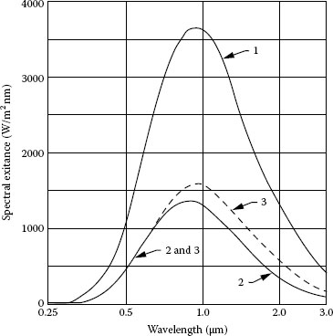
FIGURE 1.14 Spectral exitance of (1) blackbody radiator, (2) a tungsten surface, and (3) a gray body with emissivity of 0.425, all at 3100 K. (Courtesy of Newport Corporation, Richmond, VA.)

1.3.2 GAS DISCHARGE LAMPS

Gas discharge lamps utilize an electrical discharge through an ionized gas to generate light. Typically, such lamps are filled with a noble gas (argon, neon, krypton, and xenon) or a mixture of these gases, as most lamps contain also vapors of mercury, sodium, and metal halides. Sodium and mercury are efficient low-pressure discharge emitters. When a large enough electric field is applied to the gas in the lamp, the gas partially ionizes producing conductive plasma, which contains free electrons, ions, and neutral particles. The character of the gas discharge depends on the frequency of the electric current. The gas discharge could be stabilized by limiting the electric current via a ballast. The inert gas determines the electrical characteristics of the gas discharge, mainly by controlling the mean path traveled by electrons between collisions. The source of the electrons may be a heated cathode (thermionic emission), a strong field applied to the cathode (field emission), or the impact of positive ions on the cathode (secondary emission). The electrons, accelerated by the applied electric field, collide inelastically and excite the gas and metal vapor atoms, which may relax by emitting visible or UV light. To increase the luminous efficiency, the inner surface of the glass tube of some lamps is covered with a fluorescent coating of varying blends of metallic and rare-earth phosphor salts, which converts the UV radiation to visible light.

Gas discharge lamps working at high pressure and high current produce broad spectral continuum with pronounced spectral line characteristics of the vapor. At lower pressure and current, the spectral output consists of sharper spectral lines with minimal background continuum. As each gas has a characteristic emission spectrum of certain wavelengths, different gas discharge lamps may reproduce differently the colors of various surfaces being lit by the source. An important characteristic of cold illuminants is the CRI, which is used to evaluate the color reproduction ability of a light source. Gas discharge lamps have indexes below 100, which means that the colors appear different from the colors seen under sunlight or other standard illuminant. In general, gas discharge lamps offer longer life and higher light efficiency than incandescent lamps, but exhibit poorer color rendering and are more complicated to manufacture.

1.3.2.1 Low-Pressure Discharge Lamps

1.3.2.1.1 Fluorescent Lamps

Fluorescent lamps are low-pressure gas discharge lamps, commonly used in lighting industry. A fluorescent lamp consists of a glass or quartz tube with two electrodes at each end, filled with an inert gas (most often argon or neon, and sometimes xenon or krypton) containing low-pressure mercury vapor as an active ingredient. A typical mixture contains about 1% or even as little as 0.1% metal vapor, and 99%–99.9% inert gas. The pressure of the metal vapor is around 0.5–0.8 Pa. Mercury emits in the UV at wavelengths of 253.7 nm (about 65% of the emitted light) and 185 nm (about 10%–20%). White light is produced by stimulated fluorescence in a phosphor coating on the inner surface of the tube. The UV photons emitted by the mercury vapors are absorbed by the phosphors, which fluoresce giving off lower frequency photons that combine to produce white light.

The spectral output and color-rendering properties of the fluorescent lamps depend on the emission spectra of the used phosphors. For example, daylight fluorescent lamps use a mixture of zinc beryllium silicate and magnesium tungstate. The phosphors should exhibit high quantum efficiency (more than 85%) in addition to other requirements for structural and chemical stability. There are three main groups of fluorescent lamps based on the employed phosphors: halophosphate phosphors, triphosphors, and multiband phosphors. The oldest fluorescent lamps employ calcium halophosphate phosphor, Ca₅(PO₄)₃(Cl, F):(Sb³⁺, Mn²⁺). The spectrum contains mainly blue and yellow light (480 and 580 nm), corresponding to the emission lines of the antimony ions and the manganese ions, as the green and red content is very limited [5,25]. To the eye, this mixture appears white, but the spectrum is incomplete, which explains the poor color rendering (R_a = 50–76). The triphosphors, developed in the 1970s, comprise three components that provide the three primary colors, the combination of which gives white light. A variety of matrices doped with rare-earth europium and terbium ions are used: for example, Y₂O₃:Eu³⁺ emits red; CeMgAl₁₁O₁₉:Tb³⁺, GdMgB₅O₁₀:Ce³⁺, Tb³⁺, and LaPO₄:Ce³⁺, Tb³⁺ emit green; and BaMg₂Al₁₆O₂₇:Eu²⁺ and Sr_5−x−yBa_xCa_y(PO₄)₃Cl:Eu²⁺ emit blue color. A triphosphor fluorescent lamp yields higher quantum efficiency, longer lifetime, and better color rendering (R_a = 80–85) than halophosphates, but still distorts colors because of the three narrow emission lines [25]. The multiband phosphors comprise up to five phosphors—triphosphors (for blue and green colors), halophosphates, and Mn²⁺-activated pentaborate, which emits a broad red band peaking at about 620 nm. The multiband phosphors have the highest CRIs (R_a > 90) [5]. The poorer color rendering of real-life fluorescent lamps to incandescent lamps (R_a = 100) is compensated by the higher luminous efficiency. Low-power fluorescent lamps (4–5 W) have luminous efficiency in the range from 35 to 50 lm/W (for comparison, an incandescent lamp of 10 W has luminous efficiency of 8 lm/W), while high-power linear lamps (70–125 W) reach luminous efficiency from 70 to 100 lm/W.

The overall efficiency of conversion of electric energy consumed in a fluorescent lamp to visible light at optimal conditions is about 28%. Due to losses as heat in the discharge, the walls, and the electrodes, only about 63% of the consumed electric energy is converted to UV radiation, and due to non-radiative transitions and large Stokes shift, only about 40% of the UV radiation reaching the phosphor is converted to visible light. Although low, the efficiency of a fluorescent lamp is about four times higher than a 100 W incandescent bulb of an equivalent brightness. However, the light output of a fluorescent lamp depends strongly on the ambient temperature. Fluorescent lamps operate best around room temperature as the optimal working range is between 10°C and 35°C, where the normalized luminous flux reaches about 90% [5,25]. At temperatures below freezing, it falls off to about 25% (at −20°C) and standard fluorescent lamps may not start. Therefore, special fluorescent lamps might be needed for outdoor use in cold weather. The lifetime of fluorescent lamps depends on the construction and ranges from 5,000 to 24,000 h, which is about 10–20 times as long as an equivalent incandescent lamp. A 32 W fluorescent triphosphor lamp at an operation temperature of 4100 K provides a luminous flux of 2850 lm, luminous efficiency of 84 lm/W, and CRI R_a = 78 [5]. Fluorescent lamps are the most common lamps in office lighting, and the general lighting resource in industrial and commercial environment.

1.3.2.1.2 Compact Fluorescent Lamps

Compact fluorescent lamps (CFLs) are well known as effective energy-saving light source. They are of the same size as an incandescent bulb and are made to fit the regular incandescent sockets. They utilize electronic ballasts, which do not produce light flicker. The higher initial cost is compensated by lower energy consumption over its life. Therefore, nowadays, CFLs become very popular in residential lighting. However, there is one inconvenience: the common CFL cannot be connected to a standard dimmer switch used for incandescent lamps. A 15 W CFL at an operation temperature of 2700 K provides a luminous flux of 900 lm, luminous efficiency of 51 lm/W, and CRI R_a = 82 [5].

1.3.2.1.3 Low-Pressure Sodium and Mercury Lamps

The low-pressure sodium (LPS) arc lamps are filled with neon at a pressure of 400–2000 Pa (3–15 torr) as the sodium vapor pressure is kept at 0.7–1 Pa (5–8 × 10⁻³ torr) at operating temperatures. These lamps need a long warm-up time. Upon switching on, the discharge starts in the neon and the sodium vapor pressure reaches optimal value after 10–15 min. To facilitate starting, small amounts of argon, xenon, or helium are added to the neon. The LPS lamps emit almost monochromatic light. The spectrum consists of a doublet (D-line) of two very close yellow lines at wavelengths 589.0 and 589.6 nm. Because of the high monochromaticity of the D-line, LPS lamps are commonly used for calibration and research. A 90 W LPS lamp at an operation temperature of 1,800 K provides a luminous flux of 12,750 lm, luminous efficiency of 123 lm/W, and CRI R_a = −44 [5].

The low-pressure mercury discharge lamps when used with filters can also provide strong monochromatic radiation at wavelengths of 404.7 and 435.8 nm (violet), 546.1 nm (green), and 577.0 and 579.1 nm (yellow). The low-pressure mercury and LPS lamps are used in applications that require high spectral purity.

The luminous efficacy of the D-line of the LPS lamps is 530 lm/W. The high monochromaticity of the D-line suggests extremely high theoretical efficiency of the LPS lamp. Although, 60%–80% of the input power is lost in heat and IR radiation, the LPS lamps have the highest luminous efficiencies (100–200 lm/W) among the present practical lamps. The light output of LPS lamps is in the range of 1,800–33,000 lm for wattage of 18–180 W. However, the LPS lamps exhibit very poor color rendering (R_a = −44). Therefore, from the point of view of lighting applications, LPS lamps are appropriate only for street illumination and security lighting. Lifetime is typically 14,000–18,000 h.

1.3.2.2 High-Pressure Discharge Lamps

High-pressure discharge lamps, also called high-intensity discharge (HID) lamps produce light by means of an electric arc between tungsten electrodes housed inside a transparent fused quartz or fused alumina tube. The tube is filled with inert gas and metal salts. The operating pressure is around 1 atm and higher. At such high pressure, the temperature of the plasma reaches 4000–6000 K, the interaction between the heavy particles (atoms and ions) in the plasma is enhanced, resulting in high rate of elastic collisions and collision broadening of the emission spectral lines. The HID lamps exhibit continuous spectral output with spectral lines characteristic for the metal vapors, and therefore, considerably improved color rendering in comparison to the low-pressure discharge lamps. This group includes high-pressure mercury-vapor (HMPV) lamps (the oldest type of high-pressure lamps), metal-halide lamps, HPS discharge lamps, xenon and mercury–xenon arc lamps, etc.

1.3.2.2.1 High-Pressure Mercury-Vapor Lamps

High-pressure mercury-vapor lamps work at operating pressures from 0.2 to 1 MPa (2–10 atm). The spectrum emitted from the mercury vapor at such high pressure consists of a broad continuous background overlaid with spectral lines of longer wavelengths (404.7, 435.8, 546.1, 577.0, and 579.1 nm). Because of deficiency of red color, a clear mercury lamp has a very poor CRI (R_a = 16). A phosphorus coating on the inner wall of the lamp, typically europium-activated yttrium vanadate, improves the color rendering (up to 50), as well as the luminous efficiency. In HPMV lamps, more than half of the consumed power is lost in heat and UV photon down-conversion. A 250 W high-pressure mercury lamp at an operation temperature of 3,900 K provides a luminous flux of 11,200 lm, luminous efficiency of 34 lm/W, and CRI R_a = 50 [5]. Lifetime may reach 24,000 h, and failure is usually due to loss of emission from the electrodes. Because of their lower luminous efficiency, HPMV lamps have been replaced in most applications by metal-halide lamps and HPS lamps.

1.3.2.2.2 Metal-Halide Lamps

Metal-halide lamps are high-pressure mercury lamps with added metal halides to improve the luminous efficiency and color rendering. As the excitation energy of the additive metals (about 4 eV) is lower than that of mercury (7.8 eV), the metal halides can produce a substantial amount of light and thus alter the emitted spectrum. The emission spectrum can be modified by varying the halide composition: for example, line spectra can be obtained by introducing sodium, scandium, thallium, indium, cesium, and rare-earth iodides, whereas tin or tin–sodium halides (iodides with addition of bromides and chlorides) produce more continuous spectra. The luminous efficiency is 70–110 lm/W, depending on the wattage (from 20 to 18,000 W) and additive metals used. CRIs are typically above 60 and may reach 95 for some rare-earth compounds. A 400 W fluorescent triphosphor lamp at an operation temperature of 4100 K provides a luminous flux of 2850 lm, luminous efficiency of 84 lm/W, and CRI R_a = 78 [5]. The lifetime is 2,000–30,000 h. HID lamps are typically used when high light levels over large areas are required. Since metal-halide lamps produce well-balanced white light with high brightness, they are widely used in indoor lighting of high buildings, parking lots, shops, roadways, and sport terrains.

1.3.2.2.3 High-Pressure Sodium Discharge Lamps

HPS discharge lamps contain sodium at pressure about 7000 Pa. The higher sodium pressure improves the color rendering but decreases the luminous efficiency and lifetime. The luminous efficiency of HPS lamps ranges from 60 to 130 lm/W for a typical output of 50–1000 W, respectively. Color rendering (R_a = 20–25), although higher than the LPS lamps, is still too poor. Typical lifetime is about 24,000 h. HPS lamps produce a broad spectrum, which contains a dip at the wavelengths of the D-line (self-reversed spectral lines). Because of the broader spectrum peaking in the range of the highest sensitivity of the human eye, these lamps are used mainly for street lighting, as well as for artificial photo-assimilation for growing plants.

1.3.2.2.4 Xenon and Mercury–Xenon Arc Lamps

Xenon arc lamps provide smooth continuum from near UV through the visible and into the near IR with pronounced xenon lines between 750 and 1000 nm. As xenon lamps produce bright white light that closely mimics natural daylight, they are appropriate for applications involving solar simulation, in projection systems, as well as absorbance and fluorescence research that require high-intensity broadband sources. The mercury–xenon arc lamps have essentially the mercury spectrum with xenon’s contribution to the continuum in the visible and some strong xenon lines in the near IR. Xenon and mercury–xenon arc lamps operate at very high pressure and temperature, and therefore, have to be handled with care to avoid contamination of the bulb and thermal stress. They emit strong UV radiation and require proper safety measures: protective goggles and gloves, and the lamp must be operated in a fully enclosed housing.

1.3.2.2.5 Flash Tubes

Flash tubes are pulsed high-output broadband UV–near-IR sources for which radiation results from a rapid discharge of stored electrical energy in a tube containing typically a xenon gas. For example, Oriel xenon flashlamps emit short microsecond pulses (Figure 1.15) with relatively high UV output, can operate from low frequencies up to 100 Hz, and provide maximum pulse energy of 5 J at frequencies up to 12 Hz. The short pulses find applications in lifetime and kinetic studies. Xenon flash lamps and arc lamps are often used for optical pumping of solid-state lasers (i.e., Nd:YAG).

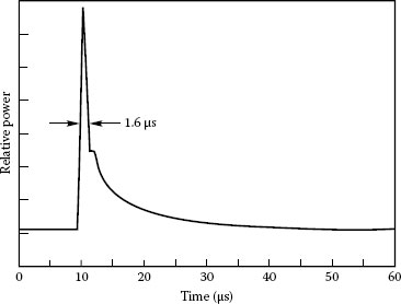
FIGURE 1.15 Pulse shape of 6426 Oriel xenon flashlamp. (Courtesy of Newport Corporation, Richmond, VA.)

More detailed information about the construction, principle of operation, transport mechanism, advantages, and disadvantages of the lighting sources considered above can be found in specialized books [5,24,25,85,86].

..................Content has been hidden....................

You can't read the all page of ebook, please click here login for view all page.

Table of Contents for Chapter 1 Light Sources

Create new playlist

Sign In

Sign Up

Table of Contents for
Chapter 1 Light Sources