15	Length and Size
	René Schödel

CONTENTS

15.1    Introduction

15.2    Basic Principle of Length Measurements by Interferometry

15.3    Basic Types of Length Measuring Interferometers

15.3.1    Twyman–Green Interferometers

15.3.2    Fizeau Interferometers

15.3.3    Fringe-Counting Interferometers

15.4    Requirements for Accurate Length Measurements by Interferometry

15.4.1    Light Sources

15.4.2    Generation and Alignment of Plane Waves

15.4.3    Determination of the Refractive Index of Air

15.4.4    Importance of Temperature Measurements

15.5    Interferometry on Prismatic Bodies

15.5.1    Imaging of the Body onto a Pixel Array

15.5.2    Interferogram Analysis

15.5.3    Length Evaluation

15.5.4    Examples of Precise Length Measurement Applications

15.6    Additional Corrections and Their Uncertainties

15.6.1    Optics Error Correction

15.6.2    Surface Roughness and Phase Change on Reflection

15.6.3    Wringing Contact between a Body and a Platen

15.6.4    Platen Flexing

15.7    Conclusions

References

15.1    INTRODUCTION

The provision of length standards and the ability to measure length to a required accuracy are of fundamental importance to any technologically developed society. Throughout history, there have been many standards for length beginning with simple definitions based on the human body, for example, cubit and feet. The continuing refinement of standards led to more specific definitions and more accurate methods of realizing them. As a milestone, in 1887, Michelson proposed the use of optical interferometers for the measurement of length. However, it needed many years until the meter was defined in terms of the vacuum wavelength of light from a krypton lamp. In 1960, this definition replaced the International Prototypes deposited in 1889 at the Bureau International des Poids et Mesures (BIPM), where they remain today. Since 1983, the meter, one of the seven base units of the SI, is defined as the length of the path traveled by light in vacuum during a time interval of 1/299,792,458 of a second [1]. This definition is based on the availability of primary frequency standards (atomic clocks) defining a second accurately. It opens two alternative ways for the realization of length measurements: (1) propagation delay: the length l is the path traveled in vacuum by a plane electromagnetic wave in time t, which is obtained using the relation l = c₀t, and the value of the speed of light in vacuum c₀ = 299,792,458 m s^–1; (2) interferometry: by means of the vacuum wavelength λ₀ of a plane electromagnetic wave of frequency f, which is obtained from the relation λ₀ = c₀/f.

The frequency of atomic clocks serving as primary standards can be transferred to frequencies of laser radiation used in length measurements by optical interferometry. This transfer is realized by frequency chains or more modern techniques utilizing femtosecond laser frequency combs. There are two ways for providing laser sources whose frequency is traceable to the SI. The common way is the use of recommended radiations generated by lasers whose frequencies are stabilized to selected hyperfine absorption lines. Currently, 12 reference frequencies covering the visible and infrared regions of the electromagnetic spectrum are recommended by the Comité International des Poids et Mesures (CIPM) [1]. As an alternative to the usage of recommended radiations, the laser light source may be directly synchronized with the primary frequency standard by femtosecond laser frequency combs.

The practical realization of length measurements depends upon the application. The propagation delay method is basically useful for long distances, for example, in space, while for the calibration of secondary length standards, for example, gauge blocks, interferometry by means of known wavelengths is preferable. The length of these primary calibrated material artifacts basically transfers the SI unit of the length to the industry and society to be used subsequently in mechanical calibrations based on comparison length measurements. Almost any relevant usage of length standards is applied under air, that is, not under vacuum conditions. Accordingly, the primary calibration of the material artifacts has to be performed under air; otherwise, the length is affected by the air pressure due to the material’s compressibility. This means that the actual relations l = ct and λ = c/f have to be considered in the primary calibration measurements. Here, the speed of light is reduced by the refractive index n of air according to c = c₀/n. Accordingly, the accurate evaluation of the air refractive index is one of the key points for the transition from the SI definition of the meter to the actually provided length standards. Other key points regard the use of adjustment methods to make sure that the SI definition is realized properly, for example, that plane waves are used. Besides these points, the laser frequency itself is no longer the limiting factor regarding length measurement uncertainty, provided that stabilized lasers are used as mentioned earlier [2]. This conclusion even holds for measurements under vacuum conditions. Therefore, the often found designation of stabilized lasers serving as secondary frequency standards as “primary length standards” is misleading.

15.2    BASIC PRINCIPLE OF LENGTH MEASUREMENTS BY INTERFEROMETRY

The basic principle of length measurement by interferometry is the comparison of a mechanical length (or a distance in space) against a known wavelength of light. Commonly, the optics is arranged such that the light beam double-passes the required length. Therefore, the measurement units are half-wavelengths, and the length being measured is expressed as

$l=\left(i+q\right)\frac{\lambda }{2},$

(15.1)

where

λ is the wavelength

i is the integer order

q is the fractional order of interference

The idea of expressing the length as multiples of the half-wavelength bases on the observation of interference intensities of two or multiple light waves is written as

$I=I_0\left[1+\text{γ}\cos \left(\frac{2\pi }{\lambda /2}\left(z_1-z_2\right)\right)\right]$

(15.2)

in the case of two-beam interference. Here, γ is the interference contrast, and z₁ – z₂ represents the geometrical distance difference between the pathways of the two beams. Thus, a change of one of the path lengths changes the interference intensity periodically in units of λ/2. The phase difference 2π/(λ/2)(z₁ – z₂) in Equation 15.2 may be expressed in terms of the vacuum wavelength, that is, by 2π/(λ₀/2) n (z₁ – z₂). Here, n is the (air) refractive index within the path, and n (z₁ – z₂) represents the difference between the two optical pathways instead of difference between the geometrical distances.

While the fractional order of interference, q, is mostly extracted from a measured interferogram, the integer order of interference, i, is usually derived from other measurements or using multiple wavelengths as described in Section 15.5.3.

The wavelength of visible light is typically 400–700 nm, and hence, the basic unit of measurement is 200–350 nm in size. By careful measurement and analysis of the interference orders (fringes), measurement uncertainties of less than 1/1000 of a fringe can be achieved with sophisticated interferometers. Extension of the wavelength range toward smaller wavelengths has the potential of obtaining picometer uncertainties under vacuum conditions. However, limitations in the practical realization, for example, due to interferometer alignment, remain the same, and new limitations may appear such as the nonavailability of appropriate monochromatic light sources or problems with optical components.

15.3    BASIC TYPES OF LENGTH MEASURING INTERFEROMETERS

15.3.1    TWYMAN–GREEN INTERFEROMETERS

The Twyman–Green interferometer is a Michelson interferometer using a collimated beam. The beam is split into two beams: one reaching a reference mirror and the other an object under test. Each beam is reflected and split again at the beam splitter, resulting in interference. The interference pattern (interferogram) is usually observed at the interferometer’s output. When the object under test is represented by a flat mirror, and the tilt angles with respect to each incident beam are the same, the entire field of view appears homogeneously illuminated and appears bright in cases of a path difference of mλ/2, and dark for differences of (m + (1/2))λ/2, where m is an integer. This situation changes when one of the mirrors is tilted. In this case, straight fringes appear along the field of view, the number and orientation of which are strongly dependent on the tilt. When the object under test is not ideally flat, the fringes are generally bent and no longer equally spaced. Such fringe pattern may be used for qualitative testing of surfaces as well as for quantitative analysis of surface topographies.

For length measurements, a prismatic body can be set in the measurement pathway as indicated in Figure 15.1. The back face of the body is attached to a platen acting as plane mirror as the front face does. The lateral offset of the fringes as shown in Figure 15.1 directly indicates the fractional order of interference, while the integer order is unsearchable because of the interferogram discontinuity induced by the length of the body.

Unwanted secondary reflection from the beam splitter’s second side can be suppressed by an antireflection coating. However, even small residual reflections lead to disturbing interferences. An effective way to eliminate the secondary reflection is to use a wedged beam splitter. This makes the direction of the secondary reflection different from the main direction, and the resulting secondary spot in the focal plane of the focusing lens can be blocked by an aperture of appropriate size. The wedge angle ε of the beam splitter causes a small deflection between the interfering beams, that is, ε(n_BS – 1), where n_BS is the refractive index of the beam splitter. When using a single wavelength, this deflection is compensated by appropriate adjustment of the reflecting surfaces. However, when multiple wavelengths are used, the dispersion of the beam splitter causes a variation of the number of observed fringes. This dispersion effect can be compensated by inserting a wedged compensation plate into the reference pathway, the wedge angle, its orientation, and the substrate material of which have to be identical with those of the beam splitter. It should be mentioned that the arrangement shown in Figure 15.1 is the only possibility. Here, the reflecting surface of the beam splitter is directed to the reference mirror. Even though in the opposite case the dispersion effect can be compensated as well, both plates together constitute a parallel plate, that is, the separation of the unwanted secondary reflection at the beam splitter is negated causing unwanted secondary interferences.

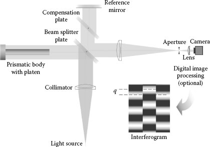
FIGURE 15.1  Diagram of a Twyman–Green interferometer. A prismatic body is placed in the measurement pathway. Unwanted reflections, for example, from the back sides of the beam splitter, can be eliminated by using wedged plates in combination with an aperture in the focal point of the first output lens. The inset shows a typical interferogram covering the body and the platen that illustrates how the fractional order of interference, q, can be extracted visually.

When the reference pathway is shifted, any fringes within the interferogram will move according to Equation 15.2. This is applied in phase-stepping interferometry [3], which is useful in large field Twyman–Green interferometers equipped with camera systems [4]. In such an approach, a number of interferograms are recorded at different but equally spaced positions along the reference pathway. From such a set of interferograms, the interference phase topography can be calculated by appropriate algorithms. In this way, the fractional order of interference, and therefore the length, can be obtained more accurately as with fringe evaluation techniques using single interferograms [5]. An example of applying phase-stepping interferometry in length measurements is given in Section 15.5.2.

A more compact interferometer design, called “Kösters–Zeiss interference comparator,” is obtained when a Kösters prism is used instead of a “normal” beam splitter [6] (see Figure 15.2). Such design is particularly useful for length measurements of relatively long prismatic bodies, for example, gauge blocks of 1 m in length. The vacuum cell shown in Figure 15.2 enables direct comparison of the path length in vacuum with the length of the optical path of air surrounding the cell. Since the air pathway is situated next to the length bar, the refractive index of air resulting from these path length differences almost coincides with that of the light pathway along the bar.

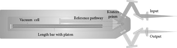
FIGURE 15.2  Diagram of the Kösters–Zeiss interference comparator.

15.3.2    FIZEAU INTERFEROMETERS

Fizeau interferometers are common large field interferometers requiring a minimum of optical components as shown in Figure 15.3. A single beam entering the interferometer is semi-reflected at the first surface, while the other is mostly totally reflecting. Multiple beams are generated by multiple reflections and can be separated from the incident beam by a beam splitter plate for analysis of the multibeam interference. Alternatively, when using two semi-reflecting surfaces, the transmitted interference may be observed, although its contrast is clearly smaller than that of the reflected interference. As in the Twyman–Green interferometer, a number of fringes are observed when there is a tilt between the reflecting faces. However, the intensity distribution of the fringes, described by the well-known airy formula, is sensitive to the reflectivity R of the semi-reflecting surface as indicated in Figure 15.3, that is, the shape is similar to a cosine (see Equation 15.2) for small values of R, while at large values, sharp peaks can be observed. As mentioned earlier, unwanted reflections leading to disturbing interferences can be eliminated by using wedged flats as optical components (including the beam splitter) in combination with an aperture.

Length measurements with a Fizeau interferometer can be performed similarly as with the Twyman–Green interferometer by inserting a prismatic body attached to a platen (see Figure 15.1) and determining the fractional order of interference from a displacement of fringes. When applying phase-stepping interferometry by recording and processing a number of interferograms at equally spaced faces positions, it is recommended to use a special algorithm [7] for Fizeau interference instead of using an algorithm designed for the two-beam interference. Errors are generated otherwise.

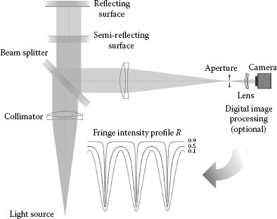
FIGURE 15.3  Diagram of a Fizeau interferometer.

The Fizeau interferometer can be extended to a double-ended version applying two reversely directed light sources [8]. In such a design, a prismatic body with reflecting surfaces (without platen) is set between two semi-reflecting faces. The length of the body can then be determined from the difference of the distance between the semi-reflecting faces and the sum of distances with respect to the body’s faces at each side, where each distance is obtained from the relevant interferogram. One application of such length measurement is the determination of the volume of cuboids in the so-called cube interferometer.

Another double-ended Fizeau interferometer is the so-called spheres interferometer [9]. Here, spherical waves are used together with spherical semi-reflecting reference faces to determine a diameter topography from which the volume of spheres can be obtained highly accurately.

15.3.3    FRINGE-COUNTING INTERFEROMETERS

These dynamic types of interferometers provide relative measurements of distances, which is given attention to in Chapter 16. Here, just a few remarks relating to absolute length measurements are made: when such systems are used to define a length, accurate setting at two defined points is required. In the measurement of absolute lengths, the optical path difference of the fringe-counting interferometer must be increased by a distance equal to the length of the object to be measured. This can be done by traversing a mirror on a linear stage between two points coincident with the two ends of the object. Fringe-counting interferometers can be found as heterodyne systems where the beat between two separated laser frequencies is observed [10]. This technique is highly appropriate for the primary calibration of line scales as interpolation errors are reduced. Another variation of the fringe-counting technique is the combination with white light interferometry. In this case, interference can be observed only when the optical path length difference between the interfering beams is around zero. This criterion can be used to define certain positions along a displacement pathway.

15.4    REQUIREMENTS FOR ACCURATE LENGTH MEASUREMENTS BY INTERFEROMETRY

15.4.1    LIGHT SOURCES

The availability of a monochromatic light source is one of the key points when interferometry is applied for length measurements. Before laser radiation entered the laboratories, it was a big challenge to generate monochromatic light from other light sources, for example, from special spectral lamps. Although specific spectral lamps still belong to the recommended light sources, they almost disappeared, these light sources meanwhile almost disappeared, while the list of stabilized laser radiations recommended by the CIPM is growing from time to time. One example of a recommended radiation is the radiation of a frequency-doubled Nd:YAG laser, stabilized with an iodine cell external to the laser, having a cold-finger temperature of −15°C. Here, the absorbing molecule is ¹²⁷I₂, and the transition is the a₁₀ component, R(56) 32-0 at a frequency of 563,260,223,513 kHz corresponding to a vacuum wavelength of 532.245036104 nm with a relative standard uncertainty of 8.9 × 10⁻¹².

There is a close link between the spectral linewidth of a light source and temporal coherence. Accordingly, it is not surprising that stabilized laser light sources as mentioned earlier have superior long coherence times. Temporal coherence is an important criterion for the observation of interference in length measurements as the interfering beams travel different lengths.

The size of the light source is also important in length measurements by interferometry. This regards different aspects as (1) the divergence of the beam affects the length measurements as discussed in Section 15.4.2 and (2) the emittance of the finite light source is desired to be large. When an aperture or a pinhole is used to reduce the size of the light source, as necessary with spectral lamps, the signal-to-noise ratio of the interference intensity signals is limited by the pinhole size, (3) the spatial coherence of the light beam. This in principle means the ability of the beam to interfere with a shifted copy of the beam. Spatial coherence is necessary when interference is formed between different parts of beams as in a shearing interferometer. A nearly perfect point source, for example, monochromatic light coming from a single-mode fiber, will generate maximum spatial coherence. On the other hand, spatial coherence is not necessary when using a non-sheared Twyman–Green arrangement together with rectangular incidence of the beams to the plane reflecting faces. In fact, in the case of the Twyman–Green interferometer, it is even advantageous that spatial coherence can be reduced. This can be done in order to lower the risk of parasitic interferences generated by any additional reflections within the interferometer’s beam path. An advisable light source generating reduced spatial coherence is a multimode fiber end. The mode field intensity distribution in such case reveals a characteristic grain as shown in the photograph in Figure 15.4a. Figure 15.4b shows the intensity distribution observed when the fiber is vibrated at 500 Hz by a speaker’s membrane.

In order to illustrate the effect of parasitic interferences, Figure 15.5 shows phase topographies resulting from measurements in a Twyman–Green interferometer equipped with a 16-bit CCD-camera system applying phase-stepping interferometry. The phase topographies each resulting from eight interferograms, recorded at 0.5 s exposure, show the total field of view of approximately 60 mm when an almost ideal optical flat is inserted and aligned so that zero fringes are observed (fluffed out mode). Figure 15.5a shows the interference phase topography when a single-mode fiber is used as light source. In this case, obscure vertical variations appear, the amplitude of which is about ±0.03 interference orders corresponding to about ±8 nm (λ ≅ 532 nm). Figure 15.5b shows the same field of view when the single-mode fiber is replaced by a vibrated multimode fiber as light source. The parasitic interference pattern disappears in the latter case, and the remaining optics error of the interferometer becomes visible.

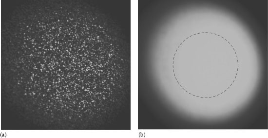
FIGURE 15.4  Photographs of light that traveled through a multimode fiber (exposure time: 50 ms); (a) original grain pattern; (b) mixed grain pattern generated by fiber vibration. The dashed circle indicates the selected beam part entering the collimator of a Twyman–Green interferometer.

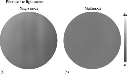
FIGURE 15.5  Phase topographies of an optical flat mirror measured in a Twyman–Green interferometer using phase-stepping interferometry with different fiber types as indicated in the figure. In the case of the single-mode fiber, vertical variations with amplitudes of about ±0.03 interference orders appear.

Parasitic interferences as shown in the earlier example may not appear in general when using single-mode fibers. However, it should be mentioned that their origin could not be identified in the example of Figure 15.5. This means that even when the expected sources of parasitic interferences are switched off (wedged optics, etc.), there still may exist unwanted reflections affecting the measured interference when a spatial coherent light source is used.

15.4.2    GENERATION AND ALIGNMENT OF PLANE WAVES

The realization of the meter in terms of plane electromagnetic waves requires accurate adjustment procedures. A first requirement regards the preparation of the waves itself, that is, the generation of a collimated beam. The collimation of a beam is limited by the divergence of the light source. When laser beams are used directly as a light source, it is recommended to apply a spatial filter for the following reasons: (1) unwanted residual transversal modes of the laser are suppressed effectively, (2) beams can be expanded at the same time, and (3) collimation alignment can easily be adjusted by tuning the position of the second lens of the spatial filter. A wedged shearing plate can be used to generate equally spaced interference fringes in a reflected beam. The beam is collimated properly when the fringes are straight and oriented perpendicular to the wedge orientation. After this adjustment, the divergence of the beam is predetermined by the spatial filter, that is, by the small pinhole size related to the focal length of the second lens acting as a collimator. Instead of observing shearing interferences, the beam profile can be observed and adjusted to be invariant along the propagation direction over a large distance. Alternatively to the usage of spatial filters, the laser may be coupled into an optical fiber, and the fiber output can be set in the focal point position of a collimating lens.

Assuming plane waves; their propagation direction with respect to the direction of the length to be measured must be coincident. Otherwise, as illustrated in Figure 15.6, an angle α causes a cosine error, that is, the length, $\tilde{l}=l\cos \alpha$, is measured to short. In length measurements by interferometry the direction of the collimated beam can be aligned by using an additional mirror in front of the interferometer. Alternatively, when an optical fiber is used as mentioned earlier, the fiber position within the focal plane of the collimator can be adjusted.

In order to adjust the beam direction to be perpendicular to the reflecting faces of a prismatic body, the retroreflected beam is observed in the focal plane of the collimator at the input or at the output of the interferometer. The beam is adjusted in a way that the image of the light source appears exactly in the focal point of the collimator. Such autocollimation adjustment can be realized in different ways. Figure 15.7 illustrates a visual adjustment procedure where the exit pinhole of the interferometer is illuminated via a beam splitter by an additional light source. The light traveling through the pinhole and the collimator lens is reflected by the interferometer mirror and refocused in the focal plane of the collimator forming an image of the pinhole.

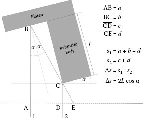
FIGURE 15.6  Derivation of the cosine error. The path difference of the two plane waves reflected at a platen and at the body’s front face is compared with path length 2l.

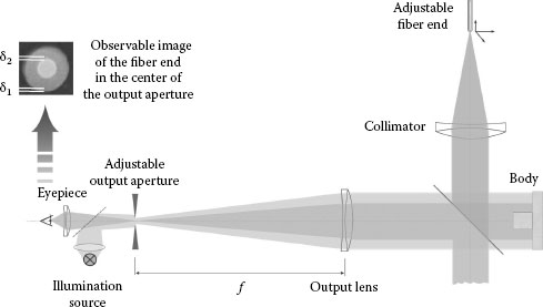
FIGURE 15.7  Visual autocollimation adjustment scheme.

The position of the output pinhole is adjusted so that its image completely coincides with the pinhole. In a second step, the beam direction of the interferometer is adjusted so that the image of the light source, for example, the fiber end, is centered within the exit pinhole. A magnifying lens or microscope is used to observe the pinhole. Although an adequate magnification reduces alignment errors, both procedures are tainted with remaining misalignments indicated by δ₁ and δ₂ in Figure 15.7.

A more direct autocollimation adjustment method is useful when a fiber is used as light source of the interferometer. In this case, the quantity of retroreflected light passing the fiber in reverse direction is observed as shown in Figure 15.8. When this method is combined with scanning in x–y-direction, the resulting signal topography can be used to calculate a center position onto which the fiber end can be positioned more accurately as by the visual method. A further advantage of the retroreflection method is that the collimation can be inspected at the same time, that is, the signal distribution is sensitive to the z-position of the fiber. Misalignment in z-direction leads to a smooth signal distribution, while otherwise a sharp peak appears as indicated in the inset of Figure 15.8.

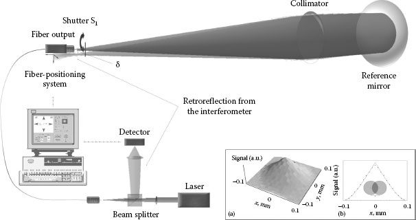
FIGURE 15.8  Scheme of the retroreflection method. The retroreflection signal is detected as a function of the x–y-position of the fiber. The inset shows a measurement example when retroreflection scanning is applied. A section in the x-direction is shown together with a theoretical curve (solid line) obtained from the overlap of two circles representing the fiber and its image.

As mentioned earlier, the size of the light source related to the focal length of the collimator defines the divergence of the collimated beam. This leads to an effect in length measurements by interferometry that was even more important before laser light sources became available but should be taken into consideration further on: the so-called aperture correction can be derived from an integrated cosine error over the light source area. As an example, the aperture correction for a circular light source with diameter d (e.g., a fiber) positioned in the focal point of the collimator amounts to +l (d/4f)², where f is the focal length of the collimator.

A further effect is produced by the finite diameter of the collimated beam. Ideally, plane waves are supposed to propagate between the reflecting surfaces in the interferometer. In reality, the wave fronts are distorted by beam diffraction. For Gaussian beam profiles, the length l to be measured is affected by −l (λ/2πw₀), where w₀ is the beam diameter (waist). As an example, a waist of 3 mm causes an effect of about −1 nm m⁻¹. The size of this effect is even increased by a factor of about 10 when the beam profile is homogeneous. When small beams are used in combination with single detectors, the influence of the beam diffraction entering into the integral interference pattern has to be taken into consideration. Thus, this effect is especially important in compact interferometer designs using small beams, while when expanded beams are used, as in large field imaging interferometers, beam diffraction rings can be ruled out from the interferogram analysis.

15.4.3    DETERMINATION OF THE REFRACTIVE INDEX OF AIR

As already mentioned in Section 15.1, the wavelength in air determines the basic length scale in majority of length measurements performed with interferometry. The wavelength in air results from the vacuum wavelength, λ₀, scaled down with the amount of the refractive index of air:

$\lambda =\frac{{\lambda }_0}{n}.$

(15.3)

Under atmospheric conditions, n is larger by about 2.7 × 10⁻⁴ than unity (vacuum). This deviation, called refractivity, in first-order scales with the atmospheric pressure. Thus, when the atmospheric pressure is determined with a relative uncertainty of 10⁻⁴, which is small, the contribution to the relative uncertainty of the length measurement is still 2.7 × 10⁻⁸ (27 nm m⁻¹). This is larger than three orders of magnitude than the contribution from the uncertainty of the vacuum wavelength of iodine-stabilized laser (≈10^–11). Consequently, n has to be determined highly precisely in interferometric length measurements in air. However, achievement of uncertainty of the air refractive index smaller than 10⁻⁸ is possible only under well-defined laboratory conditions using sophisticated instruments for either measurement of environmental parameters together with appropriate equations or optical refractometers.

The physical background of the air refractive index is based, without going into detail, on the Lorenz–Lorentz equation for the refractive index of a mixture of nonpolar gases:

$\frac{n^2-1}{n^2+2}={\displaystyle \sum _i{R}_i{\text{ρ}}_i},$

(15.4)

where

ρ_i is the partial density of the ith component of the mixture

R_i is the specific refraction, which is invariant to changes of the density to a high degree and which is related to

$R_i=\frac{4}{3}\pi \left(\frac{N_{\text{A}}}{M_i}\right){\alpha }_1,$

(15.5)

where

N_A is the Avogadro constant

M_i is the molecular weight

α_i is the polarizability

For atmospheric air, the dispersion curves for N₂, O₂, and Ar are sufficiently similar. Furthermore, it is assumed in Ciddor’s equation [11] that each CO₂ molecule replaces a molecule of O₂ and that both have the same molecular refractivity so that all these constituents may be combined in a single term on the right-hand side of Equation 15.4. Thus, only water vapor must be treated separately. Finally, the density equation for moist air, for example, the BIPM-1981/91 equation [12], can be used in order to calculate the partial densities in Equation 15.4. Certainly, the use of the density equation requires an accurate measured set of the environmental parameters such as air pressure, temperature, humidity, and CO₂ content.

Alternatively to the earlier-mentioned formalism, there exist a number of empirical equations for the refractive index of air that are called Edlén equations related to one of the scientists suggesting such equation [13]. The basis of these specialized equations are precise measurements of the air refractive index under well-defined laboratory’s standard conditions, that is, these equations are valid exactly under the same standard conditions, only, and may not be used in a wide range of environmental parameters (e.g., in geodetically length measurement) where Ciddor’s equation is mandatory. A valid example for an empirical modified Edlén equation can be found in [14]. Accordingly, the input parameters—wavelength, 633 nm; pressure, 10⁵ Pa; temperature, 20°C; CO₂ content, 400 ppm; relative humidity, 50% (corresponding to a water vapor pressure of 1170 Pa and a dew point of 9.28°C)—lead to a refractive index of n = 1.000267794, which is sensitive to the input parameters as shown in Table 15.1.

The air refractive index may also be obtained directly from using refractometric methods. An example scheme of appropriate refractometer design is shown in Figure 15.9. Here, the optical pathway of light traveled in vacuum is compared with the pathway in air. The vacuum cell can be inserted along the same pathway as used in the length measurement, and for highest accuracy, the same collimated light beam is used as the length measurement path as already indicated in Figure 15.2.

TABLE 15.1
Sensitivity of the Air Refractive Index at Wavelength 633 nm to Changes of Environmental Parameters at Standard Conditions

Influence	Sensitivity	Influence	Sensitivity
Temperature	–9.2E – 07/K	Rel. humidity	–8.7E – 09/%
Pressure	+2.7E – 09/Pa	Dew point	–1.5E – 08/K
CO2 content	+ 1.4E – 10/ppm	Water vapor pressure	–1.8E – 10/Pa

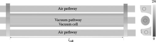
FIGURE 15.9  Scheme of refractometer design using a vacuum cell along the beam pathway of the interferometer. On the right-hand side, a measurement example of phase topography is shown.

In such an approach, the length of the vacuum cell can be written in two alternative ways using Equation 15.1:

$l_{\text{cell}}=\left(i_{\text{vac}}+q_{\text{vac}}\right)\frac{{\lambda }_0}{2}=\left(i_{\text{air}}+q_{\text{air}}\right)\frac{{\lambda }_0}{2n_{\text{air}}},$

(15.6)

in which the subscripts “vac” and “air” indicate the corresponding integer and fractional orders of interference. Using Equation 15.6, the difference between the optical pathways in vacuum and in air can then be written as

$l_{\text{cell}}=\left(n_{\text{air}}-1\right)=\left(\text{Δ}i-\text{Δ}q\right)\frac{{\lambda }_0}{2},$

(15.7)

where

Δi = i_air – i_vac

Δq = q_air – q_vac resulting in

$n_{\text{air}}=\frac{\left(\text{Δ}i-\text{Δ}q\right){\lambda }_0/2}{l_{\text{cell}}}+1.$

(15.8)

The value of Δi may be reversely obtained from Equation 15.7 using an estimate refractive index (e.g., based on environmental parameters using an empirical equation) and setting Δq to zero. Δq results from the interferometric measurement, for example, as indicated on the right-hand side of Figure 15.9, from the interference phase topography:

$\text{Δ}q=\frac{1}{2\pi }\left[\frac{1}{2}\left({\varphi }_{\text{air}}^1+{\varphi }_{\text{air}}^2\right)-{\varphi }_{\text{vac}}\right],$

(15.9)

where

ϕ_vac indicates the mean phase measured within a region of the vacuum pathway

$\frac{1}{2}\left({\varphi }_{\text{air}}^1+{\varphi }_{\text{air}}^2\right)$ is the average of the mean phases in the air pathways in two regions arranged symmetrically around the vacuum pathway

As shown in Figure 15.9, each pathway travels through the transparent plates at both ends of the vacuum cell. These plates should be wedged to avoid parasitic interferences. The wedge angles at both ends should be oriented reversely so that the same pathway through the plates is traveled at each position within the beam’s cross section. However, flatness of the plates and the homogeneity of their refractive index are limited. A way to overcome this limitation can be realized by a correction for the influence of optical pathway differences through the plates. Such so-called zero correction can be extracted from measurements using reconciled vacuum and air pathways, for example, when the interferometer is evacuated together with the vacuum cell, or when the same (dry) gas is injected in the cell as found in the air pathway. In any case, the quality/uncertainty of this correction will limit the attainable measurement uncertainty of the air refractive index using such refractometer. It is noticed that applications of helium gas is a suggested alternative to air environment [15].

15.4.4    IMPORTANCE OF TEMPERATURE MEASUREMENTS

Length measurements are always related to the temperature of the body. For this reason, accurate temperature measurement is very important when length measurements are performed. For example, in primary calibrations of gauge blocks by interferometry, the quantity to be determined is the length at a reference temperature t, mostly 20°C. Typically, during the length measurement by interferometry, the temperature is slightly different from the reference temperature. For this reason, a correction is necessary taking into account the (small) temperature deviation resulting in the length at the reference temperature:

$l_{{20}^{\circ }\text{C}}=l\left[1-{\alpha }_0\left(t-{20}^{\circ }\text{C}\right)\right],$

(15.10)

in which α₀ denotes a constant for the coefficient of thermal expansion. For example, a 1 m gauge block of steel with a typical thermal expansion coefficient of 1.2 × 10⁻⁵ K⁻¹ will be measured about 0.2 µm shorter at t = 19.985°C than at t = 20.000°C. This is even about the half of an interference order and illustrates the importance of accurate temperature measurement. Depending on the body’s material and the desired uncertainty of the length measurement, it may be necessary to perform the temperature measurements with sub-millikelvin uncertainty, traceable to the international temperature scale in its current version [16] as outlined at the BIPM website [17].

In the practical realization of the temperature measurements, it is important to provide a good contact of the calibrated sensors with the body, to account for possible self-heating of the sensors and for temperature gradients along the body.

15.5    INTERFEROMETRY ON PRISMATIC BODIES

While the earlier sections are more of general relevance in length measurements by interferometry, the following sections discuss in detail the special case of length measurements on prismatic bodies, for example, gauge blocks. However, the description is restricted to interferometric techniques in which large field phase-stepping interferometry is combined with imaging onto a camera array. The main advantage of this combination is in well-defined interference phase topographies resulting from the measurements. This provides not only highly accurate length/height topographies but also information about the exact lateral position of a sample body related to the camera array and, therewith, enables accurate length measurements even when the body does not exhibit ideal properties with respect to surface flatness and parallelism. The phase topography at the platen, attached to the body by wringing, may be even used to extract a correction for the flexing of the platen.

It should be mentioned that there exist other length measurement techniques based on interference signals from single detectors. Although such methods may provide a high resolution, the absence of topography and position information increases the attainable uncertainty in these techniques.

15.5.1    IMAGING OF THE BODY ONTO A PIXEL ARRAY

When a prismatic body is set in the measurement pathway of a Twyman–Green interferometer, as shown in Figure 15.1, its length causes a fringe discontinuity at the transition from the body’s front face to the wrung platen. In addition, diffraction occurs at the side edges of the front face. Therefore, in the interfering beams observed at the output of the interferometer, diffraction rings may be observed around the front face. However, when the front face is imaged, which can be achieved by the addition of an appropriate lens in front of the camera, the edges will appear sharp, and the diffraction rings will disappear. This is even more obvious in the phase topography, which can be obtained by applying phase-stepping interferometry. Figure 15.10 illustrates the effect of the aperture size onto the sharpness of the phase topography for a gauge block shaped body in which reflecting front face is particularly textured. In the case of the large aperture of 5 mm (Figure 15.10b), the sharpness is limited by the pixel resolution of the camera, while at 0.5 mm (Figure 15.10c), the sharpness clearly decreases (aperture in the focal point of a lens with f = 700 mm).

Concerning sharpness in the framework of length measurements by interferometry, there are two points to be considered: (1) an aperture is necessary in the focal point of a first lens in the output pathway in order to block unwanted reflections, for example, from the rear side of a wedged beam splitter plate (see Figure 15.1 and the text around), and (2) the image sharpness is reduced when this aperture is undersized. In this case, higher diffraction orders of light deflected at the body’s edges, containing the sharpness information, are blocked as well. Combining (1) and (2), it becomes clear that the distance between secondary spots with respect to the main spot, scaling the maximum possible aperture size, is the limiting parameter for the attainable image sharpness in the interferogram. At a given wedge angle ε, this distance is approximately given by 2εn_BS f, in which n_BS is the refractive index of the beam splitter and f is the focal length of the lens. It is mentioned that in the example of Figure 15.10, the main spot size is 0.2 mm (size of a multimode fiber’s image), while the distance to the secondary spots is 6 mm.

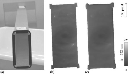
FIGURE 15.10  (a) Photograph of a prismatic body and illustration of image sharpness of the related interference phase topography when the body’s front face is imaged using an appropriate set of lenses and using aperture sizes of (b) 5 mm and (c) 0.5 mm.

The lateral position of a body within the phase topography is important information for the further extraction of the length and, for highest accuracy, length correction related to an average sub-pixel position of the body [18].

15.5.2    INTERFEROGRAM ANALYSIS

Interferogram analysis will give the primary information for further length evaluation, that is, from the measured interferograms, the fractional order of interference is to be extracted as shown in Equation 15.1. This may be done by phase-stepping interferometry as illustrated in Figure 15.11a in which a set of four interferograms each obtained at a different reference pathway is used to calculate a phase topography (Figure 15.11c). Figure 15.11b illustrates the calculation of the phase at a certain pixel position.

Besides interference phase evaluation at each pixel position, it is important to identify the body’s position within the interferogram. When using phase-stepping interferometry, this assignment of the body’s position related to the camera pixel coordinates can be performed most accurately. Different strategies exist for extracting an average sub-pixel-related position of the body. In each case, a tilt between the body’s edges related to the pixel directions of the camera is necessary (as visible in Figure 15.11). One way is to process the discontinuity within the phase topography, which is related to the side edges of the body’s front face. This strategy requires a high quality of the body’s edges surrounding the front face and a nearly perfect right-angled body. Another effective way for extracting an average sub-pixel-related position bases on the use of physical mask pieces that are connected to the front face edges. For gauge block-shaped bodies, the mask may consist of four right-angled metal pieces, which are held in contact against the body’s side edges by a small rubber band as shown in Figure 15.10a. At the pixel positions where these mask pieces are located, no interference is observed. This information can be used to define a mask array in which coordinates of the transitions interference → no interference can be processed around the front face. In Figure 15.11c, these transitions are indicated by black pixels forming lines in a certain range around the front face. In the next step, the coordinates left/right and top/down are averaged resulting in the white pixels forming lines. The coordinates of these pixels are averaged for the two pixel directions separately resulting in a highly accurate sub-pixel coordinate for the central position of the front face. This coordinate is used to define a region of interest (ROI) at the front face and two symmetrically arranged ROIs at the platen, indicated as black squares in Figure 15.11c.

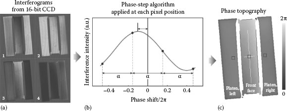
FIGURE 15.11  (a) Set of four interferograms each obtained at a different position of the reference pathway; (b) calculation of the phase value at a certain pixel position using an appropriate phase-stepping algorithm; (c) phase topography obtained from the interferograms: the black pixels around the front face indicate the transitions interference → no interference, the black squares show ROIs in which phase values will be averaged (see text for details).

In principle, the fractional order of interference is based on average phase values within these well-defined ROIs. However, before averaging the phase values, it is necessary to eliminate 2π discontinuities. This procedure is called unwrapping and can easily be performed by processing the phase values within each ROI with respect to phase differences at neighboring pixel positions. The unwrapped phase values may, for example, be obtained from differences by

${\varphi }^{\text{uw}}\left(x,y\right)=\varphi \left(x,y\right)-\text{Round}\left[\varphi \left(x,y\right)-\varphi \left(x-1,y\right)\right].$

(15.11)

Then, the averaged phase values are simply obtained from

${\varphi }_{\text{p}/\text{f}}=\frac{1}{\left(x_{\text{f}}-x_{\text{i}}+1\right)\left(y_{\text{f}}-y_{\text{i}}+1\right)},{\displaystyle \sum _{\underset{y=y_{\text{i}}\dots y_{\text{f}}}{x=x_{\text{i}}\dots x_{\text{f}}}}{\varphi }^{\text{uw}}\left(x,y\right)},$

(15.12)

in which (x_i, y_i) and (x_f, y_f) indicate the initial and final coordinates within each ROI based on the integer of the average position of the body’s front face. For highest accuracy, the exact sub-pixel position of the front face, (x_c, y_c), can be incorporated into the calculation by using

${\varphi }_{\text{p}/\text{f}}=\frac{1}{\left(x_{\text{f}}-x_{\text{i}}+1\right)\left(y_{\text{f}}-y_{\text{i}}+1\right)}{\displaystyle \sum _{\underset{y=y_{\text{i}}\dots y_{\text{f}}}{x=x_{\text{i}}\dots x_{\text{f}}}}{\varphi }^{\text{uw}}\left(x,y\right)+{\varphi }^x\text{Δ}{x}_{\text{c}}+{\varphi }^y\text{Δ}{y}_{\text{c}}}$

(15.13)

instead of Equation 15.12. Here, ϕ^x and ϕ^y indicate the slopes within an ROI along both pixel directions, and the residuals Δx_c = x_c – Round [x_c] and Δy_c = y_c – Round [y_c] take into account for the sub-pixel residuals of the center position of the front face.

It is necessary that the averages within the ROIs on the platen’s left-hand side, ϕ_{p, 1} and on the right-hand side, ϕ_{p, r}, are consistent, that is, approximately within the same plane without 2π discontinuities. Such consistency can be obtained by the so-called left–right unwrapping. In this approach, the average phase on the platen’s left hand is extrapolated to the right-hand side and compared with the actual value on the right-hand side. Then, the integer difference can be used as “unwrapping correction”:

${\varphi }_{\text{p,r}}^{\text{uw}}={\varphi }_{\text{p,r}}-\text{Round}\left[\frac{1}{2\pi }\left({\varphi }_{\text{p,}1}+{\varphi }^x\left(x_{\text{r}}-x_1\right)-{\varphi }_{\text{p},\text{r}}\right)\right],$

(15.14)

where

x_r – x_l is the pixel distance between the ROIs on the left- and right-hand sides

ϕ^x is the average slope along x-direction (left to right) detected within ϕ_{p, 1} and ϕ_{p, r}

From these phase averages, the fractional order of interference can be calculated for each wavelength used in the measurements:

$q=\frac{1}{2\pi }\left[\frac{1}{2}\left({\varphi }_{\text{p,}1}+{\varphi }_{\text{p},\text{r}}^{\text{uw}}\right)-{\varphi }_{\text{f}}\right].$

(15.15)

15.5.3    LENGTH EVALUATION

When the fractional order of interference is provided from the measurements as shown earlier, at a particular wavelength, λ, the body’s length can be expressed as a multiple of the used wavelength, that is, by l = (i + q) λ/2 (Equation 15.1). Consequently, the number of integer interference order i, which is typically large, has to be determined separately to the earlier-described determination of the fractional order q.

When there is only a single wavelength available, the number i must be guessed from Equation 15.1 by setting q = 0:

$i=\text{Round}\left[\frac{l_{\text{est}}}{\left(\lambda /2\right)}\right],$

(15.16)

where l_est is an estimate of the length that can be obtained from the nominal length and the previous knowledge about the deviation δl of the length from the nominal length l_nom. When using only a single wavelength, an error in the determination of i is most likely as, for example, small temperature deviations from the nominal temperature to which l_nom refers (typically 20°C) lead to length changes (see Equation 15.10) that, in most cases, cannot be determined accurately enough. One typical reason for the latter is that the thermal expansion coefficient of a sample body is not known exactly.

When more than one wavelength is available as light source, that is, N different wavelengths, λ_k, k = 1…N, a variation technique referred to as “method of exact fractions” can be used for a more unambiguous extraction of the integer interference orders, i_k, k = 1…N. Moreover, using multiple wavelengths provides the opportunity to check the entire length measurement approach, for example, for correct wavelengths λ_k of the light sources and the correct determination of the fractional interference orders q_k. In this approach, Equation 15.1 represents a set of equations resulting in lengths, which can be compared with each other while the integer orders are varied by whole numbers δ_k, that is, for each wavelength, the length is expressed as

$l_k=\left(i_k+{\delta }_k+q_k\right)\frac{{\lambda }_k}{2},$

(15.17)

in which i_k is calculated from Equation 15.16 for each λ_k. For a set of {δ₁,δ₂,…,δ_N}, the mean length $\overline{l}$ and the amount of average deviations Δ are calculated according to

$\overline{l}=\frac{1}{N}{\displaystyle \sum _{k=1}^N{l}_k},\text{Δ\hspace{0.17em}}=\frac{1}{N}{\displaystyle \sum _{k=1}^N\left|\overline{l}-l_k\right|}.$

(15.18)

The resulting set $\left\{\overline{l},\text{Δ}\right\}$ can be displayed as scatter plot, which represents a coincidence pattern. Figure 15.12 shows a typical example of such pattern in case of two wavelengths (N = 2) in which the data points for Δ < 20 nm are displayed.

In the example shown in Figure 15.12, the two wavelengths are fictively set to λ₁ = 532.3 nm and λ₂ = 548.6 nm. The nominal length is set to l_nom = 10 mm, and the estimate deviation of the length l from the nominal length δl = l − l_nom is set to 2.5 µm. The fractional interference orders q₁ and q₂ are virtually set to q_k = l · 2/λ_k – Round (l · 2/λ_k).

The mentioned input quantities reflect themselves in the coincidence pattern $\left\{\overline{l},\text{Δ}\right\}$ in the following way (see Figure 15.12):

1.  At $\overline{l}-l_{\text{nom}}=\delta l$ , there exists a minimum for which Δ is zero (marked by the dotted circle).

2.  Further minima exist that are spaced by_the half of the so-called synthetic wavelength, λ_synt = λ₁λ₂/(λ₂ – λ₁), that is, at positions $\overline{l}-l_{\text{nom}}=\delta l+m\cdot {\lambda }_{\text{synt}}/2$ in which m is an integer.

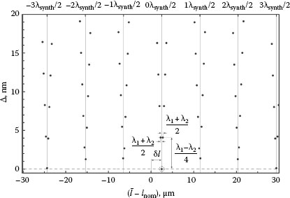
FIGURE 15.12  Typical coincidence pattern when using two wavelengths.

3.  The next neighbored minima for which Δ is zero can be found at specific multiples of λ_synt/2. In this example, the multiples are localized at m = ±3. It is noticed that this number is strongly dependent on the amounts of wavelengths λ₁ and λ₂, that is, there is no rule for a position of these minima.

4.  The lengths that are closest to the minimum $\overline{l}-l_{\text{nom}}=\delta l\left(\text{Δ\hspace{0.17em}}=0\right)$ are separated by a single interference order, that is, at $\overline{l}-l_{\text{nom}}=\delta l\pm \left({\lambda }_1+{\lambda }_2\right)/2$ . The corresponding values of Δ amount to $\left|{\lambda }_1-{\lambda }_2\right|/4$ .

Conclusion (4) reveals a very important requirement for the applicability of the described variation technique: the two wavelengths must be clearly separated. Otherwise, the distance of neighboring lengths mentioned in (4) becomes too small. When, for example, λ₁ and λ₂ would be just 2 nm apart from each other, for {δ₁ ± 1, δ₂ ± l}, the values of Δ result in 0.5 nm, which is very close to zero (zero is obtained for the variation numbers {δ₁, δ₂}). It is noticed for this case that, in spite of the small values of Δ, the corresponding lengths are apart by ±(λ₁ + λ₂)/2!

Conclusion (4) illustrates also that the variation method actually requires “exact fractions.” The “wrong lengths” correlated with {δ₁ ± 1, δ₂ ± l} can be discriminated from the “true lengths” only when l_k can be determined much more accurately than $\left|{\lambda }_1-{\lambda }_2\right|/4$ , that is, when the fractional interference orders (fractions) can be determined “exactly.”

While the earlier example is fictive in order to illustrate the inherent features of the “method of exact fractions,” real measurement examples, even for more than two wavelengths, can be found in the literature (e.g., [19]). Nevertheless, the general conclusion holds for an arbitrary number of wavelengths: the strength of the “method of exact fractions,” that is, the achievable range of unambiguous determination of the integer order of interference, is significantly influenced by the achievable accuracy with which the fractional order of interference can be determined. Moreover, consideration of possible wavelength-dependent effects, for example, phase correction for the surface of the body and chromatic aberration of optical components, might be necessary to be considered.

15.5.4    EXAMPLES OF PRECISE LENGTH MEASUREMENT APPLICATIONS

The first example of length measurements by interferometry focuses on the length measurements separately, that is, influences due to variations of the body’s temperature are minimized by using an ultralow thermal expansion glass as body material. For smallest uncertainty, the measurements were performed under vacuum conditions. The scope of the measurements shown in Figure 15.13 was to investigate the linearity of the interference phase. For this purpose, several measurements were performed at different tilt angles of the reference mirror. The resulting phase topographies are shown as insets in Figure 15.13. The resulting lengths obtained from different measurements are well within 0.1 nm around the mean length of 200,015.19090 µm. Accordingly, nonlinearities of the interference phase could be concluded to be negligible in this example. It is mentioned that autocollimation adjustment was performed as described earlier, that is, in each case, the light beam incidents perpendicular to the body’s faces. The situation is different when the fringes in Figure 15.13 are generated by tilting the body instead of the reference mirror. In such case, the cosine error leads to systematic deviations of several nanometers, dependent on the number of fringes generated (see Section 15.4.2).

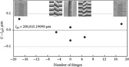
FIGURE 15.13  Length measurements performed at different tilt angles of the reference mirror. The related phase topographies (λ₁ ≅ 532 nm) are shown as insets.

The next example is related to primary length calibrations of long gauge blocks. Here, in addition to the length at a reference temperature, the thermal expansion of a 1 m steel gauge block is investigated by applying a temperature range from 15°C to 25°C. The measurements are performed under atmospheric pressure in a Kösters–Zeiss interference comparator, as shown in Figure 15.2, equipped with phase stepping and a 1 m long vacuum cell dealing as refractometer as outlined in Section 15.4.3. The data points in the lower part of Figure 15.14 show the measured lengths as a function of the temperature. Accordingly, the length varies in a relatively large range around the length at a reference temperature of 20°C (indicated by the zero line). The solid line shows a linear regression fit to the data. Deviations from this linear fit become visible in the middle part of Figure 15.14. The range of these deviations is typical not only for steel material. Applying a second-order fit polynomial to the data results in very small deviations from the fit as shown in the upper part of Figure 15.14.

It is pointed out in this connection that a temperature deviation of only 1 mK leads to a length change of about 12 nm in the 1 m steel gauge block. Accordingly, a very small uncertainty of the temperature measurement is necessary in the example of Figure 15.14. This was achieved by using a sophisticated temperature measurement system with which the surface temperature of the gauge block is transmitted by thermocouples near the front face and near the platen. The advantage of using thermocouples is that self-heating can be neglected. As reference point for the thermocouples, a copper block is used whose temperature is measured by an AC bridge together with a PT-25 standard thermometer. The system is primary calibrated according to ITS90 using the fix points of water and gallium. The temperature measurement uncertainty using the entire calibrated equipment is stated to be 0.5 mK around room temperature.

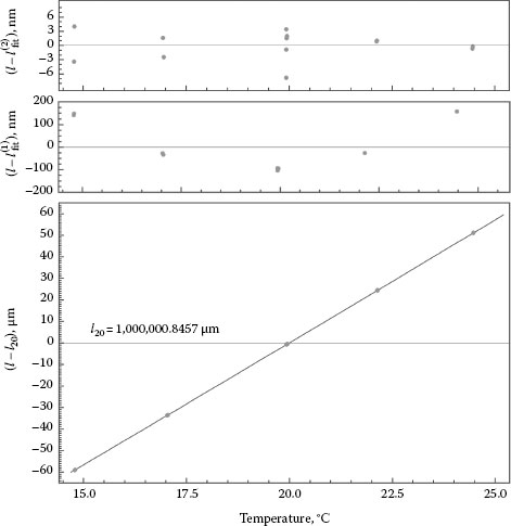
FIGURE 15.14  Length measurements at different temperatures performed on a steel gauge block (data points in the lower part). The solid line shows a linear regression to the data. Deviations from the linear fit and from a second-order polynomial fit become visible in the middle part and in the upper part, respectively.

The second-order polynomial fit, l⁽²⁾, can be used to calculate the coefficient of thermal expansion according to

${\alpha }^{\left(2\right)}\left(t\right)=\frac{1}{l^{\left(2\right)}}\cdot \frac{\text{d}{l}^{\left(2\right)}}{\text{d}t}=\frac{a_1+2a_2\left(t-{20}^{\circ }\text{C}\right)}{a_0+a_1\left(t-{20}^{\circ }\text{C}\right)+a_2{\left(t-{20}^{\circ }\text{C}\right)}^2}\approx \frac{1}{a_0}\left[a_1+2a_2\left(t-{20}^{\circ }\text{C}\right)\right].$

(15.19)

The approximate expression on the right-hand side of Equation 15.18 gives consideration to the fact that the length change is much smaller than the length a₀ = l_20°C itself.

Another example of length measurements at a body made of single-crystal silicon is shown in Figure 15.15. Here, different amounts of air pressure within a Twyman–Green interferometer were set starting from vacuum pressure (10⁻³ hPa). The length of the body is reduced from a value indicated in the figure, with increasing pressure due to the material’s compressibility. The measurements were performed at about 20°C, and the small temperature deviations from 20°C are considered in a correction (Equation 15.10). The overall effect between vacuum and atmospheric pressure is about 65 nm. The straight line shows a linear fit to the data. Except for the vacuum pressure, the pressure was measured by a pressure balance that is difficult to be adjusted at lower pressures (resulting in the larger uncertainties at 250 and 500 hPa as indicated in Figure 15.15). As the silicon crystal is isotropic, the relative length change provides the relative volume change by ΔV/V = 3 · Δl/l. Therefore, the isotropic volume compressibility, K, can be calculated from the slope of the straight line of Figure 15.15 according to

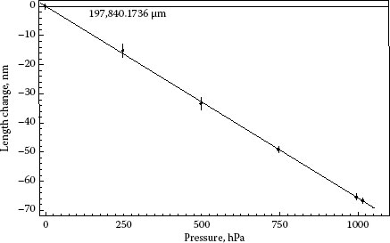
FIGURE 15.15  Length decrease due to the air pressure measured at a body made from single-crystal silicon (data points). Bars indicate the range of measurement uncertainty. The solid line shows a linear regression fit to the data.

$\frac{\text{Δ}l}{l}=-\frac{K}{3}\cdot p,$

(15.19)

in which p is the air pressure within the interferometer.

The next example addresses the so-called length relaxation, which may exist for certain materials but not for single crystals. Length relaxation is observed after the temperature of the material was changed. In contrast to thermal expansion, the temperature of the body may be constant during the length relaxation. In this case, length relaxation can be visualized best. Figure 15.16 shows a measurement cycle performed at a body made of a low-expansion glass ceramics. The initial length (as indicated in the figure) is reduced due to a first stepwise decrease in the temperature toward 10^°C. The inset labeled “10^°C” shows the length relaxation at 10^°C as a function of the time. Residual length relaxation is also visible in the fact that the length at 20°C within the next measurement series toward 30°C (day 10) is smaller than the initial length. The inset labeled “20°C” shows the length relaxation following a single temperature step from 30°C toward 20°C. Accordingly, the length at 20°C is still apart from the initial length even after a period of 10 days. It is pointed out that the functional relationship of the length relaxation is different from a simple exponential course. The solid curves in the insets of Figure 15.16 are of the type

$\text{Δ}l\left(t\right)=c\cdot \exp \left[-{\left(\frac{t}{\tau }\right)}^b\right],$

(15.20)

in which c, τ, and b are fit parameters, whereas the latter was set to 0.5. Equation 15.20 is not sufficient when the length relaxation is to be fit over a longer period of time (data not shown), where a more complex function is necessary.

The long-term stability of materials, shown in the last example, can be regarded as length relaxation over a much longer period of time, initiated by the manufacturing process itself or by any further treatment. However, the long-term behavior of the length is typically described in a time range outside a first relaxation period only. Figure 15.17 shows length measurements performed on two almost identical bodies cut from the same piece of glass ceramics material. The difference between the bodies is that one was heated to 220°C for about 1 h at a time of −0.4 years related to the timescale in Figure 15.17. Accordingly, the heated body exhibits a shrinking that is about fivefold compared to the unheated body, that is, the heat treatment drastically influences the long-term stability, and this effect is visible even after several years.

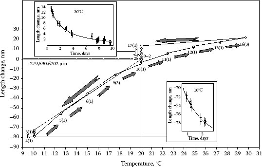
FIGURE 15.16  Length relaxation observed in length measurements by interferometry. Data points indicate the measured length at different positions of the temperature cycle. The insets show the length relaxation at the constant temperatures of 10°C and 20°C, respectively.

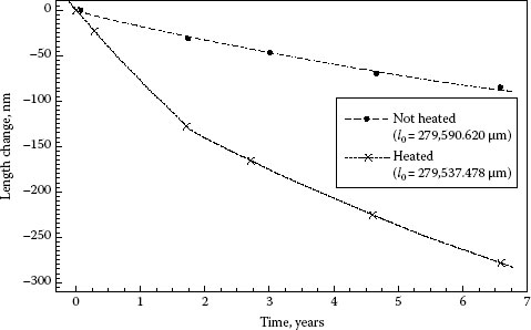
FIGURE 15.17  Length measurements performed on two almost identical bodies cut from the same piece of glass ceramics material: one of the bodies was heated to 220°C for about 1 h at a time of −0.4 years, whereas the other was not heated. In each case, l₀ indicates the length of the body at the first data point (t = 0), and the dashed/dotted lines represent second-order fit polynomials.

15.6    ADDITIONAL CORRECTIONS AND THEIR UNCERTAINTIES

In length measurements by interferometry, it is important to take into account the physical relationship between the interference phase, which is the primary result of the measurements, and the geometrical length to be determined. Some of these points are discussed earlier, for example, the basic idea to relate a body’s length to differences of optical pathways traveled within an interferometer, the direction of the beam, and the size of the light source (aperture correction), as well as the importance of taking into account for the topography of the interference phase by defining appropriate regions of interest within the phase topography.

Besides these points, there are other important aspects that have to be taken into consideration by additional corrections in length measurements by interferometry. Each of these corrections has its uncertainty, which is related to the uncertainty of its determination. On the other hand, each correction’s uncertainty contribution limits the attainable overall combined uncertainty in length measurements by interferometry, which is therefore clearly larger than promised by the interference phase and by the resolution and repeatability of the measurements.

15.6.1    OPTICS ERROR CORRECTION

When an optical flat is inserted in the pathway of an interferometer, normally, a phase topography will be measured that deviates from an ideally plane, even when parasitic interferences are eliminated (see Figure 15.5). In a Twyman–Green interferometer, this deviation still exists when the length of both optical pathways is identical. In this case, deviation of the measured interference topography from an ideal plane represents the sum of optics errors of the interferometer, that is, the imperfectness of the optical components with respect to (1) flatness of optical faces and (2) homogeneity of the optical pathway traveled through the material (including refractive index homogeneity) of the beam splitter (1, 2), compensation plate (2), and the reference mirror (1). An example topography for the optics error of a Twyman–Green interference comparator that is mainly used for primary length calibration of gauge blocks is shown in Figure 15.18. Here, a primary-calibrated optical flat with a maximum flatness deviation of 5 nm is applied. The phase topography was obtained using phase-stepping interferometry from four interferograms measured at a (fourfold) reduced camera resolution of 128 × 128 pixel (x- and y-coordinates) covering the full field of view of about 60 mm in diameter. The data shown in Figure 15.18 are related to a wavelength of 612 nm. Accordingly, the size of deviation from a plane is in the order of 20 nm (according to a phase difference of 0.4 from the side to the center). Averaged values, as displayed by the solid lines along x- and y-directions in the 2D plots of Figure 15.18, are considered as optics error correction for the particular wavelength of 612 nm.

The correction for the optics error of the interferometer can be measured at each of the wavelength used in the measurements. In the interference comparator mentioned earlier, three different wavelengths (612, 633, and 780 nm) are used alternatively. In Figure 15.19, the topographies resulting at different wavelengths are compared by phase differences in which the phases are scaled to each other by the corresponding wavelengths as indicated in the figure. The phase error topographies are consistent within about 0.02 radiant (corresponding to about 1 nm). Accordingly, the measurement uncertainty of the optics error correction at each particular wavelength is limited by the quality of the optical flat used.

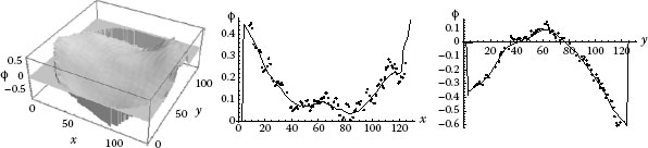
FIGURE 15.18  Phase error due to the interferometer optics measured using an optical flat at a wavelength of 612 nm.

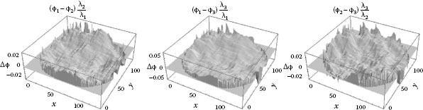
FIGURE 15.19  Consistence check between the optics error corrections obtained at three different wavelengths.

As mentioned earlier, the optics error corrections are measured under the condition that both optical pathways within the interferometer are the same. In this way, wave front errors are excluded. However, in the length measurements, different pathways exist, that is, one at the position of the body’s front face and another at positions of the platen. For this reason, wave front errors are relevant, and there is an effect to the measured phase and, thus, the length. Errors of wave front are not only related to the beam entering the interferometer. In the same way as the wave front of the collimated beam may be distorted, there is an effect due to the interferometer optics. The imperfectness of optical components, which is visible in the optics error correction, causes a wave front distortion as well. To cope with this effect, it is useful to investigate the optics error as described earlier but at different distance levels of the optical flat used. Figure 15.20 shows the difference of phase topographies measured at two positions separated by −100 mm (labeled “top”) and +100 mm (labeled “bottom”) at 612 nm wavelength. Consequently, the difference is up to 0.06 (about 3 nm) and clearly exceeds the differences of the consistence check between the different wavelengths as shown in Figure 15.19.

It is pointed out that the difference shown in Figure 15.20 is clearly influenced by the collimation adjustment of the beam. However, the data shown represent the optimum situation. Consequently, the optics error cannot be corrected completely, but data as shown in Figure 15.20 can be used to estimate an uncertainty of the optics error that is relevant in the length measurements. Certainly, the specific amount of this uncertainty contribution is dependent upon the geometry of the arrangement, that is, definition of the regions of interest within the phase topography. In the example mentioned earlier, it was estimated that the optics error correction is related to an uncertainty contribution of 3 nm, independent of the length of gauge blocks to be calibrated.

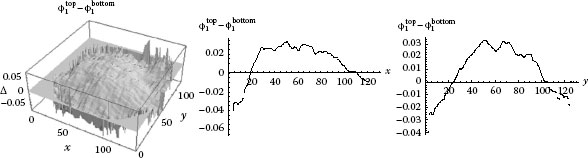
FIGURE 15.20  Difference of phase errors due to the interferometer optics measured at different positions of the optical flat separated by 200 mm (wavelength: 612 nm).

15.6.2    SURFACE ROUGHNESS AND PHASE CHANGE ON REFLECTION

The measured length is affected by the roughness of the surface at which the light is reflected. The effect cancels out in length measurements in which a platen is attached to the body, and both have the same surface roughness. However, this is generally not the case, as, for example, the effect due to surface roughness of steel gauge blocks has been found to vary by several nanometers within a set of gauges. There are a number of techniques for the measurement of surface roughness. One common technique uses an integrating sphere with which light is reflected, and the ratio of the diffuse to directly reflected light is measured. It is assumed that the roughness of a test surface is proportional to the square root of this ratio [20]. This technique requires a calibrated surface, for reference. The roughness difference between a body and a platen is used as correction of the uncertainty, which is typically 3 nm.

There exists another effect to the length measurement that has also to do with the reflection. When light is reflected at normal incidence off the surface of a dielectric material, there is a phase change on reflection, which is π. When the reflecting medium is non-dielectric, that is, there exists absorption loss, the phase change is between 0 and π radians, depending on the properties of the media. In this case, the complex refractive index involves the extinction coefficient κ in addition to the refractive index $n\left(\tilde{n}=n+i\kappa \right)$ . For light traveling in air/vacuum, the phase change on reflection is then given by

$\delta =\text{arctan}\left[\frac{2\kappa }{1-n^2-{\kappa }^2}\right].$

(15.21)

Length-equivalent values for the phase change on reflection are obtained by multiplying half of the wavelength. Typical values for steel are listed in Table 15.2.

Thus, the light beam appears to be reflected approximately 20 nm inside the surface, even if the surface is perfectly smooth. As for roughness, the effect cancels out in length measurements in which a platen is attached to the body, which has the same optical parameters. However, a variation of 4 nm for the length-equivalent difference of the phase change on reflection between the front face and the platen is assumed as uncertainty contribution in primary length calibrations of gauge blocks.

The corrections for the surface roughness and the phase change on reflection are often combined into a single correction termed as “phase correction.”

15.6.3    WRINGING CONTACT BETWEEN A BODY AND A PLATEN

Some length measurement techniques involve a platen to be attached to the body. In this process, often called “wringing,” the surfaces of the body and of the platen are carefully cleaned using a solvent, for example, acetone. When both the surfaces are polished/lapped to the highest degree, they may represent almost perfect optical flats. Putting together enables molecular attraction between the two surfaces, which is much stronger than that needed to hold the weight of the platen. This is also called “optical contacting.” In cases of increased surface roughness when the wringing of completely dry-cleaned surfaces is difficult, a small quantity of wringing fluid may be used, which fills the microscopic gaps. Although, in such a case, the wringing force is somewhat smaller compared to the optical contacting, a so-called wringing film does not contribute to the length as long as the amount of wringing fluid is small.

TABLE 15.2
Typical Parameters for n, κ, and for the Corresponding Length-Equivalent Phase Change on Reflection for Steel

Wavelength (nm)	n	κ	$\frac{\lambda }{2}\delta \left(\text{nm}\right)$
543	2.09	3.00	−19.5
633	2.33	3.21	–20.7
780	2.60	3.54	–22.9

On the other hand, the wringing influences the length measurements by the fact that the surface topography of the body is influenced. This effect is dependent upon any deviation from flatness, mainly of the body’s surface. The difference of length measurements obtained when the platen is wrung to either the one or the other face of the body gives a good indication for this effect. Dependent on the size of the resulting length difference, the wringing influence is considered as uncertainty contribution ranging from 2 to 10 nm for the length measurements.

15.6.4    PLATEN FLEXING

When the length measurement involves a wrung platen that is attached to one of the faces of a prismatic body, the extraction of the length from the interferogram as outlined earlier assumes that the platen represents an ideal flat. Accordingly, the phase on the platen is represented by the mean of averaged unwrapped phase values detected at the platen, for example, by $\frac{1}{2}\left({\varphi }_{\text{p},1}+{\varphi }_{\text{p},\text{r}}^{\text{uw}}\right)$ in Equation 15.15. Platen flexing refers to the deformation of the wrung platen that then cannot be considered as ideal reference plane in the length measurements. There are two ways leading to platen flexing, regardless of the flatness of the isolated platen, both involving the thermal expansion of the material: (1) when, during the wringing, the temperatures of the platen and the body are different, a flexing will be observed after thermal equilibrium; (2) a temperature-dependent platen flexing will be observed when the thermal expansion coefficients of the body and the platen are different. The latter mainly regards thermal expansion measurements extracted from the temperature dependence of the length. The platen’s flexing can be examined from the phase topography. However, there is no direct access to the amount of platen flexing at the center position of the body as the platen’s surface is covered by the body. For this reason, it is useful to extract a flexing correction from the differences in the slopes of unwrapped phases within ROIs on the platen. One suggestion is to assume a parabolic flexing, which leads to a flexing correction for the measured length of

$\delta l_{\text{flexing}}=\frac{\lambda }{2}\frac{1}{2\pi }\left(\frac{\partial {\varphi }_{\text{Pr}}}{\partial x}-\frac{\partial {\varphi }_{\text{Pl}}}{\partial x}\right)\frac{x_{\text{r}}-x_1}{4},$

(15.22)

in which x_r – x_l represents the distance between the ROIs located at the platen. The uncertainty of the flexing correction is dependent on the accuracy of the phase topography and the size and geometry of the ROIs. Uncertainties of up to 0.1 nm could be achieved for the standard design of gauge block-shaped bodies, that is, for l × 35 mm × 9 mm.

15.7    CONCLUSIONS

This chapter describes the principles of highest-level length measurements by optical interferometry. The main focus is on measurements in which the length of a body is represented by a step height, which allows measurement by probing in one direction. This is advantageous because the penetration of the probe into the surface of the body and platen due to phase effects is then accounted for when the platen and body are of the same material.

The main conclusion of this chapter is that length measurements by interferometry, which provide the link between the lengths of macroscopic bodies to the SI-definition of the meter, can be performed highly accurately when the light waves and their alignment are provided on a very high level. Under certain conditions where additional phase corrections can be regarded as constant, for example, in thermal expansion or stability measurements of materials, the length measurements can be performed with even sub-nanometer uncertainty. However, in the general case of length measurements by interferometry, the attainable uncertainty is clearly larger than 10⁻⁸l. This can be due to limited uncertainty of the temperature measurement but mainly due to necessary corrections, which must be considered carefully and which comprise their uncertainty contributions. The situation is the same even if picometer resolution or repeatability is achieved in the measurements.

REFERENCES

1.  Unit of length (metre), SI brochure, Section 2.1.1.1. URL: http://www.bipm.org/en/si/si_brochure/chapter2/2-1/metre.html (accessed August 24, 2013).

2.  H. Haitjema. Achieving traceability and sub-nanometer uncertainty using interferometric techniques. Meas. Sci. Technol. 19 (2008) 084002.

3.  J. H. Bruning, D. R. Herriott, J. E. Gallagher, D. P. Rosenfeld, A. D. White, and D. J. Brangaccio. Digital wave-front measuring interferometer for testing optical surfaces and lenses. Appl. Opt. 13 (1974) 2693–2703.

4.  K. Creath. Step height measurement using two-wavelength phase-shifting interferometry. Appl. Opt. 26 (1987) 2810–2816.

5.  G. Bönsch. Gauge blocks as length standards measured by interferometry or comparison length definition, traceability chain and limitations. Proc. SPIE 3477 (1998) 199–210.

6.  J. E. Decker, R. Schödel, and G. Bönsch. Next generation Kösters interferometer. Proc. SPIE 5190 (2003) 14–23.

7.  G. Bönsch and H. Böhme. Phase-determination of Fizeau interferences by phaseshifting interferometry. Optik 82 (1989) 161–164.

8.  J. B. Saunders, Sr. Ball and cylinder interferometer. J. Res. Nat. Bur. Stand. 76C (1972) 11–20.

9.  R. A. Nicolaus and G. Bönsch. A novel interferometer for dimensional measurement of a silicon sphere. IEEE Trans. Instrum. Meas. 46 (1997) 563–565.

10.  C. Weichert, P. Köchert, R. Köning, J. Flügge, B. Andreas, U. Kuetgens, and A. Yacoot. A heterodyne interferometer with periodic nonlinearities smaller than ± 10 pm. Meas. Sci. Technol. 23 094005 (2012).

11.  P. E. Ciddor. Refractive index of air: New equations for the visible and near infrared. Appl. Opt. 35 (1996) 1566–1573.

12.  R. S. Davis. Equation for the determination of the density of moist air. (1981/91) Metrologia 29 (1992) 67–70.

13.  B. Edlén. The refractive index of air. Metrologia 2 (1966) 71–80.

14.  G. Bönsch and E. Potulski. Measurement of the refractive index of air and comparison with modified Edlen’s formulae. Metrologia 35 (1998) 133–139.

15.  J. A. Stone and A. Stejskal. Using helium as a standard of refractive index: Correcting errors in a gas refractometer. Metrologia 41 (2004) 189–197.

16.  H. Preston-Thomas. The International Temperature Scale of 1990 (ITS-90). Metrologia 77 (1990) 3–10.

17.  Unit of thermodynamic temperature (kelvin), SI brochure, Section 2.1.1.5 URL: http://www.bipm.org/en/si/si_brochure/chapter2/2-1/kelvin.html (accessed August 24, 2013).

18.  R. Schödel. Compensation of wavelength dependent image shifts in imaging optical interferometry. Appl. Opt. 46 (2007) 7464–7468.

19.  R. Schödel. Ultra high accuracy thermal expansion measurements with PTB’s precision interferometer. Meas. Sci. Technol. 19 (2008) 084003.

20.  G. Bönsch. Interferometric calibration of an integrating sphere for determination of the roughness correction of gauge blocks. Proc. SPIE 3477 (1998) 152–160.