
Chapter 10. Physical Layer Overview
Any girl can be glamorous.
All you have to do is stand still and look stupid.
— Hedy Lamarr
Protocol layering allows for research, experimentation, and improvement on different parts of the protocol stack. The second major component of the 802.11 architecture is the physical layer, which is often abbreviated PHY. This chapter introduces the common themes and techniques that appear in each of the radio-based physical layers and describes the problems common to all radio-based physical layers; it is followed by more detailed explanations of each of the physical layers that are standardized for 802.11.
Physical-Layer Architecture
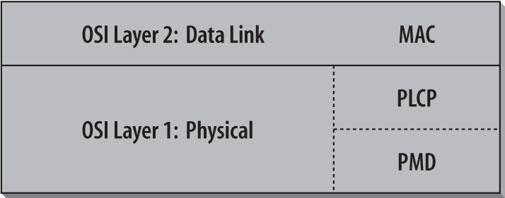
The physical layer is divided into two sublayers: the Physical Layer Convergence Procedure (PLCP) sublayer and the Physical Medium Dependent (PMD) sublayer. The PLCP (Figure 10-1) is the glue between the frames of the MAC and the radio transmissions in the air. It adds its own header. Normally, frames include a preamble to help synchronize incoming transmissions. The requirements of the preamble may depend on the modulation method, however, so the PLCP adds its own header to any transmitted frames. The PMD is responsible for transmitting any bits it receives from the PLCP into the air using the antenna. The physical layer also incorporates a clear channel assessment (CCA) function to indicate to the MAC when a signal is detected.
The Radio Link
Three physical layers were standardized in the initial revision of 802.11, which was published in 1997:
Later, three further physical layers based on radio technology were developed:
802.11a: Orthogonal Frequency Division Multiplexing (OFDM) PHY
802.11b: High-Rate Direct Sequence (HR/DS or HR/DSSS) PHY
802.11g: Extended Rate PHY (ERP)
The future 802.11n, which is colloquially called the MIMO PHY or the High-Throughput PHY
This book discusses the physical layers based on radio waves in detail; it does not discuss the infrared physical layer, which to my knowledge has never been implemented in a commercial product.
Licensing and Regulation
The classic approach to radio communications is to confine an information-carrying signal to a narrow frequency band and pump as much power as possible (or legally allowed) into the signal. Noise is simply the naturally present distortion in the frequency band. Transmitting a signal in the face of noise relies on brute force—you simply ensure that the power of the transmitted signal is much greater than the noise.
In the classic transmission model, avoiding interference is a matter of law, not physics. With high power output in narrow bands, a legal authority must impose rules on how the RF spectrum is used. In the United States, the Federal Communications Commission (FCC) is responsible for regulating the use of the RF spectrum. Many FCC rules are adopted by other countries throughout the Americas. European allocation is performed by the European Radiocommunications Office (ERO) and the European Telecommunications Standards Institute (ETSI). In Japan, the Ministry of Internal Communications (MIC) regulates radio usage. Worldwide “harmonization” work is often done under the auspices of the International Telecommunications Union (ITU). Many national regulators will adopt ITU recommendations.
For the most part, an institution must have a license to transmit at a given frequency. Licenses can restrict the frequencies and transmission power used, as well as the area over which radio signals can be transmitted. For example, radio broadcast stations must have a license from the FCC. Likewise, mobile telephone networks must obtain licenses to use the radio spectrum in a given market. Licensing guarantees the exclusive use of a particular set of frequencies. When licensed signals are interfered with, the license holder can demand that a regulatory authority step in and resolve the problem, usually by shutting down the source of interference. Intentional interference is equivalent to trespassing, and may be subject to criminal or civil penalties.
Frequency allocation and unlicensed frequency bands
Radio spectrum is allocated in bands dedicated to a particular purpose. A band defines the frequencies that a particular application may use. It often includes guard bands, which are unused portions of the overall allocation that prevent extraneous leakage from the licensed transmission from affecting another allocated band.
Several bands have been reserved for unlicensed use. For example, microwave ovens operate at 2.45 GHz, but there is little sense in requiring homeowners to obtain permission from the FCC to operate microwave ovens in the home. To allow consumer markets to develop around devices built for home use, the FCC (and its counterparts in other countries) designated certain bands for the use of “industrial, scientific, and medical” equipment. These frequency bands are commonly referred to as the ISM bands. The 2.4-GHz band is available worldwide for unlicensed use.[47] Unlicensed use, however, is not the same as unlicensed sale. Building, manufacturing, and designing 802.11 equipment does require a license; every 802.11 card legally sold in the U.S. carries an FCC identification number. The licensing process requires the manufacturer to file a fair amount of information with the FCC. Much this information is a matter of public record and can be looked up online by using the FCC identification number.
Use of equipment in the ISM bands is generally license-free, provided that devices operating in them do not emit significant amounts of radiation. Microwave ovens are high-powered devices, but they have extensive shielding to restrict radio emissions. Unlicensed bands have seen a great deal of activity in the past three years as new communications technologies have been developed to exploit the unlicensed band. Users can deploy new devices that operate in the ISM bands without going through any licensing procedure, and manufacturers do not need to be familiar with the licensing procedures and requirements. At the time this book was written, a number of new communications systems were being developed for the 2.4-GHz ISM band:
The variants of 802.11 that operate in the band (the frequency-hopping layer, both direct sequence layers, and the OFDM layer)
Bluetooth, a short-range wireless communications protocol developed by an industry consortium led by Ericsson
Spread-spectrum cordless phones introduced by several cordless phone manufacturers
X10, a protocol used in home automation equipment that can use the ISM band for video transmission
Unfortunately, “unlicensed” does not necessarily mean “plays well with others.” All that unlicensed devices must do is obey limitations on transmitted power. No regulations specify coding or modulation, so it is not difficult for different vendors to use the spectrum in incompatible ways. As a user, the only way to resolve this problem is to stop using one of the devices; because the devices are unlicensed, regulatory authorities will not step in.
Other unlicensed bands
Additional spectrum is available in the 5 GHz range. The United States was the first country to allow unlicensed device use in the 5 GHz range, though both Japan and Europe followed.[48] There is a large swath of spectrum available in various countries around the world:
4.92-4.98 GHz (Japan)
5.04-5.08 GHz (Japan)
5.15-5.25 GHz (United States, Japan)
5.25-5.35 GHz (United States)
5.47-5.725 GHz (United States, Europe)
5.725-5.825 GHz (United States)
Devices operating in 5 GHz range must obey limitations on channel width and radiated power, but no further constraints are imposed. Japanese regulations specify narrower channels than either the U.S. or Europe.
Spread Spectrum
Spread-spectrum technology is the foundation used to reclaim the ISM bands for data use. Traditional radio communications focus on cramming as much signal as possible into as narrow a band as possible. Spread spectrum works by using mathematical functions to diffuse signal power over a large range of frequencies. When the receiver performs the inverse operation, the smeared-out signal is reconstituted as a narrow-band signal, and, more importantly, any narrow-band noise is smeared out so the signal shines through clearly.
Use of spread-spectrum technologies is a requirement for unlicensed devices. In some cases, it is a requirement imposed by the regulatory authorities; in other cases, it is the only practical way to meet regulatory requirements. As an example, the FCC requires that devices in the ISM band use spread-spectrum transmission and impose acceptable ranges on several parameters.
Spreading the transmission over a wide band makes transmissions look like noise to a traditional narrowband receiver. Some vendors of spread-spectrum devices claim that the spreading adds security because narrowband receivers cannot be used to pick up the full signal. Any standardized spread-spectrum receiver can easily be used, though, so additional security measures are mandatory in nearly all environments.
This does not mean that spread spectrum is a “magic bullet” that eliminates interference problems. Spread-spectrum devices can interfere with other communications systems, as well as with each other; and traditional narrow-spectrum RF devices can interfere with spread spectrum. Although spread spectrum does a better job of dealing with interference within other modulation techniques, it doesn’t make the problem go away. As more RF devices (spread-spectrum or otherwise) occupy the area that your wireless network covers, you’ll see the noise level go up, the signal-to-noise ratio decrease, and the range over which you can reliably communicate drop.
To minimize interference between unlicenced devices, the FCC imposes limitations on the power of spread-spectrum transmissions. The legal limits are one watt of transmitter output power and four watts of effective radiated power (ERP). Four watts of ERP are equivalent to 1 watt with an antenna system that has 6-dB gain, or 500 milliwatts with an antenna of 10-dB gain, etc.[49] The transmitters and antennas in PC Cards are obviously well within those limits—and you’re not getting close even if you use a commercial antenna. But it is possible to cover larger areas by using an external amplifier and a higher-gain antenna. There’s no fundamental problem with doing this, but you must make sure that you stay within the FCC’s power regulations.
Types of spread spectrum
The radio-based physical layers in 802.11 use three different spread-spectrum techniques:
- Frequency hopping (FH or FHSS)
Frequency-hopping systems jump from one frequency to another in a random pattern, transmitting a short burst at each subchannel. The 2-Mbps FH PHY is specified in clause 14.
- Direct sequence (DS or DSSS)
Direct-sequence systems spread the power out over a wider frequency band using mathematical coding functions. Two direct-sequence layers were specified. The initial specification in clause 15 standardized a 2-Mbps PHY, and 802.11b added clause 18 for the HR/DSSS PHY.
- Orthogonal Frequency Division Multiplexing (OFDM)
OFDM divides an available channel into several subchannels and encodes a portion of the signal across each subchannel in parallel. The technique is similar to the Discrete Multi-Tone (DMT) technique used by some DSL modems. Clause 17, added with 802.11a, specifies the OFDM PHY. Clause 18, added in 802.11g, specifies the ERP PHY, which is essentially the same but operating at a lower frequency.
Frequency-hopping systems are the cheapest to make. Precise timing is needed to control the frequency hops, but sophisticated signal processing is not required to extract the bit stream from the radio signal. Direct-sequence systems require more sophisticated signal processing, which translates into more specialized hardware and higher electrical power consumption. Direct-sequence techniques also allow a higher data rate than frequency-hopping systems.
RF Propagation with 802.11
In fixed networks, signals are confined to wire pathways, so network engineers do not need to know anything about the physics of electrical signal propagation. Instead, there are a few rules used to calculate maximum cable length, and as long as the rules are obeyed, problems are rare. RF propagation is not anywhere near as simple.
Signal Reception and Performance
Space is full of random electromagnetic waves, which can easily be heard by tuning a radio to an unused frequency. Radio communication depends on making a signal intelligible over the background noise. As conditions for reception degrade, the signal gets closer to the noise floor. Performance is determined largely by the the most important factor, the signal-to-noise ratio (SNR). In Figure 10-2, the SNR is illustrated by the height of the peak of the signal above the noise floor.

Having a strong signal is important, but not the whole story. Strong signals can be hard to pick out of noisy environments. In some situations, it may be possible to raise the power to compensate for a high noise floor. Unlicensed networks have only limited ability to raise power because of tight regulatory constraints. As a result, more effort is placed on introducing as little additional noise as possible before attempting to decode the radio signal.
The Shannon limit
Interestingly enough, there is no theoretical maximum to the amount of data that can be carried by a radio channel. The capacity of a communications channel is given by the Shannon-Hartley theorem, which was proved by Bell Labs researcher Claude Shannon in 1948. The theorem expresses the mathematical limit of the capacity of a communications channel, which is named after the theorem and is often called the Shannon limit or the Shannon capacity. The original Shannon theorem expressed the maximum capacity C bits per second as a function of the bandwidth W in Hertz, and the absolute ratio of signal power to noise. If the gain is measured in decibels, simply solve the equation that defines a decibel for the power ratio for the second form.
Figure 10-3 shows the Shannon limit as a function of the signal-to-noise ratio. Shannon’s theorem reflects a theoretical reality of an unlimited bit rate. To get to an unlimited bit rate, the code designer can require an arbitrarily large number of signal levels to distinguish between bits, but the fine distinctions between the arbitrarily close signal rates will be swamped by the noise. One of the major goals for 802.11 PHY designers is to design encoding rates as close to the Shannon limit as possible.
Alternatively, the Shannon theorem can be used to prescribe the minimum theoretical signal to noise ratio to attain a given data rate. Solve the previous equations for the signal to noise ratio:
| S/N = 2 ^ (C/W) - 1 (S/N as power ratio) |
| SNR = 10 * log10 (2 ^ (C/W) - 1) (SNR as dB) |
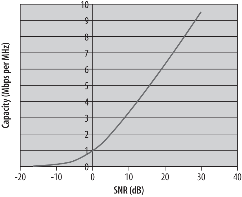
Take 802.11a as an example. A single 20 MHz channel can carry a signal at a data rate up to 54 Mbps. Solving for the required signal-to-noise ratio yields 7.4 dB, which is much lower than what is required by most real products on the market, reflecting the need of products to work in the real-world with much worse than ideal performance.[50]
Path Loss, Range, and Throughput
In 802.11, the speed of the network depends on range. Several modulation types are defined by the various 802.11 standards, ranging in speed from 1 Mbps to 54 Mbps. Receiver circuits must distinguish between states to extract bits from radio waves. Higher speed modulations pack more bits into a given time interval, and require a cleaner signal (and thus higher signal-to-noise ratio) to successfully decode.
As radio signals travel through space, they degrade. For the most part, the noise floor will be relatively constant over the limited range of an 802.11 network. Over distance, the degradation of the signal will limit the signal-to-noise ratio at the receiver. As a station strays farther from an access point, the signal level drops; with a constant noise floor, the degraded signal will result in a degraded signal to noise ratio. Figure 10-4 illustrates this concept. As range from the access point increases, the received signal gets closer to the noise floor. Stations that are closer have higher signal to noise ratios. As a matter of network engineering, when the signal-to-noise ratio gets too small to support a high data rate, the station will fall back to a lower data rate with less demanding signal-to-noise ratio requirements.

When there are no obstacles to obstruct the radio wave, the signal degradation can be calculated with the following equation. The loss in free-space is sometimes called the path loss because it is the minimum loss that would be expected along a path with a given length. Path loss depends on the distance and the frequency of the radio wave. Higher distances and higher frequencies lead to higher path loss. One reason why 802.11a has shorter range than 802.11b and 802.11g is that the path loss is much higher at the 5 GHz used by 802.11a. The equation for free-space path loss is:
| Path loss (dB) = 32.5 + 20 log F + 20 log d |
where the frequency F is expressed in GHz, and the distance d is expressed in meters. Path loss is not, however, the only determinant of range. Obstacles such as walls and windows will reduce the signal, and antennas and amplifiers may be used to boost the signal, which compensates for transmission losses. Range calculations often include a fudge factor called the link margin to account for unforeseen losses.
| Total loss = TX power + TX antenna gain - path loss - obstacle loss - link margin + RX antenna gain |
Multipath Interference
Although there is a relatively simple equation for predicting radio propagation, it is only an estimate for 802.11 networks. In addition to straight-line path losses, there are other phenomena that can inhibit signal reception with 802.11. One of the major problems that plague radio networks is multipath fading. Waves are added by superposition. When multiple waves converge on a point, the total wave is simply the sum of any component waves. Figure 10-5 shows a few examples of superposition.

In Figure 10-5 (c), the two waves are almost exactly the opposite of each other, so the net result is almost nothing. Unfortunately, this result is more common than you might expect in wireless networks. Most 802.11 equipment uses omnidirectional antennas, so RF energy is radiated in every direction. Waves spread outward from the transmitting antenna in all directions and are reflected by surfaces in the area. Figure 10-6 shows a highly simplified example of two stations in a rectangular area with no obstructions.

This figure shows three paths from the transmitter to the receiver. The wave at the receiver is the sum of all the different components. It is certainly possible that the paths shown in Figure 10-6 will all combine to give a net wave of 0, in which case the receiver will not understand the transmission because there is no transmission to be received.
Because the interference is a delayed copy of the same transmission on a different path, the phenomenon is called multipath fading or multipath interference. In many cases, multipath interference can be resolved by changing the orientation or position of the receiver.
Inter-Symbol Interference (ISI)
Multipath fading is a special case of inter-symbol interference. Waves that take different paths from the transmitter to the receiver will travel different distances and be delayed with respect to each other, as in Figure 10-7. Once again, the two waves combine by superposition, but the effect is that the total waveform is garbled. In real-world situations, wavefronts from multiple paths may be added. The time between the arrival of the first wavefront and the last multipath echo is called the delay spread. Longer delay spreads require more conservative coding mechanisms. 802.11b networks can handle delay spreads of up to 500 ns, but performance is much better when the delay spread is lower. When the delay spread is large, many cards will reduce the transmission rate; several vendors claim that a 65-ns delay spread is required for full-speed 11-Mbps performance at a reasonable frame error rate. (Discussion of reading the specification sheets is found in Chapter 16.) Analysis tools can be used to measure the delay spread.

RF Engineering for 802.11
802.11 has been adopted at a stunning rate. Many network engineers accustomed to signals flowing along well-defined cable paths are now faced with a LAN that runs over a noisy, error-prone, quirky radio link. In data networking, the success of 802.11 has inexorably linked it with RF engineering. A true introduction to RF engineering requires at least one book, and probably several. For the limited purposes I have in mind, the massive topic of RF engineering can be divided into two parts: how to make radio waves and how radio waves move.
RF Components
RF systems complement wired networks by extending them. Different components may be used depending on the frequency and the distance that signals are required to reach, but all systems are fundamentally the same and made from a relatively small number of distinct pieces. Two RF components are of particular interest to 802.11 users: antennas and amplifiers. Antennas are of general interest since they are the most tangible feature of an RF system. Amplifiers complement antennas by allowing the antennas to pump out more power, which may be of interest depending on the type of 802.11 network you are building.
Antennas
Antennas are the most critical component of any RF system because they convert electrical signals on wires into radio waves and vice versa. In block diagrams, antennas are usually represented by a triangular shape, as shown in Figure 10-8.

To function at all, an antenna must be made of conducting material. Radio waves hitting an antenna cause electrons to flow in the conductor and create a current. Likewise, applying a current to an antenna creates an electric field around the antenna. As the current to the antenna changes, so does the electric field. A changing electric field causes a magnetic field, and the wave is off.
The size of the antenna you need depends on the frequency: the higher the frequency, the smaller the antenna. The shortest simple antenna you can make at any frequency is 1/2 wavelength long (although antenna engineers can play tricks to reduce antenna size further). This rule of thumb accounts for the huge size of radio broadcast antennas and the small size of mobile phones. An AM station broadcasting at 830 kHz has a wavelength of about 360 meters and a correspondingly large antenna, but an 802.11b network interface operating in the 2.4-GHz band has a wavelength of just 12.5 centimeters. With some engineering tricks, an antenna can be incorporated into a PC Card or around the laptop LCD screen, and a more effective external antenna can easily be carried in a backpack or computer bag.
Antennas can also be designed with directional preference. Many antennas are omnidirectional, which means they send and receive signals from any direction. Some applications may benefit from directional antennas, which radiate and receive on a narrower portion of the field. Figure 10-9 compares the radiated power of omnidirectional and directional antennas.

For a given amount of input power, a directional antenna can reach farther with a clearer signal. They also have much higher sensitivity to radio signals in the dominant direction. When wireless links are used to replace wireline networks, directional antennas are often used. Mobile telephone network operators also use directional antennas when cells are subdivided. 802.11 networks typically use omnidirectional antennas for both ends of the connection, although there are exceptions—particularly if you want the network to span a longer distance. Also, keep in mind that there is no such thing as a truly omnidirectional antenna. We’re accustomed to thinking of vertically mounted antennas as omnidirectional because the signal doesn’t vary significantly as you travel around the antenna in a horizontal plane. But if you look at the signal radiated vertically (i.e., up or down) from the antenna, you’ll find that it’s a different story. And that part of the story can become important if you’re building a network for a college or corporate campus and want to locate antennas on the top floors of your buildings.
Of all the components presented in this section, antennas are the most likely to be separated from the rest of the electronics. In this case, you need a transmission line (some kind of cable) between the antenna and the transceiver. Transmission lines usually have an impedance of 50 ohms.
In terms of practical antennas for 802.11 devices in the 2.4-GHz band, the typical wireless PC Card has an antenna built in. Built-in antennas work, but they will never be anything to write home about. At best, the built in antenna in a PC card is mediocre. Larger antennas perform better. Some PC Card 802.11 interfaces have external antenna jacks. With an optional external antenna, the card has better performance, at the cost of aesthetic quality. In response to the need for improved antenna performance without ugly space-consuming external antennas, many laptops now use an antenna built into the frame around the laptop screen.
Amplifiers
Amplifiers make signals bigger. Signal boost, or gain, is measured in decibels (dB). Amplifiers can be broadly classified into three categories: low-noise, high-power, and everything else. Low-noise amplifiers (LNAs) are usually connected to an antenna to boost the received signal to a level that is recognizable by the electronics the RF system is connected to. LNAs are also rated for noise factor, which is the measure of how much extraneous information the amplifier introduces. Smaller noise factors allow the receiver to hear smaller signals and thus allow for a greater range.
High-power amplifiers (HPAs) are used to boost a signal to the maximum power possible before transmission. Output power is measured in dBm, which are related to watts (see the "Decibels and Signal Strength" sidebar earlier in this chapter). Amplifiers are subject to the laws of thermodynamics, so they give off heat in addition to amplifying the signal. The transmitter in an 802.11 PC Card is necessarily low-power because it needs to run off a battery if it’s installed in a laptop, but it’s possible to install an external amplifier at fixed access points, which can be connected to the power grid where power is more plentiful.
This is where things can get tricky with respect to compliance with regulations. 802.11 devices are limited to one watt of power output and four watts effective radiated power (ERP). ERP multiplies the transmitter’s power output by the gain of the antenna minus the loss in the transmission line. So if you have a 1-watt amplifier, an antenna that gives you 8 dB of gain, and 2 dB of transmission line loss, you have an ERP of 4 watts; the total system gain is 6 dB, which multiplies the transmitter’s power by a factor of 4.
[47] The 2.4-GHz ISM band is reserved by the FCC rules (Title 47 of the Code of Federal Regulations), part 15.247. ETSI reserved the same spectrum in ETSI Technical Specifications (ETS) 300-328.
[48] Europe is obviously not a single country, but there is a European-wide spectrum regulator.
[49] Remember that the transmission line is part of the antenna system, and the system gain includes transmission line losses. So an antenna with 7.5-dB gain and a transmission line with 1.5-dB loss has an overall system gain of 6 dB. It’s worth noting that transmission line losses at UHF frequencies are often very high; as a result, you should keep your amplifier as close to the antenna as possible.
[50] Or, as another example, the telephone network makes channels with a frequency band of 180 Hz to 3.2 kHz, at a signal-to-noise ratio of 45 dB. That makes the maximum theoretical speed of an analog signal about 45 kbps. The trick behind the 56 kbps modem is that the downstream path is all digital, and as a result has a higher signal-to-noise ratio.