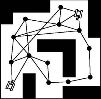
The first step in pathfinding is to define the search area. We need some way to represent the game world in a manner that allows the search algorithm to search for and find the best path. Ultimately, the game world needs to be represented by points that both the game characters and objects can occupy. It is the pathfinding algorithm’s job to find the best path between any two points, avoiding any obstacles. How the actual game world will be represented depends on the type of game. In some cases, the game world might have to be simplified. For example, a game which uses a continuous environment would probably be made up of a very large number of points that the game characters would be able to occupy. The A∗ algorithm would not be practical for this type of search space. It simply would be too large. However, it might work if the search area could be simplified. This would involve placing nodes throughout the game world. We then would be able to build paths between nodes, but not necessarily between every possible point in the world. This is illustrated in Figure 7-1.

Figure 7-1. Simplifying the search area

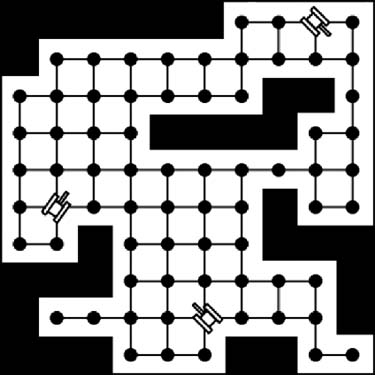
The tanks in Figure 7-1 are free to occupy any point in their coordinate system, but for the purposes of pathfinding, the game world is simplified by placing nodes throughout the game environment. These nodes do not correspond directly to every possible tank position. That would require too many nodes. We need to reduce the nodes to a manageable number, which is what we mean when we say we need to simplify the search area.

Of course, we need to maintain a list of the connections between the nodes. The search algorithm needs to know how the nodes connect. Once it knows how they link together, the A∗ algorithm can calculate a path from any node to any other node. The more nodes placed in the world, the slower the pathfinding process. If pathfinding is taking too many CPU cycles, one alternative is to simplify the search area by using fewer nodes.

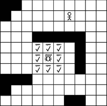
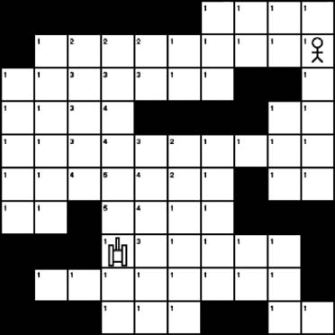
On the other hand, a game that uses a tiled world would be a good candidate for the A∗ algorithm, assuming, of course, that the world isn’t unreasonably large. It would be a good candidate because essentially the world already would be divided into nodes. Each tile would be a node in the search area. This is illustrated in Figure 7-2.

Figure 7-2. Tiled search area

Tiled environments, such as the one shown in Figure 7-2, are well suited to the A∗ algorithm. Each tile serves as a node in the search area. You don’t need to maintain a list of links between the nodes because they are already adjacent in the game world. If necessary, you also can simplify tiled environments. You can place a single node to cover multiple tiles. In the case of very large tiled environments, you can set up the pathfinding algorithm to search only a subset of the world. Think of it as a smaller square within a larger square. If a path cannot be found within the confines of the smaller square, you can assume that no reasonable path exists.

Once we have simplified the search area so that it’s made up of a reasonable number of nodes, we are ready to begin the search. We will use the A∗ algorithm to find the shortest path between any two nodes. In this example, we will use a small tiled environment. Each tile will be a node in the search area and some nodes will contain obstacles. We will use the A∗ algorithm to find the shortest path while avoiding the obstacles. Example 7-1 shows the basic algorithm we will follow.

add the starting node to the open list
while the open list is not empty
   {
      current node=node from open list with the lowest cost
      if current node = goal node then
          path complete
      else
          move current node to the closed list
          examine each node adjacent to the current node
          for each adjacent node
            if it isn't on the open list
               and isn't on the closed list
                  and it isn't an obstacle then
                     move it to open list and calculate cost
   }

Some of the particulars of the pseudo code shown in Example 7-1 might seem a little foreign, but they will become clear as we begin stepping through the algorithm.

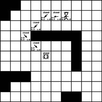
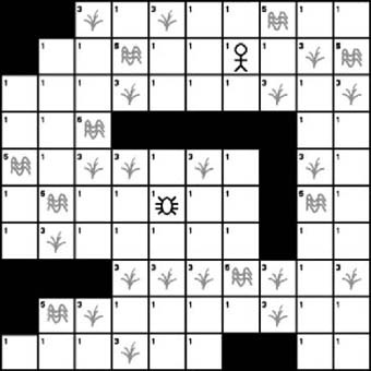
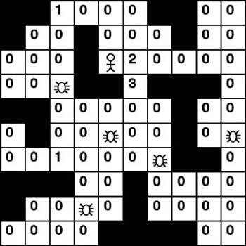
Figure 7-3 shows the tiled search area that we will use. The starting point will be the spider near the center. The desired destination will be the human character. The solid black squares represent wall obstacles, while the white squares represent areas the spider can walk on.

Figure 7-3. Creating a tiled search area

Like any pathfinding algorithm, A∗ will find a path between a starting node and an ending node. It accomplishes this by starting the search at the starting node and then branching out to the surrounding nodes. In the case of this example, it will begin at the starting tile and then spread to the adjacent tiles. This branching out to adjacent tiles continues until we reach the destination node. However, before we start this branching search technique, we need a way to keep track of which tiles need to be searched. This is typically called the open list when using the A∗ algorithm. We begin with just one node in the open list. This is the starting node. We will add more nodes to the open list later. (Note, we’ll use the terms nodes and tiles interchangeably when referring to tiled environments.)

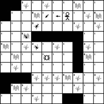
Once we have built the open list, we traverse it and search the tiles adjacent to each tile on the list. The idea is to look at each adjacent tile and determine if it is a valid tile for the path. We basically are checking to see if the adjacent tiles can be walked on by a game character. For example, a road tile would be valid, whereas a wall tile probably would not be valid. We proceed to check each of the eight adjacent tiles and then add each valid tile to the open list. If a tile contains an obstacle, we simply ignore it. It doesn’t get added to the open list. Figure 7-4 shows the tiles adjacent to the initial location that need to be checked.

Figure 7-4. Adjacent tiles to consider

In addition to the open list, the A∗ algorithm also maintains a closed list. The closed list contains the tiles that already were checked and no longer need to be examined. We essentially add a tile to the closed list once all its adjacent tiles have been checked. As Figure 7-5 shows, we have checked each tile adjacent to the starting tile, so the starting tile can be added to the closed list.

Figure 7-5. Moving the starting tile to the closed list

So, as Figure 7-5 shows, the end result is that we now have eight new tiles added to the open list and one tile removed from the open list. The description so far shows the basic iteration through a main A∗ loop; however, we need to track some additional information. We need some way to link the tiles together. The open list maintains a list of adjacent tiles that a character can walk on, but we also need to know how the adjacent tiles link together. We do this by tracking the parent tile of each tile in the open list. A tile’s parent is the single tile that the character steps from to get to its current location. As Figure 7-6 shows, on the first iteration through the loop, each tile will point to the starting tile as its parent.

Figure 7-6. Linking to the parents

Ultimately we will use the parent links to trace a path back to the starting tile once we finally reach the destination. However, we still need to go through a series of additional iterations before we reach the destination.

At this point we begin the process again. We now have to choose a new tile to check from the open list. On the first iteration we had only a single tile on the open list. We now have eight tiles on the open list. The trick now is to determine which member of the open list to check. We determine this by applying a score to each tile.

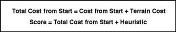
Ultimately, we will use path scoring to determine the best path from the starting tile to the destination tile. To actually score each tile, we basically add together two components. First, we look at the cost to move from the starting tile to any given tile. Next, we look at the cost to move from the given tile to the destination tile. The first component is relatively straightforward. We start our search from the initial location and branch out from there. This makes calculating the cost of moving from the initial location to each tile that we branch out to relatively easy. We simply take the sum of the cost of each tile that leads back to the initial location. Remember, we are saving links to the parents of each tile. Back-stepping to the initial location is a simple matter. However, how do we determine the cost of moving from a given tile to the destination tile? The destination tile is the ultimate goal, which we haven’t reached yet. So, how do we determine the cost of a path that we haven’t determined yet? Well, at this point, all we can do is guess. This is called the heuristic. We essentially make the best guess we can make, given the information we have. Figure 7-7 shows the equation we use for scoring any given tile.

Figure 7-7. Calculating the path score

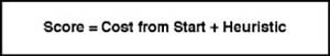
So, we calculate each tile’s score by adding the cost of getting there from the starting location to the heuristic value, which is an estimate of the cost of getting from the given tile to the final destination.

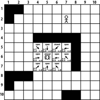
We use this score when determining which tile to check next from the open list. We will first check the tiles with the lowest cost. In this case, a lower cost will equate to a shorter path. Figure 7-8 shows the score, cost, and heuristic applied to each tile we have checked so far.

Figure 7-8. Initial tile path scores

The s value shown in each open tile is the cost of getting there from the starting tile. In this case, each value is 1 because each tile is just one step from the starting tile. The h value is the heuristic. The heuristic is an estimate of the number of steps from the given tile to the destination tile. For example, the tile to the upper right of the starting tile has an h value of 3. That’s because that tile is three steps away from the destination tile. You’ll notice that we don’t take obstacles into consideration when determining the heuristic. We haven’t examined the tiles between the current tile and the destination tile, so we don’t really know yet if they contain obstacles. At this point we simply want to determine the cost, assuming that there are no obstacles. The final value is c, which is the sum of s and h. This is the cost of the tile. It represents the known cost of getting there from the starting point and an estimate of the remaining cost to get to the destination.

Previously, we posed the question of which tile to choose first from the open list on the next iteration through the A∗ algorithm. The answer is the one with the lowest c value. As Figure 7-9 shows, the lowest c value is 4, but we actually have three tiles with that value. Which one should we choose? It doesn’t really matter. Let’s start with the one to the upper right of the starting tile. Assuming that we are using a (row, column) coordinate system where the upper-left coordinate of the search area is position (1, 1), we are now looking at tile (5, 6).

Figure 7-9. Examining tile (5, 6)

The current tile of interest in Figure 7-9 is tile (5, 6), which is positioned to the upper right of the starting location. We now repeat the algorithm we showed you previously where we examine each tile adjacent to the current tile. In the first iteration each tile adjacent to the starting tile was available, meaning they had not yet been examined and they didn’t contain any obstacles. However, that isn’t the case with this iteration. When looking for adjacent tiles, we will only consider tiles that haven’t been examined before and that a game character can walk on. This means we will ignore all tiles on the open list, all tiles on the closed list, or all tiles that contain obstacles. This leaves only two tiles, the one directly to the right of the current tile and the one to the lower right of the current tile. Both tiles are added to the open list. As you can see in Figure 7-9, we create a pointer for each tile added to the open list that points back to its parent tile. We also calculate the s, h, and c values of the new tiles. In this case we calculate the s values by stepping back through the parent link. This tells us how many steps we are from the starting point. Once again, the h value is the heuristic, which is an estimate of the distance from the given tile to the destination. And once again the c value is the sum of s and h. The final step is to add our current tile, the one at position (5, 6), to the closed list. This tile is no longer of any interest to us. We already examined each of its adjacent tiles, so there is no need to examine it again.

We now repeat the process. We have added two new tiles to the open list and moved one to the closed list. We once again search the open list for the tile with the lowest cost. As with the first iteration, the tile with the lowest cost in the open list has a value of 4. However, this time we have only two tiles in the open list with a cost of 4. As before, it really doesn’t matter which we examine first. For this example, we will examine tile (5, 5) next. This is shown in Figure 7-10.

Figure 7-10. Examining tile (5, 5)

As with the previous cases, we examine each tile adjacent to the current tile. However, in this case no available tiles are adjacent to the current tile. They all are either open or closed, or they contain an obstacle. So, as Figure 7-10 shows, we simply have to mark the current tile as closed and then move on.

Now we are down to one single tile in the open list that appears to be superior to the rest. It has a cost of 4, which is the lowest among all the tiles in the open list. It’s located at position (5, 4), which is to the upper left of the starting position. As Figure 7-11 shows, this is the tile we will examine next.

Figure 7-11. Examining tile (5, 4)

As Figure 7-11 shows, we once again examine all the tiles that are adjacent to the current tile. In this case, only three tiles are available: the one to the upper left, the one to the left, and the one to the lower left. The remaining adjacent tiles are either on the open list, are on the closed list, or contain an obstruction. The three new tiles are added to the open list and the current tile is moved to the closed list. We then calculate the scores for the three new tiles and begin the process again.

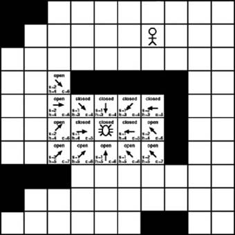
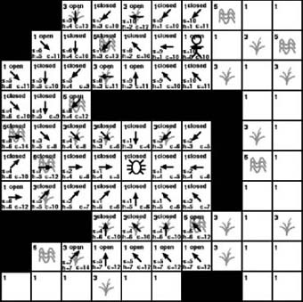
We have added two new tiles to the open list and moved one to the closed list. The previous time we examined the open list we found that the tile with the lowest cost had a value of 4. This time around the tile with the lowest cost on the open list has a value of 5. In fact, three open tiles have a value of 5. Their positions are (5, 7), (6, 6), and (6, 4). Figure 7-12 shows the result of examining each of them. The actual A∗ algorithm would only examine one tile at a time and then only check the additional tiles with the same value if no new tiles with lower values were discovered. However, for purposes of this example, we’ll show the results of examining all of them.

Figure 7-12. Examining all tiles with a cost of 5

As with the previous iterations, each new available tile is added to the open list and each examined tile is moved to the closed list. We also calculate the scores for each new tile. Traversing the open list again tells us that 6 is the lowest score available, so we proceed to examine the tiles with that score. Once again, it doesn’t matter which we check first. As with Figure 7-12, we’ll assume the worst-case scenario in which the best option is selected last. This will show the results of examining all the tiles with a score of 6. This is illustrated in Figure 7-13.

Figure 7-13. Examining all tiles with a cost of 6

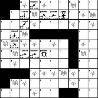
As Figure 7-13 shows, we examined every tile with a cost of 6. As with the previous iterations, new tiles are added to the open list and the examined tiles are moved to the closed list. Once again, the cost values are calculated for the new tiles. As you can see in Figure 7-13, the value of the heuristic is becoming more apparent. The increases in the heuristics of the tiles on the lower portion of the search area are causing noticeable increases to the total cost values. The tiles in the lower part of the search area are still open, so they still might provide the best path to the destination, but for now there are better options to pursue. The lower heuristic values of the open tiles at the top of the search area are making those more desirable. In fact, traversing the open list reveals that the current lowest-cost tile now has a value of 6. In this case, only one tile has a value of 6, tile (3, 4). Figure 7-14 shows the result of examining tile (3, 4).

Figure 7-14. Examining tile (3, 4)

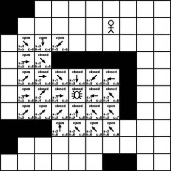
Examining tile (3, 4) results in the addition of three new tiles to the open list. Of course, the current tile at position (3, 4) is then moved to the closed list. As Figure 7-14 shows, most of the tiles on the open list have a cost of 8. Luckily, two of the new tiles added during the previous iteration have a cost of just 6. These are the two tiles we will focus on next. Once again, for purposes of this example, we will assume the worst-case scenario in which it’s necessary to examine both. Figure 7-15 illustrates the results of examining these two tiles.

Figure 7-15. Examining tiles (2, 5) and (3, 5)

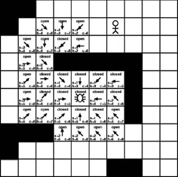
As Figure 7-15 shows, we are finally nearing the destination tile. The previous iteration produced five new tiles for the open list, three of which have a cost of 6, which is the current lowest value. As with the previous iterations, we will now examine all three tiles with a cost value of 6. This is shown in Figure 7-16.

Figure 7-16. Examining tiles (1, 6), (2, 6), and (3, 6)

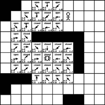
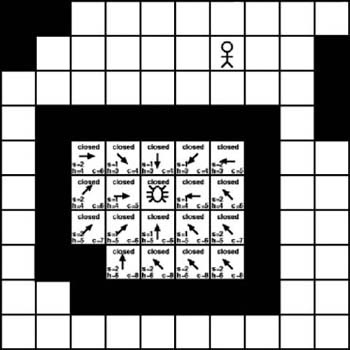
As Figure 7-16 illustrates, we finally reached the destination. However, how does the algorithm determine when we reached it? The answer is simple. The path is found when the destination tile is added to the open list. At that point it’s a simple matter of following the parent links back to the starting point. The only nodes that concern us now are the ones that lead back to the starting node. Figure 7-17 shows the nodes used to build the actual path.

Figure 7-17. The completed path

Once the destination is placed in the open list, we know the path is complete. We then follow the parent links back to the starting tile. In this case, that generates a path made up of the points (2, 7), (2, 6), (2, 5), (3, 4), (4, 3), (5, 4), and (6, 5). If you follow the algorithm we showed here, you’ll always find the shortest possible path. Other paths of equal length might exist, but none will be shorter.

It’s always possible that no valid path exists between any two given points, so how do we know when we have reached a dead end? The simple way to determine if we’ve reached a dead end is to monitor the open list. If we reach the point where no members are in the open list to examine, we’ve reached a dead end. Figure 7-18 shows such a scenario.

Figure 7-18. Dead end

As Figure 7-18 shows, the A∗ algorithm has branched out to every possible adjacent tile. Each one has been examined and moved to the closed list. Eventually, the point was reached where every tile on the open list was examined and no new tiles were available to add. At that point we can conclude that we’ve reached a dead end and that it simply isn’t possible to build a path from the starting point to the desired destination.

As the previous example shows, path scoring already plays a major role in the A∗ algorithm. The standard A∗ algorithm in its most basic form simply determines path cost by the distance traveled. A longer path is considered to be more costly, and hence, less desirable. We often think of a good pathfinding algorithm as one that finds the shortest possible path. However, sometimes other considerations exist. For example, the shortest path isn’t always the fastest path. A game environment can include many types of terrain, all of which can affect the game characters differently. A long walk along a road might be faster than a shorter walk through a swamp. This is where terrain cost comes into play. The previous example shows how we calculate each node’s cost by adding its distance from the initial location to the heuristic value, which is the estimated distance to the destination. It might not have been obvious, but the previous example basically did calculate terrain cost. It just wasn’t very noticeable because all the terrain was the same. Each step the game character took added a value of 1 to the path cost. Basically, every node had the same cost. However, there’s no reason why we can’t assign different cost values to different nodes. It requires just a minor change to the cost equation. We can update the cost equation by factoring in the terrain cost. This is shown in Figure 7-19.

Figure 7-19. Scoring with terrain cost

This results in paths that are longer, but that involve easier terrain. In an actual game this can result in a game character getting from point A to point B in a shorter amount of time, even if the actual path is longer. For example, Figure 7-20 shows several hypothetical types of terrain.

Figure 7-20. Types of terrain

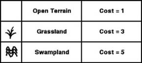
The previous example essentially had only open terrain. The cost of moving from one node to another was always 1. As Figure 7-20 shows, we will now introduce two new types of terrain. The first new terrain type is grassland, which has a cost of 3. The second new type of terrain is swampland, which has a cost of 5. In this case, cost ultimately refers to the amount of time it takes to traverse the node. For example, if it takes a game character one second to walk across a node of open terrain, it will take three seconds to walk across a node of grassland, and five seconds to walk across a node of swampland. The actual physical distances might be equal, but the time it takes to traverse them is different. The A∗ algorithm always searches for the lowest-cost path. If the cost of every node is the same, the result will be the shortest path. However, if we vary the cost of the nodes, the lowest-cost path might no longer be the shortest path. If we equate cost with time, A∗ will find the fastest path rather than the shortest path. Figure 7-21 shows the same tile layout as the previous example, but with the introduction of the terrain elements shown in Figure 7-22.

Figure 7-21. Adding different terrain elements

Figure 7-22. Original path over terrain elements

As you can see in Figure 7-21, the obstacles and game characters are in the same locations as they were in the previous example. The only difference now is the addition of terrain cost. We are no longer looking for the shortest physical path. We now want the fastest path. We are going to assume that grassland takes three times longer to traverse than open terrain does, and that swampland takes five times longer. The question is, how will the added terrain cost affect the path? Figure 7-22 shows the path derived from the previous example.

As Figure 7-22 shows, the shortest path was found. However, you’ll notice that the path is now over several high-cost terrain elements. There is no question that it’s the shortest path, but is there a quicker path? We determine this by using the same A∗ algorithm we stepped through in the first example, but this time we add the terrain cost to the total cost of each node. Figure 7-23 shows the results of following the entire algorithm to its conclusion.

Figure 7-23. Calculating the lowest-cost path

As you can see in Figure 7-23, this is very similar to how we calculated the path in the previous example. We use the same branching technique where we examine the adjacent tiles of the current tile. We then use the same open and closed list to track which tiles need to be examined and which are no longer of interest. The main difference is the s value, which is the cost of moving to any given node from the starting node. We simply used a value of 1 for every node in the previous example. We are now adding the terrain cost to the s value. The resulting lowest-cost path is shown in Figure 7-24.

Figure 7-24. The lowest-cost path

As Figure 7-24 shows, the A∗ algorithm has worked its way around the higher-cost terrain elements. We no longer have the shortest physical path, but we can be assured that no quicker path exists. Other paths might exist that are physically shorter or longer and that would take the same amount of time to traverse, but none would be quicker.

Terrain cost also can be useful when applying the A∗ algorithm to a continuous environment. The previous examples showed how you can apply the A∗ algorithm to a tiled environment where all nodes are equidistant. However, equidistant nodes are not a requirement of the A∗ algorithm. Figure 7-25 shows how nodes could be placed in a continuous environment.

Figure 7-25. Continuous environment node placement

In Figure 7-25, you’ll notice that the distance between the nodes varies. This means that in a continuous environment it will take a longer period of time to traverse the distances between the nodes that are farther apart. This, of course, assumes an equivalent terrain between nodes. However, in this case, the cost of moving between nodes would vary even though the terrain is equivalent. The cost would be equal to the distance between nodes.

We’ve discussed several different types of costs associated with moving between nodes. Although we tend to think of cost as being either time or distance, other possibilities exist, such as money, fuel, or other types of resources.

The previous section showed how different terrain elements can affect how the A∗ algorithm calculates a path. Terrain cost is usually something that the game designer hardcodes into the game world. Basically, we know beforehand where the grasslands, swamplands, hills, and rivers will be located. However, other elements can influence path cost when calculating a path with A∗. For example, nodes that pass through the line of sight of any enemy might present a higher cost. This isn’t a cost that you could build into a game level because the position of the game characters can change. Influence mapping is a way to vary the cost of the A∗ nodes depending on what is happening in the game. This is illustrated in Figure 7-26.

Figure 7-26. Influenced by the enemy firing zone

As Figure 7-26 shows, we have assigned a cost to each node. Unlike the terrain cost we showed you in the previous section, however, this cost is influenced by the position and orientation of the tank shown at position (8, 4). This influence map will change as the tank’s position and orientation change. Like the terrain cost from the previous section, the influence map cost will be added to each node’s s value when calculating possible paths. This will result in the tank’s target possibly taking a longer and slower route when building a path. However, the tiles in the line of fire still are passable, just at a higher cost. If no other path is available, or if the alternate paths have a higher cost, the game character will pass through the line of fire.

You can use influence mapping in other ways to make game characters seem smarter. You can record individual game incidents in an influence map. In this case, we aren’t using the position and orientation of a game character to build an influence map. We are instead using what the character does. For example, if the player repeatedly ambushes and kills computer-controlled characters at a given doorway, that doorway might increase in cost. The computer could then begin to build alternate paths whenever possible. To the player, this can make the computer-controlled characters seem very intelligent. It will appear as though they are learning from their mistakes. This technique is illustrated in Figure 7-27.

Figure 7-27. Influenced by the number of kills

The influence map illustrated in Figure 7-27 records the number of kills the player makes on each node. Each time the player makes a kill, that node increases in cost. For example, there might be a particular doorway where the player has discovered an ambush technique that has led to a series of successful kills. Instead of having the computer-controlled adversaries repeatedly pass through the same doorway, you could create perhaps a longer, but less costly path to offset the player’s tactical advantage.

Steven Woodcock reported in his “2003 Game Developer’s Conference AI Roundtable Moderator’s Report” that AI developers essentially considered pathfinding solved. Other game AI resources all over the Web echo this sentiment. What developers mean is that proven algorithms are available to solve pathfinding problems in a wide variety of game scenarios and most effort these days is focused on optimizing these methods. The workhorse pathfinding method is by far the A∗ algorithm. Current development effort is now focused on developing faster, more efficient A∗ algorithms. Game Programming Gems (Charles River Media) and AI Game Programming Wisdom (Charles River Media) contain several interesting articles on A∗ optimizations.