
Chapter 9. Finite State Machines
A finite state machine is an abstract machine that can exist in one of several different and predefined states. A finite state machine also can define a set of conditions that determine when the state should change. The actual state determines how the state machine behaves.
Finite state machines date back to the earliest days of computer game programming. For example, the ghosts in Pac Man are finite state machines. They can roam freely, chase the player, or evade the player. In each state they behave differently, and their transitions are determined by the player’s actions. For example, if the player eats a power pill, the ghosts’ state might change from chasing to evading. We’ll come back to this example in the next section.
Although finite state machines have been around for a long time, they are still quite common and useful in modern games. The fact that they are relatively easy to understand, implement, and debug contributes to their frequent use in game development. In this chapter, we discuss the fundamentals of finite state machines and show you how to implement them.
Basic State Machine Model
The diagram in Figure 9-1 illustrates how you can model a simple finite state machine.
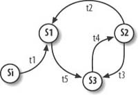
In Figure 9-1, each potential state is illustrated with a circle, and there are four possible states {Si, S1, S2, S3}. Of course, every finite state machine also needs a means to move from one state to another. In this case, the transition functions are illustrated as {t1, t2, t3, t4, t5}. The finite state machine begins with the initial state Si. It remains is this state until the t1 transition function provides a stimulus. Once the stimulus is provided, the state switches to S1. At this point, it’s easy for you to see which stimulus is needed to move from one state to another. In some cases, such as with S1, only the stimulus provided by t5 can change the machine’s state. However, notice that in the case of S3 and S2 two possible stimuli result in a state change.
Now that we’ve shown you a simple state machine model, let’s look at a more practical and slightly more complex example. Figure 9-2 shows a finite state machine that might appear in an actual game.
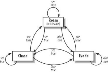
Look closely at Figure 9-2, and you can see that the behavior of the finite state machine models a behavior similar to that of a ghost in Pac Man. Each oval represents a possible state. In this case, there are three possible states: roam, evade, and chase. The arrows show the possible transitions. The transitions show the conditions under which the state can change or remain the same.
In this case, the computer-controlled AI opponent begins in the initial rRoam state. Two conditions can cause a change of state. The first is blue=true. In this case, the AI opponent has turned blue because the player has eaten a power pill. This results in a state change from roam to evade. The other condition that can change the state is see=true, which means the game AI can see the player, resulting in a state change from roam to chase. Now it is no longer necessary to roam freely. The game AI can see and chase the player.
The figure also shows that the finite state machine stays in the evade state as long as it’s blue. Otherwise, the state changes to chase if the player can be seen. If the player can’t be seen, it reverts to the roam state. Likewise, the machine remains in the chase state unless it’s blue, in which case it changes to evade. However, if it’s chasing the player but loses sight of him or her, it once again reverts to the roam state.
Now that we’ve shown how you can model this behavior in a finite state machine diagram, let’s see how you can set up actual program code to implement this behavior. Example 9-1 shows the code.
switch (currentState)
   {
      case kRoam:
          if (imBlue==true) currentState=kEvade;
          else if (canSeePlayer==true) currentState=kChase;
          else if (canSeePlayer==false) currentState=kRoam;
          break;
      case kChase:
          if (imBlue==true) currentState=kEvade;
          else if (canSeePlayer==false) currentState=kRoam;
          else if (canSeePlayer==true) currentState=kChase;
          break;
      case kEvade:
          if (imBlue==true) currentState=kEvade;
          else if (canSeePlayer==true) currentState=kChase;
          else if (canSeePlayer==false) currentState=kRoam;
          break;
   }
The program code in Example 9-1 is not necessarily the most efficient solution to the problem, but it does show how you can use actual program code to model the behavior shown in Figure 9-2. In this case, the switch statement checks for three possible states: kRoam, kChase, and kEvade. Each case in the switch statement then checks for the possible conditions under which the state either changes or remains the same. Notice that in each case the imBlue condition is considered to have precedence. If imBlue is true, the state automatically switches to kEvade regardless of any other conditions. The finite state machine then remains in the kEvade state as long as imBlue is true.
Finite State Machine Design
Now we will discuss some of the methods you can use to implement a finite state machine in a game. Finite state machines actually lend themselves very well to game AI development. They present a simple and logical way to control game AI behavior. In fact, they probably have been implemented in many games without the developer realizing that a finite state machine model was being used.
We’ll start by dividing the task into two components. First, we will discuss the types of structures we will use to store the data associated with the game AI entity. Then we will discuss how to set up the functions we will use to transition between the machine states.
Finite State Machine Structures and Classes
Games that are developed using a high-level language, such as C or C++, typically store all the data related to each game AI entity in a single structure or class. Such a structure can contain values such as position, health, strength, special abilities, and inventory, among many others. Of course, besides all these elements, the structure also stores the current AI state, and it’s the state that ultimately determines the AI’s behavior. Example 9-2 shows how a typical game might store a game AI entity’s data in a single class structure.
class AIEntity
   {
      public:
         int type;
         int state;
         int row;
         int column;
         int health;
         int strength;
         int intelligence;
         int magic;
   };
In Example 9-2, the first element in the class refers to the entity type. This can be anything, such as a troll, a human, or an interstellar battle cruiser. The next element in the class is the one that concerns us most in this chapter. This is where the AI state is stored. The remaining variables in the structure show typical values that generally are associated with a game AI entity.
The state itself typically is assigned using a global constant. Adding a new state is as simple as adding a new global constant. Example 9-3 shows how you can define such constants.
Now that we’ve seen how the AI state and vital statistics are grouped in a single class structure, let’s look at how we can add transition functions to the structure.
Finite State Machine Behavior and Transition Functions
The next step in implementing a finite state machine is to provide functions that determine how the AI entity should behave and when the state should be changed. Example 9-4 shows how you can add behavior and transition functions to an AI class structure.
class	  AIEntity
   {
      public:
         int type;
         int state;
         int row;
         int column;
         int health;
         int strength;
         int intelligence;
         int magic;
         int armed;
         Boolean playerInRange();
         int checkHealth();
   };
You can see that we added two functions to the AIEntity class. Of course, in a real game you probably would use many functions to control the AI behavior and alter the AI state. In this case, however, two transition functions suffice to demonstrate how you can alter an AI entity’s state. Example 9-5 shows how you can use the two transition functions to change the machine state.
if ((checkHealth()<kPoorHealth) && (playerInRange()==false))
   state=kHide;
else if (checkHealth()<kPoorHealth)
   state=kEvade;
else if (playerInRange())
   state=kAttack;
else
   state=kRoam;
The first if statement in Example 9-5 checks to see if the AI entity’s health is low and if the player is not nearby. If these conditions are true, the creature represented by this class structure goes into a hiding state. Presumably, it remains in this state until its health increases. The second if simply checks for poor health. The fact that we’ve reached this if statement means the player is nearby. If that wasn’t the case, the first if statement would have been evaluated as true. Because the player is nearby, hiding might not be practical, as the player might be able to see the AI entity. In this case, it’s more appropriate to attempt to evade the player. The third if statement checks to see if the player is in range. Once again, we know the AI is in good health; otherwise, one of the first two if statements would have been evaluated as true. Because the player is nearby and the AI entity is in good health, the state is changed to attack. The final state option is selected if none of the other options applies. In this case, we go into a default roam state. The creature in this example remains in the roam state until the conditions specified by the transition function indicate that the state should change.
The previous sections showed the basics of setting up a class structure and transition functions for a simple finite state machine. In the next section we go on to implement these concepts into a full-featured finite state machine example.
Ant Example
The objective in this example of our finite state machine is to create a finite state machine simulation consisting of two teams of AI ants. The purpose of the simulation is for the ants to collect food and return it to their home position. The ants will have to follow certain obstacles and rules in the simulation. First, the ants will move randomly in their environment in an attempt to locate a piece of food. Once an ant finds a piece of food, it will return to its home position. When it arrives home, it will drop its food and then start a new search for water rather than food. The thirsty ants will roam randomly in search of water. Once an ant finds water, it will resume its search for more food.
Returning food to the home position also will result in a new ant emerging from the home position. The ant population will continue to grow so long as more food is returned to the home position. Of course, the ants will encounter obstacles along the way. In addition to the randomly placed food will be randomly placed poison. Naturally, the poison has a fatal effect on the ants.
Figure 9-3 presents a finite state diagram that illustrates the behavior of each ant in the simulation.
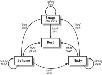
As Figure 9-3 shows, each ant begins in the initial forage state. From that point, the state can change in only two ways. The state can change to go home with the found food transition function, or it can encounter the found poison transition, which kills the ant. Once food is found, the state changes to go home. Once again, there are only two ways out of this state. One is to meet the objective and find the home position. This is illustrated by the found home transition arrow. The other possible transition is to find poison. Once the home position is found, the state changes to thirsty. Like the previous states, there are two ways to change states. One is to meet the goal by finding water, and the other is to find poison. If the goal is met, the ant returns to the initial forage state.
As you can see, the ants will be in one of several different states as they attempt to perform their tasks. Each state represents a different desired behavior. So, we will now use the previously described rules for our simulation to define the possible states for the AI ants. This is demonstrated in Example 9-6.
The first rule for the simulation is that the ants forage randomly for food. This is defined by the kForage state. Any ant in the kForage state moves randomly about its environment in search of food. Once an ant finds a piece of food, it changes to the kGoHome state. In this state, the ant returns to its home position. It no longer forages when in the kGoHome state. It ignores any food it finds while returning home. If the ant successfully returns to its home position without encountering any poison, it changes to the kThirsty state. This state is similar to the forage state, but instead of searching for food the ant searches for water. Once it finds water, the ant changes from the kThirsty state back to the kForage state. At that point the behavior repeats.
Finite State Machine Classes and Structures
Now that we have described and illustrated the basic goal of the finite state machine in our ant simulation, let’s move on to the data structure that we will use. As shown in Example 9-7, we’ll use a C++ class to store all the data related to each finite state machine ant.
#define   kMaxEntities        200
class	    ai_Entity
{
   public:
   int                type;
   int                state;
   int                row;
   int                col;

   ai_Entity();
   ~ai_Entity();

};
ai_Entity     entityList[kMaxEntities];
As Example 9-7 shows, we start with a C++ class containing four variables. The first variable is type, which is the type of AI entity the structure represents.
If you remember from the previous description, the ant simulation consists of two teams of ants. We will differentiate between them by using the constants in Example 9-8.
The second variable in ai_Entity is state. This variable stores the current state of the ant. This can be any of the values defined in Example 9-6; namely, kForage, kGoHome, kThirsty, and kDead.
The final two variables are row and col. The ant simulation takes place in a tiled environment. The row and col variables contain the positions of the ants within the tiled world.
As Example 9-7 goes on to show, we create an array to store each ant’s data. Each element in the array represents a different ant. The maximum number of ants in the simulation is limited by the constant, which also is defined in Example 9-7.
Defining the Simulation World
As we stated previously, the simulation takes place in a tiled environment. The world is represented by a two-dimensional array of integers. Example 9-9 shows the constant and array declarations.
Each element in the terrain array stores the value of a tile in the environment. The size of the world is defined by the kMaxRows and kMaxCols constants. A real tile-based game most likely would contain a large number of possible values for each tile. In this simulation, however, we are using only six possible values. Example 9-10 shows the constants.
   #define   kGround          1
   #define   kWater           2
   #define   kBlackHome       3
   #define   kRedHome         4
   #define   kPoison          5
   #define   kFood            6
The default value in the tile environment is kGround. You can think of this as nothing more than an empty location. The next constant, kWater, is the element the ants search for when in the kThirsty state. The next two constants are kBlackhome and kRedHome. These are the home locations the ants seek out when in the kGoHome state. Stepping on a tile containing the kPoison element kills the ants, changing their states to kDead. The final constant is kFood. When an ant in the kForage state steps on a terrain element containing the kFood element, it changes states from kForage to kGoHome.
Once the variables and constants are declared, we can proceed to initialize the world using the code shown in Example 9-11.
   #define   kRedHomeRow         5
   #define   kRedHomeCol         5

   #define   kBlackHomeRow       5
   #define   kBlackHomeCol      36
   for (i=0;i<kMaxRows;i++)
      for (j=0;j<kMaxCols;j++)
         {
            terrain[i][j]=kGround;
         }
   terrain[kRedHomeRow][kRedHomeCol]=kRedHome;
   terrain[kBlackHomeRow][kBlackHomeCol]=kBlackHome;

   for (i=0;i<kMaxWater;i++)
      terrain[Rnd(2,kMaxRows)-3][Rnd(1,kMaxCols)-1]=kWater;
   for (i=0;i<kMaxPoison;i++)
      terrain[Rnd(2,kMaxRows)-3][Rnd(1,kMaxCols)-1]=kPoison;
   for (i=0;i<kMaxFood;i++)
      terrain[Rnd(2,kMaxRows)-3][Rnd(1,kMaxCols)-1]=kFood;
Example 9-11 starts by initializing the entire two-dimensional world array to the value in kGround. Remember, this is the default value. We then initialize the two home locations. The actual positions are defined in the constants kRedHomeRow, kRedHomeCol, kBlackHomeRow, and kBlackHomeCol. These are the positions the ants move toward when in the kGoHome state. Each ant moves to its respective color.
The final section of Example 9-11 shows three for loops that randomly place the kWater, kPoison, and kFood tiles. The number of each type of tile is defined by its respective constant. Of course, altering these values changes the behavior of the simulation.
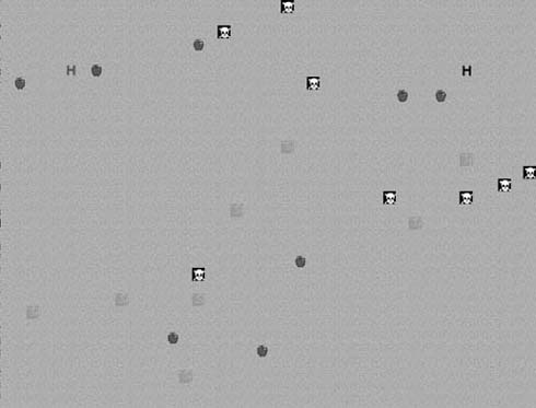
Figure 9-4 shows the result of initializing the tiled world. We haven’t populated the world yet with any finite state machine ants, but we do have the randomly placed food, water, and poison.
Now that we’ve initialized the variables associated with the tile, the next step is to begin populating the world with AI ants.
Populating the World
The first thing we need is some means of creating a new AI entity. To accomplish this, we are going to add a new function to the ai_Entity class. Example 9-12 shows the addition to the ai_Entity class.
class	     ai_Entity
{
   public:
   int                type;
   int                state;
   int                row;
   int                col;

   ai_Entity();
   ~ai_Entity();

   void  New (int theType, int theState, int theRow, int theCol);
};
The New function is called whenever it is necessary to add a new ant to the world. At the beginning of the simulation we add only two of each color ant to the world. However, we call this function again whenever an ant successfully returns food to the home position. Example 9-13 shows how the actual function is defined.
void ai_Entity::New(int  theType, int theState, int theRow, int theCol)
{
   int   i;

   type=theType;
   row=theRow;
   col=theCol;
   state=theState;
}
The New function is rather simple. It initializes the four values in ai_Entity. These include the entity type, state, row, and column. Now let’s look at Example 9-14 to see how the New function adds ants to the finite state machine simulation.
   entityList[0].New(kRedAnt,kForage,5,5);
   entityList[1].New(kRedAnt,kForage,8,5);

   entityList[2].New(kBlackAnt,kForage,5,36);
   entityList[3].New(kBlackAnt,kForage,8,36);
As Example 9-14 shows, the simulation begins by adding four ants to the world. The first parameter passed to the New function specifies the entity type. In this simulation, we start with two red ants and two black ants. The second parameter is the initial state of the finite state machine ants. The final two parameters are the row and column positions of the starting point of each ant.
As Figure 9-5 shows, we added four ants to the simulation using the New function.
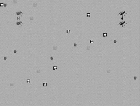
Each ant shown in Figure 9-5 begins with its initial state set to kForage. From their initial starting positions they will begin randomly moving about the tiled environment in search of food. In this case, the food is shown as apples. However, if they step on poison, shown as a skull and crossbones, they switch to the kDead state. The squares containing the water pattern are the elements they search for when they are in the kThirsty state.
Updating the World
In the previous section we successfully populated the world with four finite state machine ants. Now we will show you how to run the simulation. This is a critical part of the finite state machine implementation. If you recall, the basic premise of the finite state machine is to link individual and unique states to different types of behavior. This is the part of the code where we actually make each ant behave a certain way depending on its state. This part of the code lends itself to the use of a switch statement, which checks for each possible state. In a real game, this switch statement typically would be called once each time through the main loop. Example 9-15 shows how to use the switch statement.
   for (i=0;i<kMaxEntities;i++)
      {
         switch (entityList[i].state)
            {
               case kForage:
                  entityList[i].Forage();
                  break;
               case kGoHome:
                  entityList[i].GoHome();
                  break;
               case kThirsty:
                  entityList[i].Thirsty();
                  break;
               case kDead:
                  entityList[i].Dead();
                  break;
            }
      }
As Example 9-15 shows, we create a loop that iterates through each element in the entityList array. Each entityList element contains a different finite state machine ant. We use a switch statement to check the state of each ant in entityList. Notice that we have a case statement for each possible state. We then link each state to the desired behavior by calling the appropriate function for each behavior. As you can see in Example 9-16, we need to add four new functions to the ai_Entity class.
class	   ai_Entity
{
   public:
   int                type;
   int                state;
   int                row;
   int                col;

   ai_Entity();
   ~ai_Entity();

   void  New (int theType, int theState, int theRow, int theCol);
   void Forage(void);
   void GoHome(void);
   void Thirsty(void);
   void Dead(void);
};
Example 9-16 shows the updated ai_Entity class with the four new behavior functions. Each function is associated with one of the state behaviors.
Forage
The first new function, Forage, is associated with the kForage state. If you recall, in this state the ants randomly move about the world in search of food. Once in the forage state, the ants can switch to a different state in only two ways. The first way is to meet the objective by randomly finding a piece of food. In this case, the state switches to kGoHome. The other way for the ants to switch states is by stepping on poison. In this case, the state switches to kDead. This behavior is implemented in the Forage function, as shown in Example 9-17.
void ai_Entity::Forage(void)
{
   int rowMove;
   int colMove;
   int newRow;
   int newCol;
   int foodRow;
   int foodCol;
   int poisonRow;
   int poisonCol;
   rowMove=Rnd(0,2)-1;
   colMove=Rnd(0,2)-1;
   newRow=row+rowMove;
   newCol=col+colMove;
   if (newRow<1) return;
   if (newCol<1) return;
   if (newRow>=kMaxRows-1) return;
   if (newCol>=kMaxCols-1) return;
   if ((terrain[newRow][newCol]==kGround) ||
       (terrain[newRow][newCol]==kWater))
      {
         row=newRow;
         col=newCol;
      }
   if (terrain[newRow][newCol]==kFood)
      {
         row=newRow;
         col=newCol;
         terrain[row][col]=kGround;
         state=kGoHome;
         do {
            foodRow=Rnd(2,kMaxRows)-3;
            foodCol=Rnd(2,kMaxCols)-3;
         } while (terrain[foodRow][foodCol]!=kGround);
         terrain[foodRow][foodCol]=kFood;
      }
   if (terrain[newRow][newCol]==kPoison)
      {
         row=newRow;
         col=newCol;
         terrain[row][col]=kGround;
         state=kDead;
         do {
            poisonRow=Rnd(2,kMaxRows)-3;
            poisonCol=Rnd(2,kMaxCols)-3;
         } while (terrain[poisonRow][poisonCol]!=kGround);
         terrain[poisonRow][poisonCol]=kPoison;
      }
}
contain the distances to move in both the row and column directions. The next two variables are newRow and newCol. These two variables contain the new row and column positions of the ant. The final four variables, foodRow, foodCol, poisonRow, and poisonCol, are the new positions used to replace any food or poison that might get consumed.
We then proceed to calculate the new position. We begin by assigning a random number between −1 and +1 to the rowMove and colMove variables. This ensures that the ant can move in any of the eight possible directions in the tiled environment. It’s also possible that both values will be 0, in which case the ant will remain in its current position.
Once we have assigned rowMove and colMove, we proceed to add their values to the current row and column positions and store the result in newRow and newCol. This will be the new ant position, assuming, of course, it’s a legal position in the tiled environment. In fact, the next block of if statements checks to see if the new position is within the legal bounds of the tiled environment. If it’s not a legal position, we exit the function.
Now that we know the position is legal, we go on to determine what the ant will be standing on in its new position. The first if statement simply checks for kGround or kWater at the new position. Neither of these two elements will cause a change in state, so we simply update the ant row and col with the values in newRow and newCol. The ant is shown in its new position after the next screen update.
The next section shows a critical part of the finite state machine design. This if statement checks to see if the new position contains food. This section is critical because it contains a possible state transition. If the new position does contain food, we update the ant’s position, erase the food, and change the state of the ant. In this case, we are changing from kForage to kGoHome. The final do-while loop in this if statement replaces the consumed food with another randomly placed piece of food. If we don’t continuously replace the consumed food, the ant population won’t be able to grow.
The final part of the Forage function shows another possible state transition. The last if statement checks to see if the new position contains poison. If it does contain poison, the ant’s position is updated, the poison is deleted, and the ant’s state is changed from kForage to kDead. We then use the do-while loop to replenish the consumed poison.
GoHome
We are now going to move on to the second new behavior function that we added to the ai_Entity class in Example 9-16. This one is called GoHome and it’s associated with the kGoHome state. As we stated previously, the ants switch to the kGoHome state once they randomly find a piece of food. They remain in this state until they either successfully return to their home position or step on poison. Example 9-18 shows the GoHome function.
void ai_Entity::GoHome(void)
{
   int   rowMove;
   int   colMove;
   int   newRow;
   int   newCol;
   int   homeRow;
   int   homeCol;
   int   index;
   int   poisonRow;
   int   poisonCol;
   if (type==kRedAnt)
      {
         homeRow=kRedHomeRow;
         homeCol=kRedHomeCol;
      }
   else
      {
         homeRow=kBlackHomeRow;
         homeCol=kBlackHomeCol;
      }
   if (row<homeRow)
      rowMove=1;
   else if (row>homeRow)
      rowMove=-1;
   else
      rowMove=0;
   if (col<homeCol)
      colMove=1;
   else if (col>homeCol)
      colMove=-1;
   else
      colMove=0;
   newRow=row+rowMove;
   newCol=col+colMove;
   if (newRow<1) return;
   if (newCol<1) return;
   if (newRow>=kMaxRows-1) return;
   if (newCol>=kMaxCols-1) return;
   if (terrain[newRow][newCol]!=kPoison)
      {
         row=newRow;
         col=newCol;
      }
   else
      {
         row=newRow;
         col=newCol;
         terrain[row][col]=kGround;
         state=kDead;
         do {
            poisonRow=Rnd(2,kMaxRows)-3;
            poisonCol=Rnd(2,kMaxCols)-3;
         } while (terrain[poisonRow][poisonCol]!=kGround);
         terrain[poisonRow][poisonCol]=kPoison;
      }
   if ((newRow==homeRow) && (newCol==homeCol))
      {
         row=newRow;
         col=newCol;
         state=kThirsty;
         for (index=0; index <kMaxEntities; index ++)
            if (entityList[index].type==0)
               {
                  entityList[index].New(type,
                                        kForage,
                                        homeRow,
                                        homeCol);
                  break;
               }
      }
}
The variable declarations in the GoHome function are very similar to those in the Forage function. In this function, however, we added two new variables, homeRow and homeCol. We will use these two variables to determine if the ant has successfully reached its home position. The variable index is used when adding a new ant to the world. The remaining two variables, poisonRow and poisonCol, are used to replace any poison that might be consumed.
We start by determining where the home position is located. If you recall, there are two types of ants, red ants and black ants. Each color has a different home position. The positions of each home are set in the globally defined constants kRedHomeRow, kRedHomeCol, kBlackHomeRow, and kBlackHomeCol. We check the entity type to determine if it’s a red ant or a black ant. We then use the global home position constants to set the local homeRow and homeCol variables. Now that we know where the home is located, we can move the ant toward that position.
As you might recall, this is a variation of the simple chasing algorithm from Chapter 2. If the ant’s current row is less than the home row, the row offset, rowMove, is set to 1. If the ant’s row is greater than the home row, rowMove is set to −1. If they are equal, there is no need to change the ant’s row, so rowMove is set to 0. The column positions are handled the same way. If the ant’s column is less than the home column, colMove is set to 1. If it’s greater, it’s set to −1. If col is equal to homeCol, colMove is set to 0.
Once we have the row and column offsets, we can proceed to calculate the new row and column positions. We determine the new row position by adding rowMove to the current row position. We determine the new column position by adding colMove to the current column position.
Once we assign the values to newRow and newCol, we check to see if the new position is within the bounds of the tiled environment. It’s good practice to always do this, but in this case, it’s really not necessary. This function always moves the ants toward their home position, which always should be within the confines of the tiled world. So, the ants always will be confined to the limits of the world unless the global home position constants are changed to something outside the limits of the world.
The first part of the if statement checks to see if the ant did not step on poison. If the new position does not contain poison, the ant’s position is updated. If the else portion of the if statement gets executed, we know the ant has, in fact, stepped on poison. In this case, a state change is required—the ant’s position is updated, the poison is deleted, and the ant’s state is changed from kGoHome to kDead. We then use the do-while loop to replace the consumed poison.
The final if statement in the GoHome function checks to see if the goal was achieved. It uses the values we assigned to homeRow and homeCol to determine if the new position is equal to the home position. If so, the ant’s position is updated and the state is switched from kGoHome to kThirsty. This will make the ant assume a new behavior the next time the UpdateWorld function is executed. The final part of the if statement is used to generate a new ant. If you recall, whenever food is successfully returned to the home position, a new ant is spawned. We use a for loop to traverse the entityList and check for the first unused element in the array. If an unused array element is found, we create a new ant at the home position and initialize it to the kForage state.
Thirsty
The next behavior function we added to the ai_Entity class in Example 9-16 is associated with the kThirsty state. As you recall, the ants are switched to the kThirsty state after successfully returning food to their home positions. In this state, the ants randomly move about the world in search of water. Unlike the kForage state, however, the ants don’t return to the home position after meeting their goal. Instead, when the ants find water, the state switches from kThirsty back to kForage. As with the previous states, stepping on poison automatically changes the state to kDead.
The third new behavior function we added to the ai_Entity class is called Thirsty, and as the name implies, it’s executed when the ants are in the kThirsty state. As we stated previously, the ants switch to the kThirsty state after successfully returning food to their home positions. They remain in the kThirsty state until they find water or until they step on poison. If they find water, they revert to their initial kForage state. If they step on poison, they switch to the kDead state. Example 9-19 shows the Thirsty function.
void ai_Entity::Thirsty(void)
{
   int   rowMove;
   int   colMove;
   int   newRow;
   int   newCol;
   int   foodRow;
   int   foodCol;
   int   poisonRow;
   int   poisonCol;
   rowMove=Rnd(0,2)-1;
   colMove=Rnd(0,2)-1;
   newRow=row+rowMove;
   newCol=col+colMove;
   if (newRow<1) return;
   if (newCol<1) return;
   if (newRow>=kMaxRows-1) return;
   if (newCol>=kMaxCols-1) return;
   if ((terrain[newRow][newCol]==kGround) ||
       (terrain[newRow][newCol]==kFood))
      {
         row=newRow;
         col=newCol;
      }
   if (terrain[newRow][newCol]==kWater)
      {
         row=newRow;
         col=newCol;
         terrain[row][col]=kGround;
         state=kForage;
         do {
            foodRow=Rnd(2,kMaxRows)-3;
            foodCol=Rnd(2,kMaxCols)-3;
         } while (terrain[foodRow][foodCol]!=kGround);
         terrain[foodRow][foodCol]=kWater;
      }
   if (terrain[newRow][newCol]==kPoison)
      {
         row=newRow;
         col=newCol;
         terrain[row][col]=kGround;
         state=kDead;
         do {
            poisonRow=Rnd(2,kMaxRows)-3;
            poisonCol=Rnd(2,kMaxCols)-3;
         } while (terrain[poisonRow][poisonCol]!=kGround);
         terrain[poisonRow][poisonCol]=kPoison;
      }
}
As you can see in Example 9-19, the Thirsty function begins much like the Forage function. We declare two position offset variables, rowMove and colMove, and two variables for the new ant position, newRow and newCol. The remaining variables, foodRow, foodCol, poisonRow, and poisonCol, are used when replacing consumed food and poison.
We then calculate a random offset for both the row and column positions. Both the rowMove and colMove variables contain a random value between −1 and +1. We add these random values to the current positions to get the new position. The new position is stored in newRow and newCol. The block of if statements determines if the new position is within the bounds of the world. If it’s not, we immediately exit the function.
This if statement checks to see if the new position is an empty tile or a tile containing food. In other words, it doesn’t contain either of the two elements that would cause a change in state.
The next if statement checks to see if the new position contains water. If it does contain water, the ant’s position is updated, the water is deleted, and the ant’s state is changed back to the initial kForage state. The do-while loop then randomly places more water.
As in the previous behavior function, the final if statement in the Thirsty function checks to see if the ant stepped on poison. If so, the ant’s position is updated, the poison is deleted, and the ant’s state is changed to kDead. Once again, the do-while loop is used to replace the consumed poison.
The Results
This completes all four functions associated with the kForage, kThirsty, kGoHome, and kDead states. You can observe the different behaviors and how the finite state machine ants transition from one state to another by running the simulation.
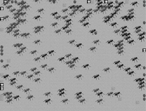
As you can see in Figure 9-6, even though we started with only four ants in the simulation, it doesn’t take long for them to overrun the world. In fact, it’s interesting to watch how quickly they begin multiplying with the given amount of food, water, and poison.
It’s also interesting to watch how you can affect the population growth, or decline, by simply altering the values shown in Example 9-20.
   #define  kMaxWater      15
   #define  kMaxPoison      8
   #define  kMaxFood       20
As Example 9-20 shows, altering the simulation is as simple as modifying a few global constants. For example, decreasing the poison level too much causes a rapid population explosion, while lowering the food supply slows the population growth, but doesn’t necessarily cause it to decrease. By adjusting these values, along with the possibility of adding more states and, therefore, more types of behavior, you can make the simulation even more complex and interesting to watch.
Further Information
Finite state machines are ubiquitous in games. It’s no surprise that virtually every game development book covers them to some degree. Further, the Internet is full of resources covering finite state machines. Here are just a few Internet resources that discuss finite state machines:
If you perform an Internet search using the keywords “finite state machine,” you’re sure to find a few hundred more resources. Also, try performing a search using the keywords “fuzzy state machine.” Fuzzy state machines are a popular variant of finite state machines that incorporate probability in state transitions. We cover probability in Chapter 12.