
Chapter 10. Fuzzy Logic
In 1965 Lotfi Zadeh, a professor at the University of California Berkeley, wrote his original paper laying out fuzzy set theory. We find no better way of explaining what fuzzy logic is than by quoting the father of fuzzy logic himself. In a 1994 interview of Zadeh conducted by Jack Woehr of Dr. Dobbs Journal, Woehr paraphrases Zadeh when he says “fuzzy logic is a means of presenting problems to computers in a way akin to the way humans solve them.” Zadeh later goes on to say that “the essence of fuzzy logic is that everything is a matter of degree.” We’ll now elaborate on these two fundamental principles of fuzzy logic.
What does the statement “problems are presented to computers in a way similar to how humans solve them” really mean? The idea here is that humans very often analyze situations, or solve problems, in a rather imprecise manner. We might not have all the facts, the facts might be uncertain, or perhaps we can only generalize the facts without the benefit of precise data or measurements.
For example, say you’re playing a friendly game of basketball with your buddies. When sizing up an opponent on the court to decide whether you or someone else should guard him, you might base your decision on the opponent’s height and dexterity. You might decide the opponent is tall and quick, and therefore, you’d be better off guarding someone else. Or perhaps you’d say he is very tall but somewhat slow, so you might do fine against him. You normally wouldn’t say to yourself something such as, “He’s 6 feet 5.5 inches tall and can run the length of the court in 5.7 seconds.”
Fuzzy logic enables you to pose and solve problems using linguistic terms similar to what you might use; in theory you could have the computer, using fuzzy logic, tell you whether to guard a particular opponent given that he is very tall and slow, and so on. Although this is not necessarily a practical application of fuzzy logic, it does illustrate a key point—fuzzy logic enables you to think as you normally do while using very precise tools such as computers.
The second principle, that everything is a matter of degree, can be illustrated using the same basketball opponent example. When you say the opponent is tall versus average or very tall, you don’t necessarily have fixed boundaries in mind for such distinctions or categories. You can pretty much judge that the guy is tall or very tall without having to say to yourself that if he is more than 7 feet, he’s very tall, whereas if he is less than 7 feet, he’s tall. What about if he is 6 feet 11.5 inches tall? Certainly you’d still consider that to be very tall, though not to the same degree as if he were 7 feet 4 inches. The border defining your view of tall versus very tall is rather gray and has some overlap.
Traditional Boolean logic forces us to define a point above which we’d consider the guy very tall and below which we’d consider the guy just tall. We’d be forced to say he is either very tall or not very tall. You can circumvent this true or false/on or off characteristic of traditional Boolean logic using fuzzy logic. Fuzzy logic allows gray areas, or degrees, of being very tall, for example.
In fact, you can think of everything in terms of fuzzy logic as being true, but to varying degrees. If we say that something is true to degree 1 in fuzzy logic, it is absolutely true. A truth to degree 0 is an absolute false. So, in fuzzy logic we can have something that is either absolutely true, or absolutely false, or anything in between—something with a degree between 0 and 1. We’ll look at the mechanisms that enable us to quantify degrees of truth a little later.
Another aspect of the ability to have varying degrees of truth in fuzzy logic is that in control applications, for example, responses to fuzzy input are smooth. Using traditional Boolean logic forces us to switch response states to some given input in an abrupt manner. To alleviate very abrupt state transitions, we’d have to discretize the input into a larger number of sufficiently small ranges. We can avoid these problems using fuzzy logic because the response will vary smoothly given the degree of truth, or strength, of the input condition.
Let’s consider an example. A standard home central air conditioner is equipped with a thermostat, which the homeowner sets to a specific temperature. Given the thermostat’s design, it will turn on when the temperature rises higher than the thermostat setting and cut off when the temperature reaches or falls lower than the thermostat setting. Where we’re from in Southern Louisiana, our air conditioner units constantly are switching on and off as the temperature rises and falls due to the warming of the summer sun and subsequent cooling by the air conditioner. Such switching is hard on the air conditioner and often results in significant wear and tear on the unit.
One can envision in this scenario a fuzzy thermostat that modulates the cooling fan so as to keep the temperature about ideal. As the temperature rises the fan speeds up, and as the temperature drops the fan slows down, all the while maintaining some equilibrium temperature right around our prescribed ideal. This would be done without the unit having to switch on and off constantly. Indeed, such systems do exist, and they represent one of the early applications of fuzzy control. Other applications that have benefited from fuzzy control include train and subway control and robot control, to name a few.
Fuzzy logic applications are not limited to control systems. You can use fuzzy logic for decision-making applications as well. One typical example includes stock portfolio analysis or management, whereby one can use fuzzy logic to make buy or sell decisions. Pretty much any problem that involves decision making based on subjective, imprecise, or vague information is a candidate for fuzzy logic.
Traditional logic practitioners argue that you also can solve these problems using traditional rules-based approaches and logic. That might be true; however, fuzzy logic affords us the use of intuitive linguistic terms such as near, far, very far, and so on, when setting up the problem, developing rules, and assessing output. This usually makes the system more readable and easier to understand and maintain. Further, Timothy Masters, in his book Practical Neural Network Recipes in C++, (Morgan Kauffman) reports that fuzzy-rules systems generally require 50% to 80% fewer rules than traditional rules systems to accomplish identical tasks. These benefits make fuzzy logic well worth taking a look at for game AI that is typically replete with if-then style rules and Boolean logic. With this motivation, let’s consider a few illustrative examples of how we can use fuzzy logic in games.
How Can You Use Fuzzy Logic in Games?
You can use fuzzy logic in games in a variety of ways. For example, you can use fuzzy logic to control bots or other nonplayer character units. You also can use it for assessing threats posed by players. Further, you can use fuzzy logic to classify both player and nonplayer characters. These are only a few specific examples, but they illustrate how you can use fuzzy logic in distinctly different scenarios. Let’s consider each example in a little more detail.
Control
Fuzzy logic is used in a wide variety of real-world control applications such as controlling trains, air conditioning and heating systems, and robots, among other applications. Video games also offer many opportunities for fuzzy control. You can use fuzzy control to navigate game units—land vehicles, aircraft, foot units, and so on—smoothly through waypoints and around obstacles. You also can accomplish as well as improve upon basic chasing and evading using fuzzy control.
Let’s say you have a unit that is traveling along some given heading, but it needs to travel toward some specific target that might be static or on the move. This target could be a waypoint, an enemy unit, some treasure, a home base, or anything else you can imagine in your game. We can solve this problem using deterministic methods similar to those we’ve already discussed in this book; however, recall that in some cases we had to manually modulate steering forces to achieve smooth turns. If we didn’t modulate the steering forces, the units abruptly would change heading and their motion would appear unnatural. Fuzzy logic enables you to achieve smooth motion without manually modulating steering forces. You also can gain other improvements using fuzzy logic. For example, recall the problem with basic chasing whereby the unit always ended up following directly behind the target moving along one coordinate axis only. Earlier we solved this problem using other methods, such as line-of-sight chasing, interception, or potential functions. Fuzzy logic, in this case, would yield results similar to interception. Basically, we’d tell our fuzzy controller that our intended target is to the far left, or to the left, or straight ahead, or to the right, and so on, and let it calculate the proper steering force to apply to facilitate heading toward the target in a smooth manner.
Threat Assessment
Let’s consider another potential application of fuzzy logic in games; one that involves a decision rather than direct motion control.
Say in your battle simulation game the computer team often has to deploy units as defense against a potentially threatening enemy force. We’ll assume that the computer team has acquired specific knowledge of an opposing force. For simplicity, we’ll limit this knowledge to the enemy force’s range from the computer team and the force’s size. Range can be specified in terms of near, close, far, and very far, while size can be specified in terms of tiny, small, medium, large, or massive.
Given this information, we can use a fuzzy system to have the computer assess the threat posed by the enemy force. For example, the threat could be considered as no threat, low threat, medium threat, or high threat, upon determination of which the computer could decide on a suitable number of units to deploy in defense. This fuzzy approach would enable us to do the following:
Model the computer as having less-than-perfect knowledge
Allow the size of the defensive force to vary smoothly and less predictably
Classification
Let’s say you want to rank both player and nonplayer characters in your game in terms of their combat prowess. You can base this rank on factors such as strength, weapon proficiency, number of hit points, and armor class, among many other factors of your choosing. Ultimately, you want to combine these factors so as to yield a ranking such as wimpy, easy, moderate, tough, formidable, etc. For example, a player with high hit points, average armor class, high strength, and low weapons proficiency might get a rank of moderate. Fuzzy logic enables you to determine such a rank. Further, you can use the fuzzy logic system to generate a numerical score representing rank, or rating, which you can input to some other AI process for the game.
Of course, you can accomplish this classification by other means, such as Boolean rules, neural networks, and others. However, a fuzzy system enables you to do it in an intuitive manner with fewer rules and without the need to train the system. You still have to set up the fuzzy rules ahead of time, as in every fuzzy system; however, you have to perform that process only once, and you have the linguistic constructs afforded by fuzzy logic to help you. We’ll come back to this later.
Fuzzy Logic Basics
Now that you have an idea of what fuzzy logic is all about and how you can use it in games, let’s take a close look at how fuzzy logic works and is implemented. If the concept of fuzzy logic is still a little, well, fuzzy to you at this point, don’t worry. The concepts will become much clearer as we go over the details in the next few sections.
Overview
The fuzzy control or inference process comprises three basic steps. Figure 10-1 illustrates these steps.
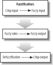
The first part of the process is called the fuzzification process. In this step, a mapping process converts crisp data (real numbers) to fuzzy data. This mapping process involves finding the degree of membership of the crisp input in predefined fuzzy sets. For example, given a person’s weight in pounds, we can find the degree to which the person is underweight, overweight, or at an ideal weight.
Once you have expressed all the inputs to the system in terms of fuzzy set membership, you can combine them using logical, fuzzy rules to determine the degree to which each rule is true. In other words, you can find the strength of each rule or the degree of membership in an output, or action, fuzzy set. For example, given a person’s weight and activity level as input variables, we can define rules that look something such as the following:
If overweight AND NOT active then frequent exercise
If overweight AND active then moderate diet
These rules combine the fuzzy input variables using logical operators to yield a degree of membership, or degree or truth, of the corresponding output action, which in this case is the recommendation to engage in frequent exercise or go on a moderate diet.
Often, having a fuzzy output such as frequent exercise is not enough. We might want to quantify the amount of exercise—for example, three hours per week. This process of taking fuzzy output membership and producing a corresponding crisp numerical output is called defuzzification. Let’s consider each step in more detail.
Fuzzification
Input to a fuzzy system can originate in the form of crisp numbers. These are real numbers quantifying the input variables—for example, a person weighs 185.3 pounds or a person is 6 feet 1 inch tall. In the fuzzification process we want to map these crisp values to degrees of membership in qualitative fuzzy sets. For example, we might map 185.3 pounds to slightly overweight and 6 feet 1 inch to tall. You achieve this type of mapping using membership functions, also called characteristic functions.
Membership Functions
Membership functions map input variables to a degree of membership, in a fuzzy set, between 0 and 1. If the degree of membership in a given set is 1, we can say the input for that set is absolutely true. If the degree is 0, we can say for that set the input is absolutely false. If the degree is somewhere between 0 and 1, it is true to a certain extent—that is, to a degree.
Before looking at fuzzy membership functions, let’s consider the membership function for Boolean logic. Figure 10-2 illustrates such a function.
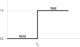
Here we see that input values lower than x 0 are mapped to false, while values higher than x 0 are mapped to true. There is no in-between mapping. Going back to the weight example, if x 0 equals 170 pounds, anyone weighing more than 170 pounds is overweight and anyone weighing less than 170 pounds is not overweight. Even if a person weighs 169.9 pounds, he still is considered not overweight. Fuzzy membership functions enable us to transition gradually from false to true, or from not overweight to overweight in our example.
You can use virtually any function as a membership function, and the shape usually is governed by desired accuracy, the nature of the problem being considered, experience, and ease of implementation, among other factors. With that said, a handful of commonly used membership functions have proven useful for a wide variety of applications. We’ll discuss those common membership functions in this chapter.
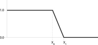
Consider the grade function illustrated in Figure 10-3.
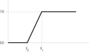
Here you can see the gradual transition from 0 to 1. The range of x-values for which this function applies is called its support. For values less than x 0, the degree of membership is 0 or absolutely false, while for values greater than x 1, the degree is 1 or absolutely true. Between x 0 and x 1, the degree of membership varies linearly.
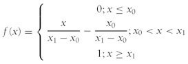
Using the point-slope equation for a straight line, we can write the equation representing the grade membership function as follows:
Going back to the weight example, let’s say this function represents the membership for overweight. Let x 0 equal 175 and x 1 equal 195. If a person weighs 170 pounds, he is overweight to a degree of 0—that is, he is not overweight. If he weighs 185 pounds, he is overweight to a degree of 0.5—he’s somewhat overweight.
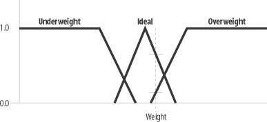
Typically, we’re interested in the degree to which an input variable falls within a number of qualitative sets. For example, we might want to know the degree to which a person is overweight, underweight, or at an ideal weight. In this case, we could set up a collection of sets, as illustrated in Figure 10-4.
The equation for a straight line passing through the points (x0,y0) and (x1 y1) is:
where m is the slope of the line and is equal to:
With this sort of collection, we can calculate a given input value’s membership in each of the three sets—underweight, ideal, and overweight. We might, for a given weight, find that a person is underweight to a degree of 0, ideal to a degree of 0.75, and overweight to a degree of 0.15. We can infer in this case that the person’s weight is substantially ideal—that is, to a degree of 75%.
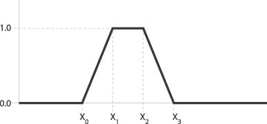
The triangular membership function shown in Figure 10-4 is another common form of membership function. Referring to Figure 10-5, you can write the equation for a triangular membership function as follows:
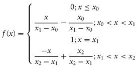
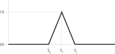
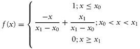
Figure 10-4 also shows a reverse-grade membership function for the underweight set. Referring to Figure 10-6, you can write the equation for the reverse grade as follows:
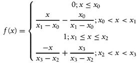
Another common membership function is the trapezoid function, as shown in Figure 10-7.
You can write the trapezoid function as follows:
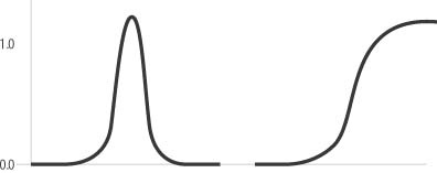
Setting up collections of fuzzy sets for a given input variable, as shown in Figure 10-4, is largely a matter of judgment and trial and error. It’s not uncommon to tune the arrangement of set membership functions to achieve desirable or optimum results. While tuning, you can try different shapes for each fuzzy set, or you can try using more or fewer fuzzy sets. Some fuzzy logic practitioners recommend the use of seven fuzzy sets to fully define the practical working range of any input variable. Figure 10-8 illustrates such an arrangement.
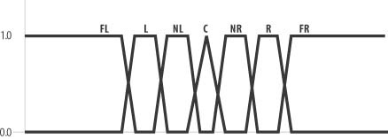
The seven fuzzy sets shown in Figure 10-8 are center, near right, right, far right, near left, left, and far left. These categories can be anything, depending on your problem. For example, to represent the alignment of player and nonplayer characters in your role-playing game, you might have fuzzy sets such as neutral, neutral good, good, chaotic good, neutral evil, evil, and chaotic evil.
Notice that each set in Figures 10-4 and 10-8 overlaps immediately adjacent sets. This is important for smooth transitions. The generally accepted rule of thumb is that each set should overlap its neighbor by about 25%.
The membership functions we discussed so far are the most commonly used; however, other functions sometimes are employed when higher accuracy or nonlinearity is required. For example, some applications use Gaussian curves, while others use S-shaped curves. These are illustrated in Figure 10-9. For most applications and games, the piecewise linear functions discussed here are sufficient.
Example 10-1 shows how the various membership functions we’ve discussed might look in code.
double     FuzzyGrade(double value, double x0, double x1)
{
      double result = 0;
      double x = value;
      if(x <= x0)
            result = 0;
      else if(x >= x1)
            result = 1;
      else
            result = (x/(x1-x0))-(x0/(x1-x0));
      return result;
}
double  FuzzyReverseGrade(double value, double x0, double x1)
{
      double result = 0;
      double x = value;
      if(x <= x0)
            result = 1;
      else if(x >= x1)
            result = 0;
      else
            result = (-x/(x1-x0))+(x1/(x1-x0));
      return result;
}
double     FuzzyTriangle(double value, double x0,
                               double x1, double x2)
{
      double result = 0;
      double x = value;
      if(x <= x0)
             result = 0;
      else if(x == x1)
             result = 1;
      else if((x>x0) && (x<x1))
             result = (x/(x1-x0))-(x0/(x1-x0));
      else
             result = (-x/(x2-x1))+(x2/(x2-x1));
      return result;
}
double     FuzzyTrapezoid(double value, double x0, double x1,
                                double x2, double x3)
{
      double result = 0;
      double x = value;
      if(x <= x0)
             result = 0;
      else if((x>=x1) && (x<=x2))
             result = 1;
      else if((x>x0) && (x<x1))
             result = (x/(x1-x0))-(x0/(x1-x0));
      else
             result = (-x/(x3-x2))+(x3/(x3-x2));
      return result;
}
To determine the membership of a given input value in a particular set, you simply call one of the functions in Example 10-1, passing the value and parameters that define the shape of the function. For example, FuzzyTrapezoid(value, x0, x1, x2, x3) determines the degree of membership of value in the set defined by x0, x1, x2, x3 with a shape, as shown in Figure 10-7.
Hedges
Hedge functions are sometimes used to modify the degree of membership returned by a membership function. The idea behind hedges is to provide additional linguistic constructs that you can use in conjunction with other logical operations. Two common hedges are VERY and NOT_VERY, which are defined as follows:
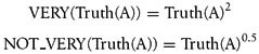
Here, Truth(A) is the degree of membership of A in some fuzzy set. Hedges effectively change the shape of membership functions. For example, these hedges applied to piecewise linear membership functions will result in the linear portions of those membership functions becoming nonlinear.
Hedges are not required in fuzzy systems. You can construct membership functions to suit your needs without the additional hedges. We mention them here for completeness, as they often appear in fuzzy logic literature.
Fuzzy Rules
After fuzzifying all input variables for a given problem, what we’d like to do next is construct a set of rules, combining the input in some logical manner, to yield some output. In an if-then style rule such as if A then B, the “if A” part is called the antecedent, or the premise. The “then B” part is called the consequent, or conclusion. We want to combine fuzzy input variables in a logical manner to form the premise, which will yield a fuzzy conclusion. The conclusion effectively will be the degree of membership in some predefined output fuzzy set.
Fuzzy Axioms
If we’re going to write logical rules given fuzzy input, we’ll need a way to apply the usual logical operators to fuzzy input much like we would do for Boolean input. Specifically, we’d like to be able to handle conjunction (logical AND), disjunction (logical OR), and negation (logical NOT). For fuzzy variables, these logical operators typically are defined as follows:
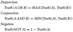
Here, again, Truth(A) means the degree of membership of A in some fuzzy set. This will be a real number between 0 and 1. The same applies for Truth(B) as well. As you can see, the logical OR operator is defined as the maximum of the operands, the AND operator is defined as the minimum of the operands, and NOT is simply 1 minus the given degree of membership.
Let’s consider an example. Given a person is overweight to a degree of 0.7 and tall to a degree of 0.3, the logical operators defined earlier result in the following:
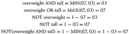
In code, these logical operations are fairly trivial, as shown in Example 10-1.
double FuzzyAND(double A, double B) {
   	return MIN(A, B);
}
double FuzzyOR(double A, double B) {
   	return MAX(A, B);
}
double FuzzyNOT(double A) {
   	return 1.0 - A;
}
These are not the only definitions used for AND, OR, and NOT. Some specific applications use other definitions—for example, you can define AND as the product of two degrees of membership, and you can define OR as the probabilistic-OR, as follows:
Some third-party fuzzy logic tools even facilitate user-defined logical operators, making the possibilities endless. For most applications, however, the definitions presented here work well.
Rule Evaluation
In a traditional Boolean logic application, rules such as if A AND B then C evaluate to absolutely true or false 1 or 0. After reading the previous section, you can see that this clearly is not the case using fuzzy logic. A AND B in fuzzy logic can evaluate to any number between 0 and 1, inclusive. This fact makes a fundamental difference in how fuzzy rules are evaluated versus Boolean logic rules.
In a traditional Boolean system, each rule is evaluated in series until one evaluates to true and it fires, so to speak—that is, its conclusion is processed. In a fuzzy rules system, all rules are evaluated in parallel. Each rule always fires; however, they fire to various degrees, or strengths. The result of the logical operations in each rule’s premise yields the strength of the rule’s conclusion. In other words, the strength of each rule represents the degree of membership in the output fuzzy set.
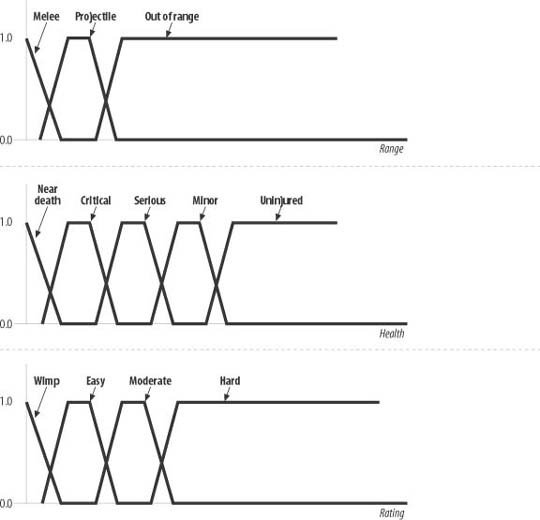
Let’s say you have a video game and are using a fuzzy system to evaluate whether a creature should attack a player. The input variables are range, creature health, and opponent ranking. The membership functions for each variable might look something like those shown in Figure 10-10.
The output actions in this example can be flee, attack, or do nothing. We can write some rules that look something like the following:
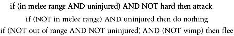
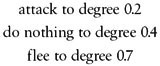
You can set up several more rules to handle more possibilities. In your game, all these rules would be evaluated to yield a degree of membership for each output action. Given specific degrees for the input variables, you might get outputs that look something like this:
In code, evaluation of these rules would look something like that shown in Example 10-1, where you can see a distinct difference from traditional if-then style rules.
degreeAttack = MIN(MIN (degreeMelee, degreeUninjured),
                               1.0 - degreeHard);
degreeDoNothing = MIN ( (1.0 - degreeMelee),
                               degreeUninjured);
degreeFlee = MIN (MIN ((1.0 - degreeOutOfRange),
                              (1.0 - degreeUninjured)),
                              (1.0 - degreeWimp));
The output degrees represent the strength of each rule. The easiest way to interpret these outputs is to take the action associated with the highest degree. In this example, the resulting action would be to flee.
In some cases, you might want to do more with the output than execute the action with the highest degree. For example, in the threat assessment case we discussed earlier in this chapter, you might want to use the fuzzy output to determine the number, a crisp number, of defensive units to deploy. To get a crisp number as an output, you have to defuzzify the results from the fuzzy rules.
Defuzzification
Defuzzification is required when you want a crisp number as output from a fuzzy system. As we mentioned earlier, each rule results in a degree of membership in some output fuzzy set. Let’s go back to our previous example. Say that instead of determining some finite action—do nothing, flee, or attack—you also want to use the output to determine the speed to which the creature should take action. For example, if the output action is to flee, does the creature walk away or run away, and how fast does it go? To get a crisp number, we need to aggregate the output strengths somehow and we need to define output membership functions.
For example, we might have output membership functions such as those shown in Figure 10-11.
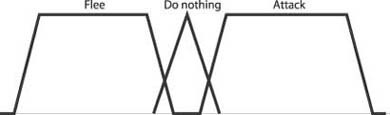
With the numerical output we discussed already—0.2 degree attack, 0.4 degree do nothing, and 0.7 degree flee—we’d end up with a composite membership function, as shown in Figure 10-12.
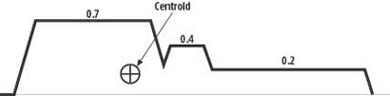
To arrive at such a composite membership function, each output set is truncated to the output degree of membership for that set as determined by the strength of the rules. Then all output sets are combined using disjunction.
At this point, we still have only an output membership function and no single crisp number. We can arrive at a crisp number from such an output fuzzy set in many ways. One of the more common methods involves finding the geometric centroid of the area under the output fuzzy set and taking the corresponding horizontal axis coordinate of that center as the crisp output. This yields a compromise between all the rules—that is, the single output number is a weighted average of all the output memberships.
To find the center of area for such an output function, you have to integrate the area under the curve using numerical techniques. Or you can consider it a polygon and use computational geometry methods to find the center. There are other schemes as well. In any case, finding the center of area is computationally expensive, especially considering the large number of times such a calculation would be performed in a game. Fortunately, there’s an easier way that uses so-called singleton output membership functions.
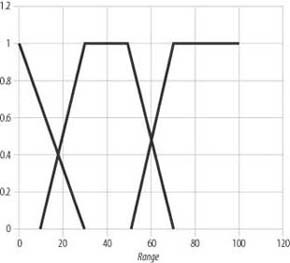
A singleton output function is really just a spike and not a curve. It is essentially a predefuzzified output function. For our example, we can assign speeds to each output action, such as -10 for flee, 1 for do nothing, and 10 for attack. Then, the resulting speed for flee, for example, would be the preset value of -10 times the degree to which the output action flee is true. In our example, we’d have -10 times 0.7, or -7 for the flee speed. (Here, the negative sign simply indicates flee as opposed to attack.) Considering the aggregate of all outputs requires a simple weighted average rather than a center of gravity calculation.
In general, let μ be the degree to which an output set is true and let x be the crisp result, singleton, associated with the output set. The aggregate, defuzzified output would then be:
In our example, we might have something such as:
Such an output when used to control the motion of the creature would result in the creature fleeing, but not necessarily in earnest.
To reinforce all the concepts we’ve discussed so far, let’s consider a few examples in greater detail.
Control Example
In the control example at the beginning of this chapter we wanted to use fuzzy control to steer a computer-controlled unit toward some objective. This objective could be a waypoint, an enemy unit, and so on. To achieve this, we’ll set up several fuzzy sets that describe the relative heading between the computer-controlled unit and its objective. The relative heading is simply the angle between the computer-controlled unit’s velocity vector and the vector connecting the positions of the computer-controlled unit and the objective. Using techniques we’ve discussed in earlier examples—namely, the chase and evade examples—you can determine this relative heading angle, which will be a scalar angle in degrees.
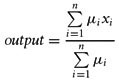
What we now aim to do is use that relative heading as input to a fuzzy control system to determine the appropriate amount of steering force to apply to guide the computer-controlled unit to the target. This is a very simple example, as there is only one input variable and thus only one set of fuzzy membership functions to define. For this example, we set up the membership functions and fuzzy sets illustrated in Figure 10-13.
We have five fuzzy sets in this case. Reading from left to right, each set represents relative headings qualitatively as Far Left, Left, Ahead, Right, and Far Right. The Far Left and Far Right membership functions are grade functions, while the Left and Right functions are trapezoids. The Ahead function is a triangle. Given any relative heading angle, you can use the C functions shown in Example 10-1 to calculate membership in each fuzzy set.
Let’s say that at some given time in the game, the relative heading angle is found to be a positive 33 degrees. Now we need to calculate the degree to which this relative heading falls within each of the five fuzzy sets. Clearly, the degree will be 0 for all sets, with the exception of the Right and Far Right sets. However, we’ll go ahead and show code for all membership calculations for completeness. Example 10-1 shows the code.
mFarLeft     =   FuzzyReverseGrade(33, -40, -30);
mLeft        =   FuzzyTrapezoid(33, -40, -25, -15, 0);
mAhead       =   FuzzyTriangle(33, -10, 10);
mRight       =   FuzzyTrapezoid(33, 0, 15, 25, 40);
mFarRight    =   FuzzyGrade(33, 30, 40);
In this example, the variables mFarLeft, mLeft, and so on, store the degree of membership of the relative heading value of 33 degrees in each predefined fuzzy set. The results are summarized in Table 10-1.
|
Fuzzy Set |
Degree of Membership |
|
Far Left |
0.0 |
|
Left |
0.0 |
|
Ahead |
0.0 |
|
Right |
0.47 |
|
Far Right |
0.3 |
Now, to use these resulting degrees of membership to control our unit, we’re going to simply apply each degree as a coefficient in a steering force calculation. Let’s assume that the maximum left steering force is some constant, FL, and the maximum right steering force is another constant, FR. We’ll let FL − 100 pounds of force, and FR = 100 pounds of force. Now we can calculate the total steering force to apply, as shown in Example 10-1.
NetForce= mFarLeft * FL + mLeft * FL + mRight * FR + mFarRight * FR;
The result of this calculation is 77 pounds of steering force. Notice that we didn’t include mAhead in the calculation. This means that any membership in Ahead does not require steering action. Technically, we could have done away with the Ahead membership function; however, we put it in there for emphasis.
In a physics-based simulation such as the examples we saw earlier in this book, this steering force would get applied to the unit for the cycle through the game loop within which the relative heading was calculated. The action of the steering force would change the heading of the unit for the next cycle through the game loop and a new relative heading would be calculated. This new relative heading would be processed in the same manner as discussed here to yield a new steering force to apply. Eventually the resultant steering force would smoothly decrease as the relative heading goes to 0. Or in fuzzy terms, as the degree of membership in the Ahead set goes to 1.
Threat Assessment Example
In the threat assessment example we discussed at the beginning of this chapter, we wanted to process two input variables, enemy force and the size of force, to determine the level of threat posed by this force. Ultimately, we want to determine the appropriate number for defensive units to deploy as protection against the threatening force. This example requires us to set up several fuzzy rules and defuzzify the output to obtain a crisp number for the number of defensive units to deploy. The first order of business, however, is to define fuzzy sets for the two input variables. Figures 10-14 and 10-15 show what we’ve put together for this example.
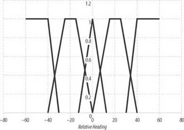
Referring to Figure 10-14 and going from the left to the right, these three membership functions represent the sets Close, Medium, and Far. The range can be specified in any units appropriate for your game. Let’s assume here that the range is specified in hexes.
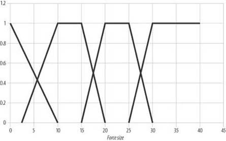
Referring to Figure 10-15 and going from left to right, these membership functions represent the fuzzy sets Tiny, Small, Moderate, and Large. With these fuzzy sets in hand, we’re ready to perform some calculations.
Let’s assume that during a given cycle through the game loop this fuzzy system is called upon to assess the threat posed by an enemy force eight units strong at a range of 25 hexes. So, now we need to fuzzify these crisp input values, determining the degree to which these variables fall within each predefined fuzzy set. Example 10-1 shows the code for this step.
mClose      = FuzzyTriangle(25, -30, 0, 30);
mMedium     = FuzzyTrapezoid(25, 10, 30, 50, 70);
mFar        = FuzzyGrade(25, 50, 70);
mTiny       = FuzzyTriangle(8, -10, 0, 10);
mSmall      = FuzzyTrapezoid(8, 2.5, 10, 15, 20);
mModerate   = FuzzyTrapezoid(8, 15, 20, 25, 30);
mLarge      = FuzzyGrade(8, 25, 30);
The results for this example are summarized in Table 10-2.
|
Fuzzy Set |
Degree of Membership |
|
Close |
0.17 |
|
Medium |
0.75 |
|
Far |
0.0 |
|
Tiny |
0.2 |
|
Small |
0.73 |
|
Moderate |
0.0 |
|
Large |
0.0 |
Before we consider any rules, let’s address output actions. In this case, we want the fuzzy output to be an indication of the threat level posed by the approaching force. We’ll use singleton output functions in this example, and the output, or action, fuzzy sets Low, Medium, and High for the threat level. Let’s define the singleton output values for each set to be 10 units, 30 units, and 50 units to deploy for Low, Medium, and High, respectively.
Now we can address the rules. The easiest way to visualize the rules in this case is through the use of a table, such as Table 10-3.
|
Close |
Medium |
Far | |
|
Tiny |
Medium |
Low |
Low |
|
Small |
High |
Low |
Low |
|
Moderate |
High |
Medium |
Low |
|
Large |
High |
High |
Medium |
The top row represents the range fuzzy sets, while the first column represents the force size fuzzy sets. The remaining cells in the table represent the threat level given the conjunction of any combination of range and force size. For example, if the force size is Tiny and the range is Close, the threat level is Medium.
We can set up and process the rules in this case in a number of ways. By inspecting Table 10-3, it’s clear that we can combine the input variables using various combinations of the AND and OR operators to yield one rule for each output set. However, this will result in rather unwieldy code with many nested logical operations. At the other extreme we can process one rule for each combination of input variables and pick the highest degree for each output set; however, this results in a bunch of rules. Nonetheless, it’s the simplest, most readable way to proceed, so we’ll sort of take that approach here. To simplify things further, we’ll show only combinations of input sets with nonzero degrees of membership, and we’ll make at least one nested operation. These are illustrated in Example 10-1.
.
.
.
mLow = FuzzyOr(FuzzyAND(mMedium, mTiny), FuzzyAND(mMedium, mSmall));
mMedium = FuzzyAND(mClose, mTiny);
mHigh = FuzzyAND(mClose, mSmall);
.
.
.
For our example, the results of these rule evaluations are mLow = 0.73, mMedium = 0.17, and mHigh = 0.17. These are the degrees of membership in the respective output fuzzy sets. Now we can defuzzify the results using the singleton output membership functions we defined earlier to get a single number representing the number of defensive forces to deploy. This calculation is simply a weighted average, as discussed earlier. Example 10-1 shows the code for this example.
nDeploy = ( mLow * 10 + mMedium * 30 + mHigh * 50) /
             (mLow + mMedium + mHigh);
The resulting number of units to deploy, nDeploy, comes to 19.5 units, or 20 if you round up. This seems fairly reasonable given the small size of the force and their proximity. Of course, all of this is subject to tuning. For example, you easily can adjust the results by changing the singleton values we used in this example. Also, the shapes of the various input membership functions are good candidates for tuning—you can try different shapes for each fuzzy set or use more or fewer fuzzy sets. Once everything is tuned, you’ll find that no matter what input values go in, the response always will vary smoothly from one set of input variables to another. Further, the results will be much harder for the player to predict because there are no clearly defined cutoffs, or breakpoints, at which the number of units to deploy would change sharply. This makes for much more interesting gameplay.