Because the examples we discuss rely heavily on generating random numbers, let’s look at some code to generate random numbers. The standard C function to generate a random number is rand(), which generates a random integer in the range from 0 to RAND_MAX. Typically RAND_MAX is set to 32727. To get a random integer between 0 and 99, use rand() % 100. Similarly, to get a random number between 0 and any integer N-1, use rand() % N. Don’t forget to seed the random number generator once at the start of your program by calling srand (seed). Note that srand takes a single unsigned int parameter as the random seed with which to initialize the random number generator.

In a very simple example, say you decide to program a little randomness to unit movement in your game. In this case, you can say the unit, when confronted, will move left with a 25% probability or will move right with a 25% probability or will back up with a 50% probability. Given these probabilities, you need only generate a random number between 0 and 99 and perform a few tests to determine in which direction to move the unit. To perform these tests, we’ll assign the range 0 to 24 as the possible range of values for the move-left event. Similarly, we’ll assign the range of values 75 to 99 as the possible range of values for the move-right event. Any other value between 25 and 74 (inclusive) indicates the backup event. Once a random number is selected, we need only test within which range it falls and then make the appropriate move. Admittedly, this is a very simple example, and one can argue that this is not intelligent movement; however, developers commonly use this technique to present some uncertainty to the player, making it more difficult to predict where the unit will move when confronted.

Another common use of probabilities in games involves representing a creature or player’s chances to hit an opponent in combat. Typically, the game developer defines several probabilities, given certain characteristics of the player and his opponent. For example, in a role-playing game you can say that a player with a moderate dexterity ranking has a 60% probability of striking his opponent with a knife in melee combat. If the player’s dexterity ranking is high, you might give him better odds of successfully striking with a knife; for example, you can say he has a 90% chance of striking his opponent. Notice that these are essentially conditional probabilities. We’re saying that the player’s probability of success is 90% given that he is highly dexterous, whereas his probability of success is 60% given that he is moderately dexterous. In a sense, all probabilities are conditional on some other event or events, even though we might not explicitly state the condition or assign a probability to it, as we did formally in the previous section. In fact, it’s common in games to make adjustments to such hit probabilities given other factors. For example, you can say that the player’s probability of successfully striking his opponent is increased to 95% given that he possesses a “dagger of speed.” Or, you can say the player’s chances of success are reduced to 85% given his opponent’s magic armor. You can come up with any number of these and list them in what commonly are called hit probability tables to calculate the appropriate probability given the occurrence or nonoccurrence of any number of enumerated events.

Yet another example of using probabilities in games is to define abilities of character classes or creature types. For example, say you have a role-playing game in which the player can take on the persona of a wizard, fighter, rouge, or ranger. Each class has its own strengths and weaknesses relative to the other classes, which you can enumerate in a table of skills with probabilities assigned so as to define each class’s characteristics. Table 12-1 gives a simple example of such a character class ability table.

Typically such character class tables are far more expansive than the few skills we show here. However, these serve to illustrate that each skill is assigned a probability of success, which is conditional on the character class. For example, a wizard has a 90% chance of successfully using magic, a fighter has a mere 5% chance, and so on. In practice these probabilities are further conditioned on the overall class level for each individual player. For example, a first-level wizard might have only a 10% chance of using magic. Here, the idea is that as the player earns levels, his proficiency in his craft will increase and the probabilities assigned to each skill will reflect this progress.

On the computer side of such a game’s AI, all creatures in the world will have similar sets of probability tables defining their abilities given their type. For example, dragons would have a different set of proficiencies than would giant apes, and so on.

You can take creature abilities a step further by combining probabilities with state transitions in the finite state machine that you can use to manage the various creature states. (See Chapter 9 for a discussion of finite state machines.) For example, Figure 12-1 illustrates a few states that a creature can assume.

Figure 12-1. Creature states

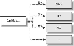
Let’s assume that this is one branch within a finite state machine that will be executed when the computer-controlled creature encounters the player. In the figure, Conditions are the necessary conditions that are checked in the finite state machine that would cause this set of states—Attack, Flee, Hide, etc.—to be considered. A condition could be something such as “the player is within range and has a weapon drawn.” Instead of deterministically selecting a state for the creature, we can assign certain probabilities to each applicable state. For illustration purposes we show that there’s a 50% chance the creature will attack the player. However, there’s a 20% chance the creature will flee the scene, and there’s a 10% chance it will try to hide. For even more variability, you can assign different probabilities to different types of creatures, making some more or less aggressive than others, and so on. Furthermore, within each creature type you can assign individual creatures different probabilities, giving each one their own distinct personality.

To select a state given probabilities such as these, you pick a random number between, say, 0 and 99, and check to see if it falls within specific ranges corresponding to each probability. Alternatively, you can take a lottery-type approach. In this case, you enumerate each state—for example, 0 for attack, 1 for flee, 2 for hide, and so on—and fill an array with these values in proportion to their probability. For example, for the attack state you’d fill half of the array with 0s. Once the array is populated, you simply pick a random number from 0 to the maximum size of the array minus 1, and you use that as an index to the array to get the chosen state.

A somewhat more compelling use of probability in games involves updating certain probabilities as the game is played in an effort to facilitate computer-controlled unit learning or adapting. For example, during a game you can collect statistics on the number and outcomes of confrontations between a certain type of creature and a certain class of player—for example, a wizard, fighter, and so on. Then you can calculate in real time the probability that the encounter results in the creature’s death. This is essentially the relative frequency approach to determining probabilities. Once you have this probability, you can use it—rather, the creature can—when deciding whether to engage players of this class in combat. If the probability is high that a certain class of player will kill this type of creature, you can have creatures of this type start to avoid that particular class. On the other hand, if the probability suggests that the creature might do well against a particular type of player class, you can have the creature seek out players of that class.

We look at this type of analysis in the next chapter, where we show you how to calculate such things as given the probability that the player is of a certain class and the probability that death results from encounters with this class, what is the probability that death will result? You could take this a step further by not assuming that the creature knows in what class the player belongs. Instead, the creature’s knowledge of the player can be uncertain, and it will have to infer what class he is facing to make a decision. Being able to collect statistics during gameplay and use probabilities for decisions clearly offers some interesting possibilities.

So far we discussed probability without actually giving it a formal definition. We need to do so before we move on to the next chapter on Bayesian methods. Further, we need to establish several fundamental rules of probability that you must know to fully appreciate the material in the next chapter. Therefore, in the remainder of this chapter we cover fundamental aspects of probability theory. If you’re already up to speed on this material, you can skip right to the next chapter.

Classical probability is an interpretation of probability that refers to events and possibilities, or possible outcomes. Given an event, E, which can occur in n ways out of a total of N possible outcomes, the probability, p, of occurrence of the event is:

Here, P(E) is the probability of event E, which is equal to the number of ways E occurs out of N possible ways. P(E) usually is called the probability of success of the event. The probability of failure of the event is 1-P(E). In summary:

Note that probabilities range in value from 0 to 1 and the sum of the probabilities of success and failure, p _s + p _f, must equal 1.

Let’s consider a simple example. Say you roll a six-sided die; the probability that a four will show up is 1/6 because there’s only one way in which a four can show up out of six possible outcomes in a single roll. In this example, the event, E, is the event that a four will show up. For the roll of a single die, a four can show up in only one way; therefore, n = 1. The total number of possible outcomes, N, is six in this case; therefore, P(E = 4) = 1/6. Clearly, in this case the probability of any given number showing up is 1/6 because each number can show up in only one possible way out of six ways.

Now, consider two six-sided dice, both rolled at the same time. What is the probability that the sum of the numbers that show up is equal to, say, five? Here, the event we’re interested in is a sum of five being rolled. In this case, there are four possible ways in which the sum of five can result. These are illustrated in Figure 12-2.

Figure 12-2. Sums of five in roll of two dice

Note that the outcome of the first die showing a two and the second showing a three is distinctly different from the outcome of the first die showing a three and the second showing a two. In this case, N = 36—that is, there are 36 possible outcomes of the roll of two dice. The probability, then, that the sum of five will appear is four divided by 36, with 36 being the total number of possible outcomes for two six-sided dice. This results in a probability of 4/36 or 1/9.

You can find the probability that any sum can show up in a similar manner. For example, the possible ways in which the sum of seven can occur are summarized in Table 12-2.

In this case, the probability of a sum of seven is 6/36 or 1/6. Stated another way, the probability of a sum of seven is 16.7%. We can express probability as percentages by taking the probability value, which will be between 0 and 1, and multiplying it by 100.

The frequency interpretation of probability, also known as relative frequency or objective probability, considers events and samples or experiments. If an experiment is conducted N times and some event, E, occurs n times, the probability of E occurring is:

Note here the caveat that P(E) is n/N as the number of experiments conducted gets very large. For a finite number of experiments, the resulting probability will be approximate, or empirical, because it is derived statistically. Empirical probability can be slightly different from theoretical probability if it can, indeed, be calculated for a given event. Additionally, we’re assuming the experiments are independent—that is, the outcome of one experiment does not affect the outcome of any other experiment.

Consider a simple experiment in which a coin is tossed 1000 times. The results of this experiment show that heads came up 510 times. Therefore, the probability of getting heads is 510/1000, which yields:

Of course, in this example we know that P(heads) is 0.5 or 50% and were we to continue with these experiments for a larger number of tosses we would expect our empirically derived P(heads) to approach 0.5.

Subjective probability is a measure, on a scale from zero to one, of a person’s degree of belief that a particular event will occur given their knowledge, experience, or judgment. This interpretation is useful when the event, or experiment, in question is not repeatable—that is, we can’t use a frequency measure to calculate a probability.

Subjective probabilities are found everywhere—we can say “it probably will rain tomorrow” or “I have a good chance of passing this test” or “the Saints probably will win tomorrow.” In each case, we base our belief in the outcome of these events on our knowledge of the events, whether it is complete or incomplete knowledge, and on our judgment considering a potential variety of relevant factors. For example, the fact that it is raining today might lead us to believe that it probably will rain tomorrow. We believe the Saints might win tomorrow’s football game with a better-than-usual probability because we know the other team’s star quarterback is suffering from an injury.

Consider this example: let’s assume you’re up for the lead game designer promotion in your company. You might say, “I have a 50% chance of getting the promotion,” knowing that someone else in your group with identical qualifications also is being considered for the job. One the other hand, you might say, “I have about a 75% chance of getting the promotion,” knowing that you’ve been with this company longer than your colleague who also is being considered. If in this case you also learn that the other candidate has notoriously missed milestone deadlines on various game projects, you might be inclined to revise your belief that you’ll get the promotion to something like a 90% chance. Formally, Bayesian analysis enables us to update our belief of some event given such new information. We discuss this in much greater detail in the next chapter.

Subjective probabilities very often are difficult to pin down, even when one has a fairly good intuitive feeling about a particular event. For example, if you say you probably will pass that test, what would you say is the actual probability: 60%, 80%, or 90%? You can employ some techniques to help pin down subjective probabilities, and we go over two of them shortly. Before we do that, however, we need to cover two other fundamental topics: odds and expectation.

Odds

Odds show up commonly in betting scenarios. For example, Sunflower Petals might be the long shot to win next week’s horse race, and the odds against her winning are 20 to 1; a football fan might take 3 to 1 odds on a bet in favor of the Giants winning Sunday’s game; and so on. For many, it’s easier or more intuitive to think of probabilities in terms of odds rather than in terms of some number between 0 and 1, or in terms of percentages. Odds reflect probabilities, and you can convert between them using a few simple relations.

If we say the odds in favor of the success of some event, E, are a to b, the probability of success of that event, P(E), is:

We can work in the other direction from probability to odds too. If you are given the probability of success of some event, P(E), the odds in favor of the event succeeding are P(E) to (1-P(E)). For example, if the odds are 9 to 1 that you’ll pass a test, the probability that you’ll pass is 0.9 or 90%. If, however, the probability you’ll pass is only 0.6, or 60%, because you didn’t study as much as you would have liked, the odds in favor of you passing are 60 to 40 or 1.5 to 1.

Expectation

Often it is useful in probability problems to think in terms of expectation. Mathematical expectation is the expected value of some discrete random variable, X, that can take on any values, x ₀, x ₁, x ₂, …, x _n, with corresponding probabilities, p ₀, p ₁, p ₂, …, p _n. You calculate the expectation for such a distribution of outcomes as follows:

For distributions such as this, you can think of the expectation as an average value. Statisticians think of expectation as a measure of central tendency. Decision theorists think of expectation as some measure of payoff.

As a very simple example, if you stand to win $100 with a probability of 0.12, your expectation is $12—that is, $100 times 0.12.

As another example, say you have a perpetual online role-playing game in which you monitor the number of players who gather at the local tavern each evening. Let’s assume from this monitoring you establish the probabilities shown in Table 12-3 for the number of players in the tavern each evening. Let’s further assume that the samples you used to calculate these frequency-based probabilities were all taken at about the same time of day; for example, you might have a spy casing the tavern every night collecting intelligence for an upcoming invasion.

Table 12-3. Probabilities of number of players in tavern each evening

# Players	Probability
0	0.02
2	0.08
4	0.20
6	0.24
8	0.17
10	0.13
12	0.10
14	0.05
16	0.01

Note that this distribution forms a mutually exclusive, exhaustive set. That is, there can’t be, say, zero and eight players there at the same time—it has to be one or the other—and the sum of probabilities for all these outcomes must be equal to 1. In this case, the expectation, the expected number of players in the tavern in the evening, is equal to 7.1. You can calculate this by taking the sum of the products of each pair of numbers appearing in each row of the table. Therefore, in any given evening, one can expect to find about seven players in the tavern, on average. Note that using this kind of analysis, an invading force could estimate how many units to send toward the tavern to take control of it.

Techniques for Assigning Subjective Probability

As we stated earlier, it is often very difficult to pin subjective probabilities to a specific number. Although you might have a good feel for the probability of some event, you might find it difficult to actually assign a single number to the probability of that event. To help in this regard, several commonly used metaphors are available to assist you in assigning numbers to subjective probabilities. We briefly discuss two of them here.

The first technique we can use to assign subjective probabilities is a betting metaphor. Let’s return to the promotion example we discussed earlier. Let’s say that another co-worker asked if you’re willing to make a wager on whether you’ll get the promotion. If the co-worker takes the side that you won’t get the promotion and is willing to put up $1 on the bet, but then asks for 9 to 1 odds, you’ll have to pay $9 if you lose and you’ll gain $1 if you win. Would you accept this bet? If you would, you consider this a fair bet and you essentially are saying you believe you’ll get the promotion with a probability of 90%. You can calculate this by considering the odds to which you agreed and using the relationship between odds and probability we discussed earlier. If you rejected these odds but instead offered 4 to 1 odds in favor of you getting the promotion, you essentially are saying you believe the probability that you’ll get the promotion is 4/5 or 80%.

Underlying this approach is the premise that you believe that the agreed-upon odds constitute a fair bet. Subjectively, a fair bet is one in which the expected gain is 0 and it does not matter to you which side of the bet you choose. Let’s say you took the 9 to 1 odds and you thought this was a fair bet. In this case, you expect to win ($1)(0.9) or 90 cents. This is simply the amount you will win times the probability that you will win. At the same time you expect to lose ($9)(0.1) or 90 cents—the amount you are wagering times the probability that you will lose. Therefore, the net gain you expect is your expected winnings minus your expected loss, which is clearly 0. Now, if you took this bet with 9 to 1 odds, but you really felt that your probability of successfully getting the promotion was only 80% as compared to 90%, your expected gain would be:

In this case you’d expect to lose $1, which indicates that this would not be a fair bet.

The betting metaphor we described here is the so-called put up or shut up approach in which you’re required to really think about the probability in terms of what you’d be willing to wager on the outcome. The idea is that you should get a pretty good sense of your true belief about a particular outcome.

There’s a problem with this approach, however, that is due to individual tolerances for risk. When we’re talking about $1 versus $9, the idea of losing $9 might not be that significant to you and you might have a greater propensity to take these odds. However, what if the bets were $100 and $900, or perhaps even $1000 and $9000? Certainly, most rational people who don’t own a money tree would think a little harder about their belief in some outcome occurring when larger sums of money are at stake. In some cases, the risk of losing so much money would override their belief in a certain outcome occurring, even if their subjective probability were well founded. And therein lies the problem in using this technique when perceived risk becomes significant: a person’s subjective probability could be biased by the risk they perceive.

An alternative to the betting metaphor is the so-called fair price metaphor whereby instead of betting on the outcome of an event, you ask yourself to put a fair price on some event. For example, let’s consider an author of a book who stands to earn $30,000 in royalties if the book he wrote is successful. Further, suppose that he will get nothing if the book fails. Now suppose the author is given the option by his publisher of taking an upfront, guaranteed payment of $10,000, but if he accepts he forfeits any further royalty rights. The question now is, what is the author’s subjective probability, his belief, that the book will be successful?

If the author accepts the deal, we can infer that $10,000 is greater than his expectation—that is, $10,000 ≥ ($30,000)(p), where p is his assigned subjective probability of the book’s success. Therefore, in this case his belief that the book will be successful as expressed by p is less than 0.33 or 33%. To get this we simply solve for p—that is, p ≥ $10,000/$30,000. If the author rejects the deal, he evidently feels the book has greater than a 33% chance of success—that is, his expectation is greater than $10,000.

To narrow down what the author feels the probability of success of the book actually is, we can simply ask him what he would take up front—we ask him what he thinks is a fair price for the rights to the book. From his reply we can calculate the subjective probability that he has assigned for the book’s success using the formula for expectation as before. If U is the amount he would accept up front, the subjective probability of the book’s success, p, is simply U/$30,000.

You can come up with various versions of this fair-price metaphor yourself depending on for what it is you’re trying to estimate a subjective probability. The idea here is to eliminate any bias that might be introduced when considering scenarios in which your own money is at risk, as in the betting technique.

This rule states the probability of an event, P(A), must be a real number between 0 and 1, inclusive. This rule serves to constrain the range of values assigned to probabilities. On one end of the scale we can’t have a negative probability, while on the other end the probability of an event can’t be greater than 1, which implies absolute certainty that the event will occur.

As sort of an extension of rule 1, if S represents the entire sample space for the event, the probability of S equals 1. This says that because the sample space includes all possible outcomes, there is a 100% probability that one of the outcomes therein will occur. Here, it helps to visualize the sample space and events using Venn diagrams. Figure 12-3 illustrates a Venn diagram for the sample space S and events A and B within that sample space.

Figure 12-3. Venn diagram

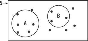
The dots represent samples taken within the space, and the relative sizes of the circles for A and B indicate their relative probabilities—more specifically, their areas indicate their probabilities.

If the probability that an event, A, will occur is P(A) and the event that A will not occur is designated A’, the probability of the event not occurring, P(A'), is 1- P(A). This rule simply states that an event either occurs or does not occur and the probability of this event either occurring or not occurring is 1—that is, we can say with certainty the event either will occur or will not occur. Figure 12-4 illustrates events A and Aapos; on a Venn diagram.

Figure 12-4. P(A) versus P(A')

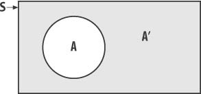
Clearly, event Aapos; covers all of the area within the sample space S that falls outside of event A.

This rule states that if two events A and B are mutually exclusive, only one of them can occur at a given time. For example, in a game, the events creature is dead and creature is alive are mutually exclusive. The creature cannot be both dead and alive at the same time. Figure 12-5 illustrates two mutually exclusive events A and B.

Figure 12-5. Mutually exclusive events

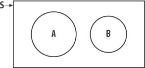
Note that the areas representing these two events do not overlap. For two mutually exclusive events, A and B, the probability of event A or event B occurring is as follows:

where P(A ∪ B) is the probability of event A or event B, the probability that one or the other occurs, and P(A) and P(B) are the probabilities of events A and B, respectively.

You can generalize this rule for more than two mutually exclusive events. For example, if A, B, C, and D are four mutually exclusive events, the probability that A or B or C or D occurs is:

Theoretically you can generalize this to any number of mutually exclusive events.

This rule states that if the events under consideration are not mutually exclusive, we need to revise the formulas discussed in rule 4. For example, in a game a given creature can be alive, dead, or injured. Although alive and dead are mutually exclusive, alive and injured are not. The creature can be alive and injured at the same time. Figure 12-6 shows two nonmutually exclusive events.

Figure 12-6. Nonmutually exclusive events

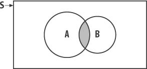
In this case, the areas for events A and B overlap. This means that event A can occur or event B can occur or both events A and B can occur simultaneously. The shaded area in Figure 12-5 indicates the probability that both A and B occur together. Therefore, to calculate the probability of event A or event B occurring in this case, we use the following formula:

In this formula, P(A ∪ B) is the probability that both A and B occur.

You also can generalize this formula to more than two nonmutually exclusive events. Figure 12-7 illustrates three events, A, B, and C, that are not mutually exclusive.

Figure 12-7. Three nonmutually exclusive events

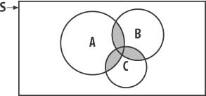
To calculate the probability of A or B or C we need to calculate the probability corresponding to the shaded region in Figure 12-7. The formula that achieves this is as follows:

This rule states that if two events, A and B, are independent—that is, the occurrence of one event does not depend on the occurrence or nonoccurrence of the other event—the probability of events A and B both occurring is as follows:

For example, two independent events in a game can be player encounters a wandering monster and player is building a fire. The occurrence of either of these events is independent of the occurrence of the other event. Now consider another event, player is chopping wood. In this case, the event player encounters a wandering monster might very well depend on whether the player is chopping wood. These events are not independent. By chopping wood, the player presumably is in a forest, which increases the likelihood of him encountering a wandering monster.

Referring to Figure12-6, this probability corresponds to the shaded region shared by events A and B.

If events A and B are not independent, we must deal with the so-called conditional probability of these events. The preceding formula does not apply in the conditional case. The rule governing conditional probabilities is so important, especially in the context of Bayesian analysis, we’re going to discuss it next in its own section.