As we said earlier, the simplest chase algorithm involves correcting the predator’s coordinates based on the prey’s coordinates so as to reduce the distance between their positions. This is a very common method for implementing basic chasing and evading. (In this method, evading is virtually the opposite of chasing, whereby instead of trying to decrease the distance between the predator and prey coordinates, you try to increase it.) In code, the method looks something like that shown in Example 2-1.

if (predatorX > preyX)
     predatorX--;
else if (predatorX < preyX)
     predatorX++;
if (predatorY > preyY)
     predatorY--;
else if (predatorY < preyY)
     predatorY++;

In this example, the prey is located at coordinates preyX and preyY, while the predator is located at coordinates predatorX and predatorY. During each cycle through the game loop the predator’s coordinates are checked against the prey’s. If the predator’s x-coordinate is greater than the prey’s x-coordinate, the predator’s x-coordinate is decremented, moving it closer to the prey’s x-position. Conversely, if the predator’s x-coordinate is less than the prey’s, the predator’s x-coordinate is incremented. Similar logic applies to the predator’s y-coordinate based on the prey’s y-coordinate. The end result is that the predator will move closer and closer to the prey each cycle through the game loop.

Using this same methodology, we can implement evading by simply reversing the logic, as we illustrate in Example 2-2.

if (preyX > predatorX)
     preyX++;
else if (preyX < predatorX)
     preyX--;
if (preyY > predatorY)
     preyY++;
else if (preyY < predatorY)
     preyY--;

In tile-based games the game domain is divided into discrete tiles—squares, hexagons, etc.—and the player’s position is fixed to a discrete tile. Movement goes tile by tile, and the number of directions in which the player can make headway is limited. In a continuous environment, position is represented by floating-point coordinates, which can represent any location in the game domain. The player also is free to head in any direction.

You can apply the approach illustrated in these two examples whether your game incorporates tile-based or continuous movement. In tile-based games, the xs and ys can represent columns and rows in a grid that encompasses the game domain. In this case, the xs and ys would be integers. In a continuous environment, the xs and ys—and zs if yours is a 3D game—would be real numbers representing the coordinates in a Cartesian coordinate system encompassing the game domain.

There’s no doubt that although it’s simple, this method works. The predator will chase his prey with unrelenting determination. The sample program AIDemo2-1, available for download from this book’s web site (http://www.oreilly.com/ai), implements the basic chase algorithm in a tile-based environment. The relevant code is shown in Example 2-3.

if (predatorCol > preyCol)
     predatorCol--;
else if (predatorCol < preyCol)
     predatorCol++;
if (predatorRow> preyRow)
     predatorRow--;
else if (predatorRow<preyRow)
     predatorRow++;

Notice the similarities in Examples 2-3 and 2-1. The only difference is that in Example 2-3 rows and columns are used instead of floating-point xs and ys.

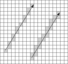
The trouble with this basic method is that often the chasing or evading seems almost too mechanical. Figure 2-1 illustrates the path the troll in the sample program takes as he pursues the player.

Figure 2-1. Basic tile-based chase

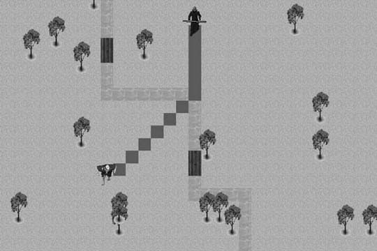
As you can see, the troll first moves diagonally toward the player until one of the coordinates, the horizontal in this case, equals that of the player’s.^[2] Then the troll advances toward the player straight along the other coordinate axis, the vertical in this case. Clearly this does not look very natural. A better approach is to have the troll move directly toward the player in a straight line. You can implement such an algorithm without too much difficulty, as we discuss in the next section.

^[2]

In this section we explain a few chasing and evading algorithms that use a line-of-sight approach. The gist of the line-of-sight approach is to have the predator take a straight-line path toward the prey; the predator always moves directly toward the prey’s current position. If the prey is standing still, the predator will take a straight line path. However, if the prey is moving, the path will not necessarily be a straight line. The predator still will attempt to move directly toward the current position of the prey, but by the time he catches up with the moving prey, the path he would have taken might be curved, as illustrated in Figure 2-2.

Figure 2-2. Line-of-sight chasing

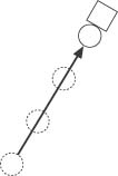
In Figure 2-2, the circles represent the predator and the diamonds represent the prey. The dashed lines and shapes indicate starting and intermediate positions. In the scenario on the left, the prey is sitting still; thus the predator makes a straight-line dash toward the prey. In the scenario on the right, the prey is moving along some arbitrary path over time. At each time step, or cycle through the game loop, the predator moves toward the current position of the prey. As the prey moves, the predator traces out a curved path from its starting point.

The results illustrated here look more natural than those resulting from the basic-chase algorithm. Over the remainder of this section, we’ll show you two algorithms that implement line-of-sight chasing. One algorithm is specifically for tiled environments, while the other applies to continuous environments.

As we stated earlier, the environment in a tile-based game is divided into discrete tiles. This places certain limitations on movement that don’t necessarily apply in a continuous environment. In a continuous environment, positions usually are represented using floating-point variables. Those positions are then mapped to the nearest screen pixel. When changing positions in a continuous environment, you don’t always have to limit movement to adjacent screen pixels. Screen pixels typically are small enough so that a small number of them can be skipped between each screen redraw without sacrificing motion fluidity.

In tile-based games, however, changing positions is more restrictive. By its very nature, tile-based movement can appear jaggy because each tile is not mapped to a screen pixel. To minimize the jaggy and sometimes jumpy appearance in tile-based games, it’s important to move only to adjacent tiles when changing positions. For games that use square tiles, such as the example game, this offers only eight possible directions of movement. This limitation leads to an interesting problem when a predator, such as the troll in the example, is chasing its target. The troll is limited to only eight possible directions, but mathematically speaking, none of those directions can accurately represent the true direction of the target. This dilemma is illustrated in Figure 2-3.

Figure 2-3. Tile-based eight-way movement

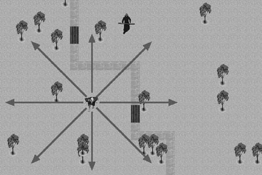
As you can see in Figure 2-3, none of the eight possible directions leads directly to the target. What we need is a way to determine which of the eight adjacent tiles to move to so that the troll appears to be moving toward the player in a straight line.

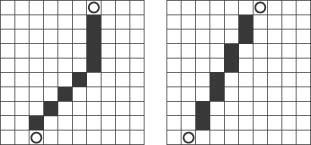
As we showed you earlier, you can use the simple chasing algorithm to make the troll relentlessly chase the player. It will even calculate the shortest possible path to the player. So, what’s the disadvantage? One concerns aesthetics. When viewed in a tile-based environment, the simple chase method doesn’t always appear to produce a visually straight line. Figure 2-4 illustrates this point.

Figure 2-4. Simple chase versus line-of-sight chase

Another reason to avoid the simple chase method is that it can have undesirable side effects when a group of predators, such as a pack of angry trolls, are converging on the player. Using the simple method, they would all walk diagonally to the nearest axis of their target and then walk along that axis to the target. This could lead to them walking single file to launch their attack. A more sophisticated approach is to have them walk directly toward the target from different directions.

It’s interesting to note that both paths shown in Figure 2-4 are the same distance. The line-of-sight method, however, appears more natural and direct, which in turn makes the troll seem more intelligent. So, the objective for the line-of-sight approach is to calculate a path so that the troll appears to be walking in a straight line toward the player.

The approach we’ll take to solve this problem involves using a standard line algorithm that is typically used to draw lines in a pixel environment. We’re essentially going to treat the tile-based environment as though each tile was in fact a giant screen pixel. However, instead of coloring the pixels to draw a line on the screen, the line algorithm is going to tell us which tiles the troll should follow so that it will walk in a straight line to its target.

Although you can calculate the points of a line in several ways, in this example we’re going to use Bresenham’s line algorithm. Bresenham’s algorithm is one of the more efficient methods for drawing a line in a pixel-based environment, but that’s not the only reason it’s useful for pathfinding calculations. Bresenham’s algorithm also is attractive because unlike some other line-drawing algorithms, it will never draw two adjacent pixels along a line’s shortest axis. For our pathfinding needs, this means the troll will walk along the shortest possible path between the starting and ending points. Figure 2-5 shows how Bresenham’s algorithm, on the left, might compare to other line algorithms that can sometimes draw multiple pixels along the shortest axis. If an algorithm that generated a line such as the one shown on the right is used, the troll would take unnecessary steps. It still would still reach its target, but not in the shortest and most efficient way.

Figure 2-5. Bresenham versus alternate line algorithm

As Figure 2-5 shows, a standard algorithm such as the one shown on the right would mark every tile for pathfinding that mathematically intersected the line between the starting and ending points. This is not desirable for a pathfinding application because it won’t generate the shortest possible path. In this case, Bresenham’s algorithm produces a much more desirable result.

The Bresenham algorithm used to calculate the direction of the troll’s movement takes the starting point, which is the row and column of the troll’s position, and the ending point, which is the row and column of the player’s position, and calculates a series of steps the troll will have to take so that it will walk in a straight line to the player. Keep in mind that this function needs to be called each time the troll’s target, in this case the player, changes position. Once the target moves, the precalculated path becomes obsolete, and therefore it becomes necessary to calculate it again. Examples 2-4 through 2-7 show how you can use the Bresenham algorithm to build a path to the troll’s target.

void ai_Entity::BuildPathToTarget (void)
{
     int nextCol=col;
     int nextRow=row;
     int deltaRow=endRow-row;
     int deltaCol=endCol-col;
     int stepCol, stepRow;
     int currentStep, fraction;

As Example 2-4 shows, this function uses values stored in the ai_Entity class to establish the starting and ending points for the path. The values in col and row are the starting points of the path. In the case of the sample program, col and row contain the current position of the troll. The values in endRow and endCol contain the position of the troll’s desired location, which in this case is the player’s position.

for (currentStep=0;currentStep<kMaxPathLength; currentStep++)
{
    pathRow[currentStep]=-1;
        pathCol[currentStep]=-1;
}
currentStep=0;
pathRowTarget=endRow;
pathColTarget=endCol;

In Example 2-5 you can see the row and column path arrays being initialized. This function is called each time the player’s position changes, so it’s necessary to clear the old path before the new one is calculated.

Upon this function’s exit, the two arrays, pathRow and pathCol, will contain the row and column positions along each point in the troll’s path to its target. Updating the troll’s position then becomes a simple matter of traversing these arrays and assigning their values to the troll’s row and column variables each time the troll is ready to take another step.

Had this been an actual line-drawing function, the points stored in the path arrays would be the coordinates of the pixels that make up the line.

The code in Example 2-6 determines the direction of the path by using the previously calculated deltaRow and deltaCol values.

     if (deltaRow <  0) stepRow=-1;  else stepRow=1;
     if (deltaCol <  0) stepCol=-1;  else stepCol=1;
     deltaRow=abs(deltaRow*2);
     deltaCol=abs(deltaCol*2);
     pathRow[currentStep]=nextRow;
     pathCol[currentStep]=nextCol;
     currentStep++;

It also sets the first values in the path arrays, which in this case is the row and column position of the troll.

Example 2-7 shows the meat of the Bresenham algorithm.

if (deltaCol >deltaRow)
      {
       fraction = deltaRow *2-deltaCol;
       while (nextCol != endCol)
        {
         if (fraction >=0)
          {
           nextRow =nextRow +stepRow;
           fraction =fraction -deltaCol;
          }
         nextCol=nextCol+stepCol;
         fraction=fraction +deltaRow;
         pathRow[currentStep]=nextRow;
         pathCol[currentStep]=nextCol;
         currentStep++;
        }
      }
     else
      {
       fraction =deltaCol *2-deltaRow;
       while (nextRow !=endRow)
        {
         if (fraction >=0)
          {
           nextCol=nextCol+stepCol;
           fraction=fraction -deltaRow;
          }
         nextRow =nextRow +stepRow;
         fraction=fraction +deltaCol;
         pathRow[currentStep]=nextRow;
         pathCol[currentStep]=nextCol;
         currentStep++;
        }
       }
      }

The initial if conditional uses the values in deltaCol and deltaRow to determine which axis is the longest. The first block of code after the if statement will be executed if the column axis is the longest. The else part will be executed if the row axis is the longest. The algorithm will then traverse the longest axis, calculating each point of the line along the way. Figure 2-6 shows an example of the path the troll would follow using the Bresenham line-of-sight algorithm. In this case, the row axis is the longest, so the else part of the main if conditional would be executed.

Figure 2-6. Bresenham tile-based chase

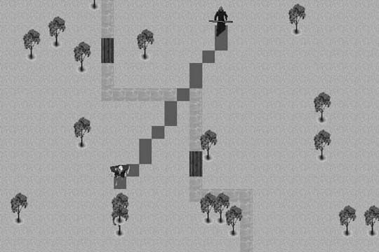
Figure 2-6 shows the troll’s path, but of course this function doesn’t actually draw the path. Instead of drawing the line points, this function stores each row and column coordinate in the pathRow and pathCol arrays. These stored values are then used by an outside function to guide the troll along a path that leads to the player.

The Bresenham algorithm is an effective method for tiled environments. In this section we discuss a line-of-sight chase algorithm in the context of continuous environments. Specifically, we will show you how to implement a simple chase algorithm that you can use for games that incorporate physics engines where the game entities—airplanes, spaceships, hovercraft, etc.—are driven by applied forces and torques.

The example we’ll discuss in this section uses a simple two-dimensional, rigid-body physics engine to calculate the motion of the predator and prey vehicles. You can download the complete source code for this sample program, AIDemo2-2, from this book’s web site. We’ll cover as much rigid-body physics as necessary to get through the example, but we won’t go into great detail. For thorough coverage of this subject, refer to Physics for Game Developers (O’Reilly).

Here’s the scenario. The player controls his vehicle by applying thrust for forward motion and steering forces for turning. The computer-controlled vehicle uses the same mechanics as the player’s vehicle does, but the computer controls the thrust and steering forces for its vehicle. We want the computer to chase the player wherever he moves. The player will be the prey while the computer will be the predator. We’re assuming that the only information the predator has about the prey is the prey’s current position. Knowing this, along with the predator’s current position, enables us to construct a line of sight from the predator to the prey. We will use this line of sight to decide how to steer the predator toward the prey. (In the next section we’ll show you another method that assumes knowledge of the player’s position and velocity expressed as a vector.)

Before getting to the chase algorithm, we want to explain how the predator and prey vehicles will move. The vehicles are identical in that both are pushed about by some applied thrust force and both can turn via activation of steering forces. To turn right, a steering force is applied that will push the nose of the vehicle to the right. Likewise, to turn left, a steering force is applied that will push the nose of the vehicle to the left. For the purposes of this example, we assume that the steering forces are bow thrusters—for example, they could be little jets located on the front end of the vehicle that push the front end to either side. These forces are illustrated in Figure 2-7.

Figure 2-7. Vehicle forces

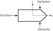
The line-of-sight algorithm will control activation of the steering forces for the predator so as to keep it heading toward the prey at all times. The maximum speed and turning rate of each vehicle are limited due to development of linear and angular drag forces (forces that oppose motion) that are calculated and applied to each vehicle. Also, the vehicles can’t always turn on a dime. Their turning radius is a function of their linear speed—the higher their linear speed, the larger the turning radius. This makes the paths taken by each vehicle look smoother and more natural. To turn on a dime, they have to be traveling fairly slowly.

Example 2-8 shows the function that controls the steering for the predator. It gets called every time step through the simulation—that is, every cycle through the physics engine loop. What’s happening here is that the predator constantly calculates the prey’s location relative to itself and then adjusts its steering to keep itself pointed directly toward the prey.

void    DoLineOfSightChase (void)
{
     Vector   u, v;
     bool     left = false;
     bool     right = false;
     u = VRotate2D(-Predator.fOrientation,
                        (Prey.vPosition - Predator.vPosition));
     u.Normalize();
     if (u.x <  -_TOL)
          left = true;
     else if (u.x > _TOL)
          right = true;
     Predator.SetThrusters(left, right);
}

As you can see, the algorithm in Example 2-8 is fairly simple. Upon entering the function, four local variables are defined. u and v are Vector types, where the Vector class is a custom class (see Appendix A) that handles all the basic vector math such as vector addition, subtraction, dot products, and cross products, among other operations. The two remaining local variables are a couple of boolean variables, left and right. These are flags that indicate which steering force to turn on; both are set to false initially.

The next line of code after the local variable definitions calculates the line of sight from the predator to the prey. Actually, this line does more than calculate the line of site. It also calculates the relative position vector between the predator and prey in global, earth-fixed coordinates via the code (Prey.vPosition - Predator.vPosition), and then it passes the resulting vector to the function VRotate2D to convert it to the predator’s local, body-fixed coordinates. VRotate2D performs a standard coordinate-system transform given the body-fixed coordinate system’s orientation with respect to the earth-fixed system (see the sidebar “Global & Local Coordinate Systems”). The result is stored in u, and then u is normalized—that is, it is converted to a vector of unit length.

Global & Local Coordinate Systems

A global (earth-fixed) coordinate system is fixed and does not move, whereas a local (body-fixed) coordinate system is locked onto objects that move around within the global, fixed coordinate system. A local coordinate system also rotates with the object to which it is attached.

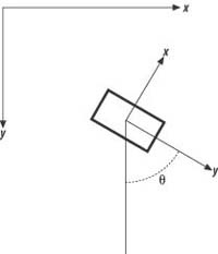
You can use the following equations to convert coordinates expressed in terms of global coordinates to an object’s local coordinate system given the object’s orientation relative to the global coordinate system:

Here, (x, y) are the local, body-fixed coordinates of the global point (X, Y).

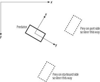
What we have now is a unit vector, u, pointing from the predator directly toward the prey. With this vector the next few lines of code determine whether the prey is to the port side, the starboard side, or directly in front of the predator, and steering adjustments are made accordingly. The local y-axis fixed to the predator points in the positive direction from the back to the front of the vehicle—that is, the vehicle always heads along the positive local y-axis.

So, if the x-position of the prey, in terms of the predator’s local coordinate system, is negative, the prey is somewhere to the starboard side of the predator and the port steering force should be activated to correct the predator’s heading so that it again points directly toward the prey. Similarly, if the prey’s x-coordinate is positive, it is somewhere on the port side of the predator and the starboard steering force should be activated to correct the predator’s heading. Figure 2-8 illustrates this test to determine which bow thruster to activate. If the prey’s x-coordinate is zero, no steering action should be taken.

Figure 2-8. Steering force test

The last line of code calls the SetThrusters member function of the rigid body class for the predator to apply the steering force for the current iteration through the simulation loop. In this example we assume a constant steering force, which can be tuned as desired.

The results of this algorithm are illustrated in Figure 2-9.

Figure 2-9. Line-of-sight chase in continuous environment

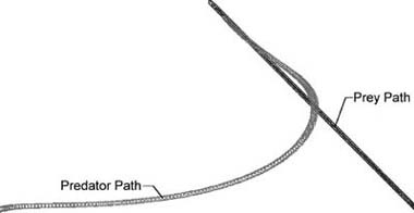
Figure 2-9 shows the paths taken by both the predator and the prey. At the start of the simulation, the predator was located in the lower left corner of the window while the prey was located in the lower right. Over time, the prey traveled in a straight line toward the upper left of the window. The predator’s path curved as it continuously adjusted its heading to keep pointing toward the moving prey.

Just like the basic algorithm we discussed earlier in this chapter, this line-of-sight algorithm is relentless. The predator will always head directly toward the prey and most likely end up right behind it, unless it is moving so fast that it overshoots the prey, in which case it will loop around and head toward the prey again. You can prevent overshooting the prey by implementing some sort of speed control logic to allow the predator to slow down as it gets closer to the prey. You can do this by simply calculating the distance between the two vehicles, and if that distance is less than some predefined distance, reduce the forward thrust on the predator. You can calculate the distance between the two vehicles by taking the magnitude of the difference between their position vectors.

If you want the computer-controlled vehicle to evade the player rather than chase him, all you have to do is reverse the greater-than and less-than signs in Example 2-8.

The line-of-sight chase algorithm we discussed in the previous section in the context of continuous movement is effective in that the predator always will head directly toward the prey. The drawback to this algorithm is that heading directly toward the prey is not always the shortest path in terms of range to target or, perhaps, time to target. Further, the line-of-sight algorithm usually ends up with the predator following directly behind the prey unless the predator is faster, in which case it will overshoot the prey. A more desirable solution in many cases—for example, a missile being shot at an aircraft—is to have the predator intercept the prey at some point along the prey’s trajectory. This allows the predator to take a path that is potentially shorter in terms of range or time. Further, such an algorithm could potentially allow slower predators to intercept faster prey.

To explain how the intercept algorithm works, we’ll use as a basis the physics-based game scenario we described earlier. In fact, all that’s required to transform the basic- chase algorithm into an intercept algorithm is the addition of a few lines of code within the chase function. Before getting to the code, though, we want to explain how the intercept algorithm works in principle. (You can apply the same algorithm, building on the line-of-sight example we discussed earlier, in tile-based games too.)

The basic idea of the intercept algorithm is to be able to predict some future position of the prey and to move toward that position so as to reach it at the same time as the prey. This is illustrated in Figure 2-10.

Figure 2-10. Interception

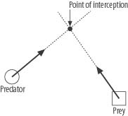
At first glance it might appear that the predicted interception point is simply the point along the trajectory of the prey that is closest to the location of the predator. This is the shortest-distance-to-the-line problem, whereby the shortest distance from a point to the line is along a line segment that is perpendicular to the line. This is not necessarily the interception point because the shortest-distance problem does not consider the relative velocities between the predator and the prey. It might be that the predator will reach the shortest-distance point on the prey’s trajectory before the prey arrives. In this case the predator will have to stop and wait for the prey to arrive if it is to be intercepted. This obviously won’t work if the predator is a projectile being fired at a moving target such as an aircraft. If the scenario is a role-playing game, as soon as the player sees that the predator is in his path, he’ll simply turn away.

To find the point where the predator and prey will meet at the same time, you must consider their relative velocities. So, instead of just knowing the prey’s current position, the predator also must know the prey’s current velocity—that is, its speed and heading. This information will be used to predict where the prey will be at some time in the future. Then, that predicted position will become the target toward which the predator will head to make the interception. The predator must then continuously monitor the prey’s position and velocity, along with its own, and update the predicted interception point accordingly. This facilitates the predator changing course to adapt to any evasive maneuvers the prey might make. This, of course, assumes that the predator has some sort of steering capability.

At this point you should be asking how far ahead in time you should try to predict the prey’s position. The answer is that it depends on the relative positions and velocities of both the predator and the prey. Let’s consider the calculations involved one step at a time.

The first thing the predator must do is to calculate the relative velocity between itself and the prey. This is called the closing velocity and is simply the vector difference between the prey’s velocity and the predator’s:

Here the relative, or closing, velocity vector is denoted V _r. The second step involves calculating the range to close. That’s the relative distance between the predator and the prey, which is equal to the vector difference between the prey’s current position and the predator’s current position:

Here the relative distance, or range, between the predator and prey is denoted S _r. Now there’s enough information to facilitate calculating the time to close.

The time to close is the average time it will take to travel a distance equal to the range to close while traveling at a speed equal to the closing speed, which is the magnitude of the closing velocity, or the relative velocity between the predator and prey. The time to close is calculated as follows:

The time to close, t _c, is equal to the magnitude of the range vector, S _r, divided by the magnitude of the closing velocity vector, V _r.

Now, knowing the time to close, you can predict where the prey will be t _c in the future. The current position of the prey is S _prey and it is traveling at V _prey. Because speed multiplied by time yields average distance traveled, you can calculate how far the prey will travel over a time interval t _c traveling at V _prey and add it to the current position to yield the predicted position, as follows:

Here, S _t is the predicted position of the prey t _c in the future. It’s this predicted position, S _t, that now becomes the target, or aim, point for the predator. To make the interception, the predator should head toward this point in much the same way as it headed toward the prey using the line-of-sight chase algorithm. In fact, all you need to do is to add a few lines of code to Example 2-8, the line-of-sight chase function, to convert it to an intercepting function. Example 2-9 shows the new function.

void     DoIntercept(void)
{
     Vector   u, v;
     Bool     left = false;
     Bool     right = false;
     Vector   Vr, Sr, St;   // added this line
     Double   tc             // added this line
     // added these lines:
     Vr = Prey.vVelocity - Predator.vVelocity;
     Sr = Prey.vPosition - Predator.vPosition;
     tc = Sr.Magnitude() / Vr.Magnitude();
     St = Prey.vPosition + (Prey.vVelocity * tc);
     // changed this line to use St instead of Prey.vPosition:
     u = VRotate2D(-Predator.fOrientation,
                        (St - Predator.vPosition));
     // The remainder of this function is identical to the line-of-
     // sight chase function:
     u.Normalize();
     if (u.x <  -_TOL)
          left = true;
     else if (u.x > _TOL)
          right = true;
     Predator.SetThrusters(left, right);
}

The code in Example 2-9 is commented to highlight where we made changes to adapt the line-of-sight chase function shown in Example 2-8 to an intercept function. As you can see, we added a few lines of code to calculate the closing velocity, range, time to close, and predicted position of the prey, as discussed earlier. We also modified the line of code that calculates the target point in the predator’s local coordinates to use the predicted position of the prey rather than its current position.

That’s all there is to it. This function should be called every time through the game loop or physics engine loop so that the predator constantly updates the predicted interception point and its own trajectory.

The results of this algorithm as incorporated into example AIDemo2-2 are illustrated in Figures 2-11 through 2-14.

Figure 2-11. Intercept scenario 1—initial trajectories

Figure 2-12. Intercept scenario 1—interception

Figure 2-13. Intercept scenario 2—corrective action

Figure 2-14. Intercept scenario 2—interception

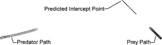
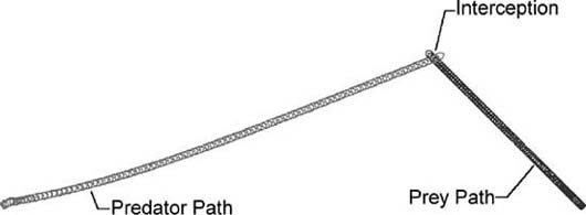
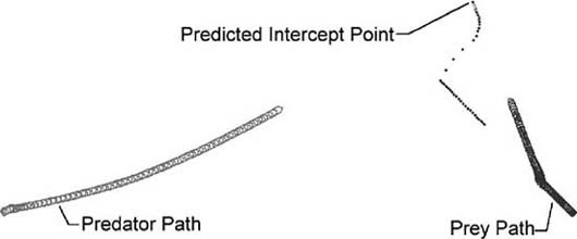
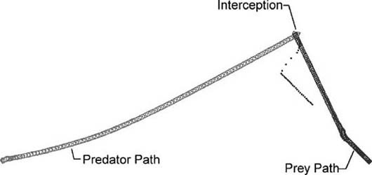
Figure 2-11 illustrates a scenario in which the predator and prey start out from the lower left and right corners of the window, respectively. The prey moves at constant velocity from the lower right to the upper left of the window. At the same time the predator calculates the predicted interception point and heads toward it, continuously updating the predicted interception point and its heading accordingly. The predicted interception point is illustrated in this figure as the streak of dots ahead of the prey. Initially, the interception point varies as the predator turns toward the prey; however, things settle down and the interception point becomes fixed because the prey is moving at constant velocity.

After a moment the predator intercepts the prey, as shown in Figure 2-12.

Notice the difference between the path taken by the predator using the intercept algorithm versus that shown in Figure 2-9 using the line-of-sight algorithm. Clearly, this approach yields a shorter path and actually allows the predator and prey to cross the same point in space at the same time. In the line-of-sight algorithm, the predator chases the prey in a roundabout manner, ending up behind it. If the predator was not fast enough to keep up, it would never hit the prey and might get left behind.

Figure 2-13 shows how robust the algorithm is when the prey makes some evasive maneuvers.

Here you can see that the initial predicted intercept point, as illustrated by the trail of dots ahead of the prey, is identical to that shown in Figure 2-11. However, after the prey makes an evasive move to the right, the predicted intercept point is immediately updated and the predator takes corrective action so as to head toward the new intercept point. Figure 2-14 shows the resulting interception.

The interception algorithm we discussed here is quite robust in that it allows the predator to continuously update its trajectory to effect an interception. After experimenting with the demo, you’ll see that an interception is made almost all the time.

Sometimes interceptions are not possible, however, and you should modify the algorithm we discussed here to deal with these cases. For example, if the predator is slower than the prey and if the predator somehow ends up behind the prey, it will be impossible for the predator to make an interception. It will never be able to catch up to the prey or get ahead of it to intercept it, unless the prey makes a maneuver so that the predator is no longer behind it. Even then, depending on the proximity, the prey still might not have enough speed to effect an interception.

In another example, if the predator somehow gets ahead of the prey and is moving at the same speed or faster than the prey, it will predict an interception point ahead of both the prey and the predator such that neither will reach the interception point—the interception point will constantly move away from both of them. In this case, the best thing to do is to detect when the predator is ahead of the prey and have the predator loop around or take some other action so as to get a better angle on the prey. You can detect whether the prey is behind the predator by checking the position of the prey relative to the predator in the predator’s local coordinate system in a manner similar to that shown in Examples 2-8 and 2-9. Instead of checking the x-coordinate, you check the y-coordinate, and if it is negative, the prey is behind the predator and the preditor needs to turn around. An easy way to make the predator turn around is to have it go back to the line-of-sight algorithm instead of the intercept algorithm. This will make the predator turn right around and head back directly toward the prey, at which point the intercept algorithm can kick back in to effect an interception.

Earlier we told you that chasing and evading involves two, potentially three, distinct problems: deciding to chase or evade, actually effecting the chase or evasion, and obstacle avoidance. In this chapter we discussed the second problem of effecting the chase or evasion from a few different perspectives. These included basic chasing, line-of-sight chasing, and intercepting in both tiled and continuous environments. The methods we examined here are effective and give an illusion of intelligence. However, you can greatly enhance the illusions by combining these methods with other algorithms that can deal with the other parts of the problem—namely, deciding when and if to chase or evade, and avoiding obstacles while in pursuit or on the run. We’ll explore several such algorithms in upcoming chapters.

Also, note that other algorithms are available for you to use to effect chasing or evading. One such method is based on the use of potential functions, which we discuss in Chapter 5.