
Chapter 14. Neural Networks
Our brains are composed of billions of neurons, each one connected to thousands of other neurons to form a complex network of extraordinary processing power. Artificial neural networks, hereinafter referred to simply as neural networks or networks, attempt to mimic our brain’s processing capability, albeit on a far smaller scale.
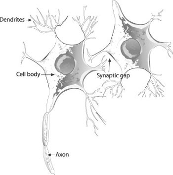
Information, so to speak, is transmitted from one neuron to another via the axon and dendrites. The axon carries the voltage potential, or action potential, from an activated neuron to other connected neurons. The action potential is picked up from receptors in the dendrites. The synaptic gap is where chemical reactions take place, either to excite or inhibit the action potential input to the given neuron. Figure 14-1 illustrates a neuron.
The adult human brain contains about 1011 neurons and each neuron receives synaptic input from about 104 other neurons. If the combined effect of all these inputs is of sufficient strength, the neuron will fire, transmitting its action potential to other neurons.
The artificial networks we use in games are quite simple by comparison. For many applications artificial neural networks are composed of only a handful, a dozen or so, neurons. This is far simpler than our brains. Some specific applications use networks composed of perhaps thousands of neurons, yet even these are simple in comparison to our brains. At this time we can’t hope to approach the processing power of the human brain using our artificial networks; however, for specific problems our simple networks can be quite powerful.
This is the biological metaphor for neural networks. Sometimes it’s helpful to think of neural networks in a less biological sense. Specifically, you can think of a neural network as a mathematical function approximator. Input to the network represents independent variables, while output represents the dependant variable(s). The network itself is a function giving one unique set of output for the given input. The function in this case is difficult to write in equation form and fortunately we don’t need to do so. Further, the function is highly nonlinear. We’ll come back to this way of thinking a little later.
For games, neural networks offer some key advantages over more traditional AI techniques. First, using a neural network enables game developers to simplify coding of complex state machines or rules-based systems by relegating key decision-making processes to one or more trained neural networks. Second, neural networks offer the potential for the game’s AI to adapt as the game is played. This is a rather compelling possibility and is a very popular subject in the game AI community at the time of this writing.
In spite of these advantages, neural networks have not gained widespread use in video games. Game developers have used neural networks in some popular games; but by and large, their use in games is limited. This probably is due to several factors, of which we describe two key factors next.
First, neural networks are great at handling highly nonlinear problems; ones you cannot tackle easily using traditional methods. This sometimes makes understanding exactly what the network is doing and how it is arriving at its results difficult to follow, which can be disconcerting for the would-be tester. Second, it’s difficult at times to predict what a neural network will generate as output, especially if the network is programmed to learn or adapt within a game. These two factors make testing and debugging a neural network relatively difficult compared to testing and debugging a finite state machine, for example.
Further, some early attempts at the use of neural networks in games have tried to tackle complete AI systems—that is, massive neural networks were assembled to handle the most general AI tasks that a given game creature or character could encounter. The neural network acted as the entire AI system—the whole brain, so to speak. We don’t advocate this approach, as it compounds the problems associated with predictability, testing, and debugging. Instead, just like our own brains have many areas that specialize in specific tasks, we suggest that you use neural networks to handle specific game AI tasks as part of an integrated AI system that uses traditional AI techniques as well. In this way, the majority of the AI system will be relatively predictable, and the hard AI tasks or the ones which you want to take advantage of learning and adapting will use specific neural networks that were trained strictly for that one task.
The AI community uses many different kinds of neural networks to solve all sorts of problems, from financial to engineering problems and many in between. Neural networks often are combined with other techniques such as fuzzy systems, genetic algorithms, and probabilistic methods, to name a few. This subject is far too vast to treat in a single chapter, so we’re going to narrow our focus on a particularly useful class of neural networks. We’re going to concentrate our attention on a type of neural network called a multilayer, feed-forward network. This type of network is quite versatile and is capable of handling a wide variety of problems. Before getting into the details of such a network, let’s first explore in general terms how you can apply neural networks in games.
Control
Neural networks often are used as neural controllers for robotics applications. In these cases, the robot’s sensory system provides relevant inputs to the neural controller, and the neural controller’s output, which can consist of one or more output nodes, sends the proper responses to the robot’s motor control system. For example, a neural controller for a robot tank might take three inputs, each indicating whether an obstacle is sensed in front of or to either side of the robot. (The range to each sensed obstacle also can be input.) The neural controller can have two outputs that control the direction of motion of its left and right tracks. One output node can set the left track to move forward or backward, while the other can set the right track to move forward or backward. The combination of the resulting outputs has the robot either move forward, move backward, turn left, or turn right. The neural network might look something such as that illustrated in Figure 14-2.
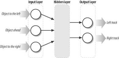
Very similar situations arise in games. You can, in fact, have a computer-controlled, half-track mechanized unit in your game. Or perhaps you want to use a neural network to handle the flight controls for a spaceship or aircraft. In each case, you’ll have one or more input neurons and one or more output neurons that will control the unit’s thrust, wheels, tracks, or whatever means of locomotion you’re simulating.
Threat Assessment
As another example, say you’re writing a strategy simulation-type game in which the player has to build technology and train units to fend off or attack the computer-controlled base. Let’s say you decide to use a neural network to give the computer-controlled army some means of predicting the type of threat presented by the player at any given time during gameplay. One possible neural network is illustrated in Figure 14-3.
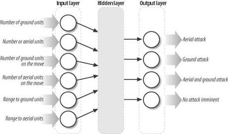
The inputs to this network include the number of enemy (the player) ground units, the number of enemy aerial units, an indication as to whether the ground units are on the move, an indication as to whether the aerial units are on the move, the range to the ground units, and the range to the aerial units. The outputs consist of neurons that indicate one of four possible threats, including an aerial threat, a ground threat, both an aerial and a ground threat, or no threat. Given appropriate data during gameplay and a means of assessing the performance of the network (we’ll talk about training later), you can use such a network to predict what, if any, sort of attack is imminent. Once the threat is assessed, the computer can take the appropriate action. This can include deployment of ground or aerial forces, shoring up defenses, putting foot soldiers on high alert, or carrying on as usual, assuming no threat.
This approach requires in-game training and validation of the network, but potentially can tune itself to the playing style of the player. Further, you are alleviated of the task of figuring out all the possible scenarios and thresholds if you were to use a rules-based or finite state machine-type architecture for this task.
Attack or Flee
As a final example, let’s say you have a persistent role-playing game and you decide to use a neural network to control how certain creatures in the game behave. Now let’s assume you’re going to use a neural network to handle the creature’s decision-making process—that is, whether the creature will attack, evade, or wander, depending on whether an enemy (a player) is in the creature’s proximity. Figure 14-4 shows how such a neural network might look. Note that you would use this network only to decide whether to attack, evade, or wander. You would use other game logic, such as the chasing and evading techniques we discussed earlier, to execute the desired action.
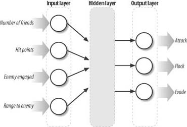
We have four inputs in this example: the number of like creatures in proximity to the creature who’s making the decision (this is an indication of whether the creature is traveling in a group or alone); a measure of the creature’s hit points or health; an indication as to whether the enemy is engaged in combat with another creature; and finally, the range to the enemy.
We can make this example a little more sophisticated by adding more inputs, such as the class of the enemy, whether the enemy is a mage or a fighter, and so on. Such a consideration would be important to a creature whose attack strategies and defenses are better suited against one type of class or another. You could determine the enemy’s class by “cheating,” or better yet, you could predict the enemy’s class by using another neural network or Bayesian analysis, adding a bit more uncertainty to the whole process.
Dissecting Neural Networks
In this section we’re going to dissect a three-layer feed-forward neural network, looking at each of its components to see what they do, why they are important, and how they work. The aim here is to clearly and concisely take the mystery out of neural networks. We’ll take a rather practical approach to this task and leave some of the more academic aspects to other books on the subject. We will give references to several such books throughout this chapter.
Structure
We focus on three-layer feed-forward networks in this chapter. Figure 14-5 illustrates the basic structure of such a network.
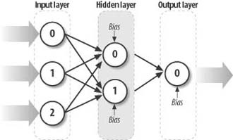
A three-layer network consists of one input layer, one hidden layer, and one output layer. There’s no restriction on the number of neurons within each layer. Every neuron from the input layer is connected to every neuron in the hidden layer. Further, every neuron in the hidden layer is connected to every neuron in the output layer. Also, every neuron, with the exception of the input layer, has an additional input called the bias. The numbers shown in Figure 14-5 serve to identify each node in the three layers. We’ll use this numbering system later when we write the formulas for calculating the value of each neuron.
Calculating the output value(s) for a network starts with some input provided to each input neuron. Then these inputs are weighted and passed along to the hidden-layer neurons. This process repeats, going from the hidden layer to the output layer, where the output of the hidden-layer neurons serves as input to the output layer. This process of going from input to hidden to output layer is the feed-forward process. We’ll look at each component of this type of network in more detail in the following sections.
Input
Inputs to a neural network obviously are very important; without them there’s nothing for the neural network to process. Clearly we need them, but what should you choose as inputs? How many do you need? And what form should they take?
Input: What and How Many?
The question of what to choose as input is very problem-specific. You have to look at the problem you’re trying to solve and select what game parameters, data, and environment characteristics are important to the task at hand. For example, say you’re designing a neural network to classify player characters in a role-playing game so that the computer-controlled creatures can decide whether they want to engage the player. Some inputs you might consider include some indication of the player’s attire, his drawn weapon if present, and perhaps any witnessed actions—for example, whether his just cast a spell.
Your job of training the neural network, which we’ll discuss later, will be easier if you keep the number of input neurons to a minimum. However, in some situations the inputs to select won’t always be obvious to you. In such cases, the general rule is to include what inputs you think might be important and let the neural network sort out for itself which ones are important. Neural networks excel at sorting out the relative importance of inputs to the desired output. Keep in mind, however, that the more inputs you throw in, the more data you’re going to have to prepare to train the network, and the more computations you’ll have to make in the game.
Often you can reduce the number of inputs by combining or transforming important information into some other, more compact form. As a simple example, let’s say you’re trying to use a neural network to control a spacecraft landing on a planet in your game. The mass of the spacecraft, which could be variable, and the acceleration due to gravity on the planet clearly are important factors, among others, that you should provide as input to the neural network. You could, in fact, create one input neuron for each parameter—one for the mass and another for the acceleration due to gravity. However, this approach forces the neural network to perform extra work in figuring out a relationship between the spacecraft’s mass and the acceleration due to gravity. A better input capturing these two important parameters is a single neuron that takes the weight of the spacecraft—the product of its mass times the acceleration due to gravity—as an input to a single neuron. There would, of course, be other input neurons besides this one, for example, you probably would have altitude and speed inputs as well.
Input: What Form?
You can use a variety of forms of data as inputs to a neural network. In games, such input generally consists of three types: boolean, enumerated, and continuous types. Neural networks work with real numbers, so whatever the type of data you have, it must be converted to a suitable real number for use as input.
Consider the example shown in Figure 14-4. The “enemy engaged” input is clearly a boolean type—true if the enemy is engaged and false otherwise. However, we can’t pass true or false to a neural network input node. Instead, we input a 1.0 for true and a 0.0 for false.
Sometimes your input data might be enumerated. For example, say you have a network designed to classify an enemy, and one consideration is the kind of weapon he is wielding. The choices might be something such as dagger, bastard sword, long sword, katana, crossbow, short bow, or longbow. The order does not matter here, and we assume that these possibilities are mutually exclusive. Typically you handle such data in neural networks using the so-called one-of-n encoding method. Basically, you create an input for each possibility and set the input value to 1.0 or 0.0 corresponding to whether each specific possibility is true. If, for example, the enemy was wielding a katana, the input vector would be {0, 0, 0, 1, 0, 0, 0} where the 1 is set for the katana input node and the 0s are set for all other possibilities.
Very often your data will, in fact, be a floating-point number or an integer. In either case this type of data generally can take on any number of values between some practical upper and lower bounds. You simply can input these values directly into the neural network (which game developers often do).
This can cause some problems, however. If you have input values that vary widely in terms of order of magnitude, the neural network might give more weight to the larger-magnitude input. For example, if one input ranges from 0 to 20 while another ranges from 0 to 20,000, the latter likely will swamp out the influence of the former. Thus, in these cases it is important to scale such input data to ranges that are comparable in terms of order of magnitude. Commonly, you can scale such data in terms of percentage values ranging from 0 to 100, or to values ranging from 0 to 1. Scaling in this way levels the playing field for the various inputs. You must be careful how you scale, however. You need to make sure the data used to train your network is scaled in the exact same way as the data the network will see in the field. For example, if you scale a distance input value by the screen width for your training data, you must use the same screen width to scale your input data when the network is functioning in your game.
Weights
Weights in a neural network are analogous to the synaptic connection in a biological neural network. The weights affect the strength of a given input and can be either inhibitory or excitatory. It is the weights that truly define the behavior of a neural network. Further, the task of determining the value of these weights is the subject of training or evolving a neural network.
Every connection from one neuron to another has an associated weight. This is illustrated in Figure 14-5. The input to a neuron is then the sum of the products of each input’s weight connecting that neuron times its input value plus a bias term, which we’ll discuss later. The net result is called the net input to a neuron. The following equation shows how the net input to a given neuron, neuron j, is calculated from a set of input, i, neurons.
Referring to Figure 14-5, you can see that every input to a neuron is multiplied by the weight of the connection between those two neurons plus the bias. Let’s look at a simple example (we’ll take a look at source code for these calculations later).
Let’s say we want to calculate the net input to the 0th neuron in the hidden layer shown in Figure 14-5. Applying the previous equation, we get the following formula for the net input to the 0th neuron in the hidden layer:
In this formula the ns represents the value of the neuron. In the case of the input neurons, these are the input values. In the case of the hidden neurons, they are the net input values. The superscripts h and i represent to which layer the neuron belongs—h for the hidden layer and i for the input layer. The subscripts indicate the node within each layer.
Notice here that the net input to a given neuron is simply a linear combination of weighted inputs from other neurons. If this is so, how does a neural network approximate highly nonlinear functions such as those we mentioned earlier? The key lies in how the net input is transformed to an output value for a neuron. Specifically, activation functions map the net input to a corresponding output in a nonlinear way.
Activation Functions
An activation function takes the net input to a neuron and operates on it to produce an output for the neuron. Activation functions should be nonlinear (except in one case, which we’ll discuss shortly). If they are not, the neural network is reduced to a linear combination of linear functions and is rendered incapable of approximating nonlinear functions and relationships.
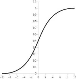
The most commonly used activation function is the logistic function or sigmoid function. Figure 14-6 illustrates this S-shaped function.
The formula for the logistic function is as follows:
Sometimes this functions is written in thes form:
In this case, the c term is used to alter the shape of the function—that is, either stretching or compressing the function along the horizontal axis.
Note that the input lies along the horizontal axis and the output from this function ranges from 0 to 1 for all values of x. In practice the working range is more like 0.1 to 0.9, where a value of around 0.1 implies the neuron is unactivated and a value of around 0.9 implies the neuron is activated. It is important to note that no matter how large (positive or negative) x gets, the logistic function will never actually reach 1.0 or 0.0; it asymptotes to these values. You must keep this in mind when training. If you attempt to train your network so that it outputs a value of 1 for a given output neuron, you’ll never get there. A more reasonable value is 0.9, and shooting for this value will speed up training immensely. The same applies if you are trying to train a network to output a value of 0. Use something such as 0.1 instead.
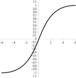
Other activation functions are at your disposal as well. Figures 14-7 and 14-8 show two other well-known activation functions: the step function and the hyperbolic tangent function.
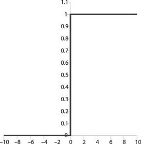
The formula for the step function is as follows:
Step functions were used in early neural network development, but their lack of a derivative made training tough. Note that the logistic function has an easy-to-evaluate derivative, which is needed for training the network, as we’ll see shortly.
The formula for the hyperbolic tangent function is as follows:
The hyperbolic tangent function is sometimes used and is said to speed up training. Other activation functions are used in neural networks for various applications; however, we won’t get into those here. In general, the logistic function seems to be the most widely used and is applicable to a large variety of applications.
Figure 14-9 shows yet another activation function that sometimes is used—a linear activation function.
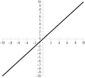
The formula for the linear activation function is simply:
This means that the output of a neuron is simply the net input—that is, the sum of the weighted inputs from all connected input neurons plus the bias term.
Linear activation functions sometimes are used as the activation functions for output neurons. Note that nonlinear activation functions must be used for the hidden neurons if the network is not to be reduced to a linear combination of linear functions. Employing such a linear output neuron is sometimes useful when you don’t want the output confined to an interval between 0 and 1. In such cases, you still can use a logistic output activation function, so long as you scale the output to the full range of values for which you’re interested.
Bias
When we discussed how to calculate the net input to a neuron earlier, we mentioned that each neuron has a bias associated with it. This is represented as a bias value and a bias weight for each neuron and shows up in the net input formula we showed earlier and are showing again here for convenience:
b j is the bias value and w j is the bias weight.
To understand what the bias does, you have to look at the activation functions used to generate output for a neuron given the net input. Basically, the bias term shifts the net input along the horizontal axis of the activation function, which effectively changes the threshold at which a neuron activates. The bias value always is set to 1 or −1 and its weight is adjusted through training, just like all other weights. This essentially allows the neural network to learn the appropriate thresholds for each neuron’s activation.
Some practitioners always set the bias value to 1, while others always use -1. In our experience it really doesn’t matter whether you use 1 or -1 because, through training, the network will adjust its bias weights to suit your choice. Weights can be either positive or negative, so if the neural network thinks the bias should be negative, it will adjust the weight to achieve that, regardless of your choice of 1 or -1. If you choose 1, it will find a suitable negative weight, whereas if you choose -1, it will find a suitable positive weight. Of course, you achieve all of this through training or evolving the network, as we’ll discuss later in this chapter.
Output
Just like input, your choice of output neurons for a given network is problem-specific. In general, it’s best to keep the number of output neurons to a minimum to reduce computation and training time.
Consider a network in which, given certain input, you desire output that classifies that input. Perhaps you want to determine whether a given set of input falls within a certain class. In this case, you would use one output neuron. If it is activated, the result is true, whereas if it is not activated, the result is false—the input does not fall within the class under consideration. If you were using a logistic function as your output activation, an output of around 0.9 would indicate activated, or true, whereas an output of around 0.1 would indicate not activated, or false. In practice, you might not actually get output values of exactly 0.9 or 0.1; you might get 0.78 or 0.31, for example. Therefore, you have to define a threshold that will enable you to assess whether a given output value indicates activation. Generally, you simply choose an output threshold midway between the two extremes. For the logistic function, you can use 0.5. If the output is greater than 0.5, the result is activated or true, otherwise it’s false.
When you’re interested in whether certain input falls within more than a single class, you have to use more than a single output neuron. Consider the network shown in Figure 14-3. Here, essentially we want to classify the threat posed by an enemy; the classes are aerial threat, ground threat, both aerial and ground threats, or no threat. We have one output neuron for each class. For this type of output we assume that high output values imply activated, while low output values imply not activated. The actual output values for each node can cover a range of values, depending on how the network was trained and on the kind of output activation function used. Given a set of input values and the resulting value at each output node, one way to figure out which output is activated is to take the neuron with the highest output value. This is the so-called winner-take-all approach. The neuron with highest activation indicates the resulting class. We’ll see an example of this approach later in this chapter.
Often, you want a neural network that will generate a single value given a set of input. Time-series prediction, whereby you try to predict the next value given historical values over time, is one such situation in which you’ll use a single output neuron. In this case, the value of the output neuron corresponds to the predicted value of interest. Keep in mind, however, you might have to scale the result if you’re using an output activation function that generates bounded values, such as the logistic function, and if the value of the quantity you’re trying to predict falls within some other range.
In other cases, such as that illustrated in Figure 14-2, you might have more than one output neuron that’s used to directly control some other system. In the case of the example shown in Figure 14-2, the output values control the motion of each track for a half-track robot. In that example, it might be useful to use the hyperbolic tangent function for the output neurons so that the output value will range between -1 and +1. Then, negative values could indicate backward motion while positive values could indicate forward motion.
Sometimes you might require a network with as many output neurons as input neurons. Such networks commonly are used for autoassociation (pattern recognition) and data compression. Here, the aim is that the output neurons should echo the input values. For pattern recognition, such a network would be trained to output its input. The training set would consist of many sample patterns of interest. The idea here is that when presented with a pattern that’s either degraded somewhat or does not exactly match a pattern that was included in the training set, the network should produce output that represents the pattern included in its training set that most closely matches the one being input.
The Hidden Layer
So far we’ve discussed input neurons, output neurons, and how to calculate net inputs for any neuron, but we’ve yet to discuss the hidden layer specifically. In our three-layer feed-forward network, we have one hidden layer of neurons sandwiched between the input and output layers.
As illustrated in Figure 14-5, every input is connected to every hidden neuron. Further, every hidden neuron sends its output to every output neuron. By the way, this isn’t the only neural network structure at your disposal; there are all sorts—some with more than one hidden layer, some with feedback, and some with no hidden layer at all, among others. However, it is one of the most commonly used configurations. At any rate, the hidden layer is crucial for giving the network facility to process features in the input data. The more hidden neurons, the more features the network can handle; conversely, the fewer hidden neurons, the fewer features the network can handle.
So, what do we mean by features? To understand what we mean here, it’s helpful to think of a neural network as a function approximator. Say you have a function that looks very noisy, as illustrated in Figure 14-10.

If you were to train a neural network to approximate such a function using too few hidden neurons, you might get something such as that shown in Figure 14-11.

Here, you can see that the approximated function captures the trend of the input data but misses the local noisy features. In some cases, such as for signal noise reduction applications, this is exactly what you want; however, you might not want this for other problems. If you go the other route and choose too many hidden neurons, the approximated function likely will pick up the local noisy features in addition to the overall trend of the function. In some cases, this might be what you want; however, in other cases, you might end up with a network that is overtrained and unable to generalize given new input data that was not part of the training set.
Exactly how many hidden neurons to use for a given application is hard to say with certainty. Generally, you go about it by trial and error. However, here’s a rule of thumb that you might find useful. For three-layer networks in which you’re not interested in autoassociation, the appropriate number of hidden neurons is approximately equal to the square root of the product of the number of input and output neurons. This is just an approximation, but it’s as good a place to start as any. The thing to keep in mind, particularly for games in which CPU usage is critical, is that the larger the number of hidden neurons, the more time it will take to compute the output of the network. Therefore, it’s beneficial to try to minimize the number of hidden neurons.
Training
So far, we’ve repeatedly mentioned training a neural network without actually giving you the details as to how to do this. We’ll tackle that now in this section.
The aim of training is to find the values for the weights that connect all the neurons such that the input data generates the desired output values. As you might expect, there’s more to training than just picking some weight values. Essentially, training a neural network is an optimization process in which you are trying to find optimal weights that will allow the network to produce the right output.
Training can fall under two categories: supervised training and unsupervised training. Covering all or even some of the popular training approaches is well beyond a single chapter, so we’ll focus on one of the most commonly used supervised training methods: back-propagation.
Back-Propagation Training
Again, the aim of training is to find the values for the weights that connect all the neurons such that the input data generates the desired output values. To do this, you need a training set, which consists of both input data and the desired output values corresponding to that input. The next step is to iteratively, using any of a number of techniques, find a set of weights for the entire network that causes the network to produce output matching the desired output for each set of data in the training set. Once you do this, you can put the network to work and present it with new data, not included in the training set, to produce output that is reasonable.
Because training is an optimization process, we need some measure of merit to optimize. In the case of back-propagation, we use a measure of error and try to minimize the error. Given some input and the generated output, we need to compare the generated output with the known, desired output and quantify how well the results match—i.e., calculate the error. Many error measures are available for you to use, and we’ll use one of the most common ones here: the mean square error, which is simply the average of the square of the differences between the calculated output and the desired output.
If you’ve studied calculus you might recall that to minimize or maximize a function you need to be able to calculate the function’s derivative. Because we’re trying to optimize weights by minimizing the error measure, it’s no surprise that we need to calculate a derivative somewhere. Specifically, we need the derivative of the activation function, and this is why the logistic function is so nice—we easily can determine its derivative analytically.
As we mentioned earlier, finding the optimum weights is an iterative process, and it goes something like this:
Start with a training set consisting of input data and corresponding desired outputs.
Initialize the weights in the neural network to some small random values.
With each set of input data, feed the network and calculate the output.
Compare the calculated output with the desired output and compute the error.
Adjust the weights to reduce the error, and repeat the process.
You can execute the process in two ways. One way is to calculate the error measure, adjust the weights for each set of input and desired output data, and then move on to the next set of input/output data. The other way is to calculate the cumulative error for all sets of input and desired output data in the training set, then adjust the weights, and then repeat the process. Each iteration is known as an epoch.
Steps 1 through 3 are relatively straightforward and we’ll see an example implementation a little later. Now, though, let’s examine steps 4 and 5 more closely.
Computing Error
To train a neural network, you feed it a set of input, which generates some output. To compare this calculated output to the desired output for a given set of input, you need to calculate the error. This enables you to not only determine whether the calculated output is right or wrong, but also to determine the degree to which it is right or wrong. The most common error to use is the mean-square error, which is the average of the square of the difference between the desired and calculated output:
In this equation, ∊ is the mean square error for the training set. n c and n d are the calculated and desired output values, respectively, for all output neurons, while m is the number of output neurons for each epoch.
The goal is to get this error value as small as is practical by iteratively adjusting the weight values connecting all the neurons in the network. To know how much the weights need adjusting, each iteration requires that we also calculate the error associated with each neuron in the output and hidden layers. We calculate the error for output neurons as follows:
Here, δ i o is the error for the i th output neuron, Δn i o is the difference between the calculated and desired output for the i th output neuron, and f′(nci o) is the derivative of the activation function for the i th output neuron. Earlier we told you that we’d need to calculate a derivative somewhere, and this is where to do it. This is why the logistic function is so useful; its derivative is quite simple in form, and it’s easy to calculate it analytically. Rewriting this equation using the derivative of the logistic function yields the following equation for output neuron error:
In this equation, n di o is the desired output value for the i th neuron, and n ci o is the calculated output value for the i th neuron.
For hidden-layer neurons, the error equation is somewhat different. In this case, the error associated with each hidden neuron is as follows:
Notice here that the error for each hidden-layer neuron is a function of the error associated with each output-layer neuron to which the hidden neuron connects times the weight for each connection. This means that to calculate the error and, subsequently, to adjust weight, you need to work backward from the output layer toward the input layer.
Also notice that the activation function derivative is required again. Assuming the logistic activation function yields the following:
Lastly, no error is associated with input layer neurons because those neuron values are given.
Adjusting Weights
With calculated errors in hand, you can proceed to calculate suitable adjustments for each weight in the network. The adjustment to each weight is as follows:
In this equation, ρ is the learning rate, δ i is the error associated with the neurons being considered, and n i is the value of the neuron being considered. The new weight is simply the old weight plus Δw.
Keep in mind that the weight adjustments will be made for each weight and the adjustment will be different for each weight. When updating the weights connecting output to hidden-layer neurons, the errors and values for the output neurons calculate the weight adjustment. When updating the weights connecting the hidden- to-input-layer neurons, the errors and values for the hidden-layer neurons are used.
The learning rate is a multiplier that affects how much each weight is adjusted. It’s usually set to some small value such as 0.25 or 0.5. This is one of those parameters that you’ll have to tune. If you set it too high, you might overshoot the optimum weights; if you set it too low, training might take longer.
Momentum
Many back-propagation practitioners use a slight modification to the weight adjustments we just discussed. This modified technique is called adding momentum. Before showing you how to add momentum, let’s first discuss why you might want to add momentum.
In any general optimization process the goal is to either minimize or maximize some function. More specifically, we’re interested in finding the global minimum or maximum of the given function over some range of input parameters. The trouble is that many functions exhibit what are called local minima or maxima. These are basically hollows and humps in the function, as illustrated in Figure 14-12.
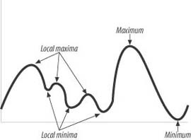
In this example, the function has a global minimum and maximum over the range shown; but it also has several local minima and maxima, characterized by the smaller bumps and hollows.
In our case, we’re interested in minimizing the error of our network. Specifically we’re interested in finding the optimum weights that yield the global minimum error; however, we might run into a local minimum instead of a global minimum.
When network training begins, we initialize the weights to some small random values. We have no idea at that point how close those values are to the optimum weights; thus, we might have initialized the network near a local minimum rather than a global minimum. Without going into calculus, the technique by which we update the weights is called a gradient descent type of technique, whereby we use the derivative of the function in an attempt to steer toward a minimum value, which in our case is a minimum error value. The trouble is that we don’t know if we get to a global minimum or a local minimum, and typically the error-space, as it’s called for neural networks, is full of local minima.
This sort of problem is common among all optimization techniques and many different methods attempt to alleviate it. The momentum technique is one such technique used for neural networks. It does not eliminate the possibility of converging on a local minimum, but it is thought to help get out of them and head toward the global minimum, which is where it derives its name. Basically, we add a small additional fraction to the weight adjustment that is a function of the previous iteration’s weight adjustment. This gives the weight adjustments a little push so that if a local minimum is being approached, the algorithm will, hopefully, overshoot the local minimum and proceed on toward the global minimum.
So, using momentum, the new formula that calculates the weight adjustment is as follows:
In this equation, Δw ′ is the weight adjustment from the previous iteration, and α is the momentum factor. The momentum factor is yet another factor that you’ll have to tune. It typically is set to some small fractional number between 0.0 and 1.0.
Neural Network Source Code
At last it’s time to look at some actual source code that implements a three-layer feed-forward neural network. The following sections present two C++ classes that implement such a network. Later in this chapter, we’ll look at an example implementation of these classes. Feel free to skip to the section entitled “Chasing and Evading with Brains” if you prefer to see how the neural network is used before looking at its internal details.
We need to implement two classes in the three-layer feed-forward neural network. The first class represents a generic layer. You can use it for input, hidden, and output layers. The second class represents the entire neural network composed of three layers. The following sections present the complete source code for each class.
The Layer Class
The class NeuralNetworkLayer implements a generic layer in a multilayer feed-forward network. It is responsible for handling the neurons contained within the layer. The tasks it performs include allocating and freeing memory to store neuron values, errors, and weights; initializing weights; calculating neuron values; and adjusting weights. Example 14-1 shows the header for this class.
class NeuralNetworkLayer
{
public:
     int               NumberOfNodes;
     int               NumberOfChildNodes;
     int               NumberOfParentNodes;
     double**          Weights;
     double**          WeightChanges;
     double*           NeuronValues;
     double*           DesiredValues;
     double*           Errors;
     double*           BiasWeights;
     double*           BiasValues;
     double            LearningRate;
     bool              LinearOutput;
     bool              UseMomentum;
     double            MomentumFactor;
     NeuralNetworkLayer*     ParentLayer;
     NeuralNetworkLayer*     ChildLayer;
     NeuralNetworkLayer();
     void     Initialize(int NumNodes,
                            NeuralNetworkLayer* parent,
                            NeuralNetworkLayer* child);
     void     CleanUp(void);
     void     RandomizeWeights(void);
     void     CalculateErrors(void);
     void     AdjustWeights(void);
     void     CalculateNeuronValues(void);
};
Layers are connected to each other in a parent-child relationship. For example, the input layer is the parent layer for the hidden layer, and the hidden layer is the parent layer for the output layer. Also, the output layer is a child layer to the hidden layer, and the hidden layer is a child layer to the input layer. Note that the input layer has no parent and the output layer has no child.
The members of this class primarily consist of arrays to store neuron weights, values, errors, and bias terms. Also, a few members store certain settings governing the behavior of the layer. The members are as follows:
- NumberOfNodes
This member stores the number of neurons, or nodes, in a given instance of the layer class.
- NumberOfChildNodes
This member stores the number of neurons in the child layer connected to a given instance of the layer class.
- NumberOfParentNodes
This member stores the number of neurons in the parent layer connected to a given instance of the layer class.
- Weights
This member is a pointer to a pointer to a double value. Basically, this represents a two-dimensional array of weight values connecting nodes between parent and child layers.
- WeightChanges
This member also is a pointer to a pointer to a double value, which accesses a dynamically allocated two-dimensional array. In this case, the values stored in the array are the adjustments made to the weight values. We need these to implement momentum, as we discussed earlier.
- NeuronValues
This member is a pointer to a double value, which accesses a dynamically allocated array storing the calculated values, or activations, for the neurons in the layer.
- DesiredValues
This member is a pointer to a double value, which accesses a dynamically allocated array storing the desired, or target, values for the neurons in the layer. We use this for the output array where we calculate errors given the calculated outputs and the target outputs from the training set.
- Errors
This member is a pointer to a double value, which accesses a dynamically allocated array storing the errors associated with each neuron in the layer.
- BiasWeights
This member is a pointer to a double value, which accesses a dynamically allocated array storing the bias weights connected to each neuron in the layer.
- BiasValues
This member is a pointer to a double value, which accesses a dynamically allocated array storing the bias values connected to each neuron in the layer. Note that this member is not really required because we usually set the bias values to either +1 or −1 and leave them alone.
- LearningRate
This member stores the learning rate, which calculates weight adjustments.
- LinearOutput
This member stores a flag indicating whether to use a linear activation function for the neurons in the layer. You use this only if the layer is an output layer. If this flag is false, use the logistic activation function instead. The default value is false.
- UseMomentum
This member stores a flag indicating whether to use momentum when adjusting weights. The default value is false.
- MomentumFactor
This member stores the momentum factor, as we discussed earlier. Use it only if the UseMomentum flag is true.
- ParentLayer
This member stores a pointer to an instance of a NeuralNetworkLayer representing the parent layer connected to the given layer instance. This pointer is set to NULL for input layers.
- ChildLayer
This member stores a pointer to an instance of a NeuralNetworkLayer representing the child layer connected to the given layer instance. This pointer is set to NULL for output layers.
The NeuralNetworkLayer class contains seven methods. Let’s go through each one in detail, starting with the constructor shown in Example 14-2.
NeuralNetworkLayer::NeuralNetworkLayer()
{
     ParentLayer = NULL;
     ChildLayer = NULL;
     LinearOutput = false;
     UseMomentum = false;
     MomentumFactor = 0.9;
}
The constructor is very simple. All it does is initialize a few settings that we’ve already discussed. The Initialize method, shown in Example 14-3, is somewhat more involved.
void NeuralNetworkLayer::Initialize(int NumNodes,
                                               NeuralNetworkLayer* parent,
                                               NeuralNetworkLayer* child)
{
     int     i, j;
     // Allocate memory
     NeuronValues = (double*) malloc(sizeof(double) *
                                               NumberOfNodes);
     DesiredValues = (double*) malloc(sizeof(double) *
                                               NumberOfNodes);
     Errors = (double*) malloc(sizeof(double) * NumberOfNodes);
     if(parent != NULL)
     {
          ParentLayer = parent;
     }
     if(child != NULL)
     {
          ChildLayer = child;
          Weights = (double**) malloc(sizeof(double*) *
                                              NumberOfNodes);
          WeightChanges = (double**) malloc(sizeof(double*) *
                                                      NumberOfNodes);
          for(i = 0; i<NumberOfNodes; i++)
          {
               Weights[i] = (double*) malloc(sizeof(double) *
                                                      NumberOfChildNodes);
               WeightChanges[i] = (double*) malloc(sizeof(double) *
                                                         NumberOfChildNodes);
          }
          BiasValues = (double*) malloc(sizeof(double) *
                                        NumberOfChildNodes);
          BiasWeights = (double*) malloc(sizeof(double) *
                                         NumberOfChildNodes);
     } else {
          Weights = NULL;
          BiasValues = NULL;
          BiasWeights = NULL;
          WeightChanges = NULL;
     }
     // Make sure everything contains 0s
     for(i=0; i<NumberOfNodes; i++)
     {
          NeuronValues[i] = 0;
          DesiredValues[i] = 0;
          Errors[i] = 0;
          if(ChildLayer != NULL)
               for(j=0; j<NumberOfChildNodes; j++)
               {
                    Weights[i][j] = 0;
                    WeightChanges[i][j] = 0;
               }
     }
     // Initialize the bias values and weights
     if(ChildLayer != NULL)
          for(j=0; j<NumberOfChildNodes; j++)
          {
               BiasValues[j] = -1;
               BiasWeights[j] = 0;
          }
}
The Initialize method is responsible for allocating all memory for the dynamic arrays used to store weights, values, errors, and bias values and weights for the neurons in the layer. It also handles initializing all these arrays.
The method takes three parameters: the number of nodes, or neurons, in the layer; a pointer to the parent layer; and a pointer to the child layer. If the layer is an input layer, NULL should be passed in for the parent layer pointer. If the layer is an output layer, NULL should be passed in for the child layer pointer.
Upon entering the method, memory for the NeuronValues, DesiredValues, and Errors arrays is allocated. All of these arrays are one-dimensional, with the number of entries defined by the number of nodes in the layer.
Next, the parent and child layer pointers are set. If the child layer pointer is not NULL, we have either an input layer or a hidden layer and memory for connection weights must be allocated. Because Weights and WeightChanges are two-dimensional arrays, we need to allocate the memory in steps. The first step involves allocated memory to hold pointers to double arrays. The number of entries here corresponds to the number of nodes in the layer. Next, for each entry we allocate another chunk of memory to store the actual array values. The size of these additional chunks corresponds to the number of nodes in the child layer. Every neuron in an input or hidden layer connects to every neuron in the associated child layer; therefore, the total size of the weight and weight adjustment arrays is equal to the number of neurons in the layer times the number of neurons in the child layer.
We also go ahead and allocate memory for the bias values and weights arrays. The sizes of these arrays are equal to the number of neurons in the connected child layer.
After all the memory is allocated, the arrays are initialized. For the most part we want everything to contain 0s, with the exception of the bias values, where we set all the bias value entries to −1. Note that you can set these all to +1, as we discussed earlier.
Example 14-4 shows the CleanUp method, which is responsible for freeing all memory allocated in the Initialization method.
void NeuralNetworkLayer::CleanUp(void)
{
     int     i;
     free(NeuronValues);
     free(DesiredValues);
     free(Errors);
     if(Weights != NULL)
     {
          for(i = 0; i<NumberOfNodes; i++)
          {
               free(Weights[i]);
               free(WeightChanges[i]);
          }
          free(Weights);
          free(WeightChanges);
     }
     if(BiasValues != NULL) free(BiasValues);
     if(BiasWeights != NULL) free(BiasWeights);
}
The code here is pretty self-explanatory. It simply frees all dynamically allocated memory using free.
Earlier we mentioned that neural network weights are initialized to some small random numbers before training begins. The RandomizeWeights method, shown in Example 14-5, handles this task for us.
void NeuralNetworkLayer::RandomizeWeights(void)
{
     int     i,j;
     int     min = 0;
     int     max = 200;
     int     number;
     srand( (unsigned)time( NULL ) );
     for(i=0; i<NumberOfNodes; i++)
     {
          for(j=0; j<NumberOfChildNodes; j++)
          {
               number = (((abs(rand())%(max-min+1))+min));
               if(number>max)
                    number = max;
               if(number<min)
                   number = min;
               Weights[i][j] = number / 100.0f - 1;
          }
     }
     for(j=0; j<NumberOfChildNodes; j++)
     {
               number = (((abs(rand())%(max-min+1))+min));
               if(number>max)
                    number = max;
               if(number<min)
                    number = min;
               BiasWeights[j] = number / 100.0f - 1;
     }
}
All this method does is simply calculate a random number between −1 and +1 for each weight in the Weights array. It does the same for the bias weights stored in the BiasWeights array. You should call this method at the start of training only.
The next method, CalculateNeuronValues, is responsible for calculating the activation or value of each neuron in the layer using the formulas we showed you earlier for net input to a neuron and the activation functions. Example 14-6 shows this method.
void NeuralNetworkLayer::CalculateNeuronValues(void)
{
     int          i,j;
     double       x;
     if(ParentLayer != NULL)
     {
          for(j=0; j<NumberOfNodes; j++)
          {
               x = 0;
               for(i=0; i<NumberOfParentNodes; i++)
               {
                    x += ParentLayer->NeuronValues[i] *
                          ParentLayer->Weights[i][j];
               }
               x += ParentLayer->BiasValues[j] *
                     ParentLayer->BiasWeights[j];
               if((ChildLayer == NULL) && LinearOutput)
                    NeuronValues[j] = x;
               else
                    NeuronValues[j] = 1.0f/(1+exp(-x));
          }
     }
}
In this method, all the weights are cycled through using the nested for statements. The j loop cycles through the layer nodes (the child layer), while the i loop cycles through the parent layer nodes. Within these nested loops, the net input is calculated and stored in the x variable. The net input for each node in the layer is the weighted sum of all connections from the parent layer (the i loop) feeding into each node, the j th node, plus the weighted bias for the j th node.
After you have calculated the net input for each node, you calculate the value for each neuron by applying an activation function. You use the logistic activation function for all layers, except for the output layer, in which case you use the linear activation function depending on the LinearOutput flag.
The CalculateErrors method shown in Example 14-7 is responsible for calculating the errors associated with each neuron using the formulas we discussed earlier.
void NeuralNetworkLayer::CalculateErrors(void)
{
     int          i, j;
     double     sum;
     if(ChildLayer == NULL) // output layer
     {
          for(i=0; i<NumberOfNodes; i++)
          {
                 Errors[i] = (DesiredValues[i] - NeuronValues[i]) *
                               NeuronValues[i] *
                               (1.0f - NeuronValues[i]);
          }
     } else if(ParentLayer == NULL) { // input layer
          for(i=0; i<NumberOfNodes; i++)
          {
               Errors[i] = 0.0f;
          }
     } else { // hidden layer
          for(i=0; i<NumberOfNodes; i++)
          {
               sum = 0;
               for(j=0; j<NumberOfChildNodes; j++)
               {
                    sum += ChildLayer->Errors[j] * Weights[i][j];
               }
               Errors[i] = sum * NeuronValues[i] *
                               (1.0f - NeuronValues[i]);
          }
     }
}
If the layer has no child layer, which happens only if the layer is an output layer, the formula for output layer errors is used. If the layer has no parent, which happens only if the layer is an input layer, the errors are set to 0. If the layer has both a parent layer and a child layer, it is a hidden layer and the formula for hidden-layer errors is applied.
The AdjustWeights method, shown in Example 14-8, is responsible for calculating the adjustments to be made to each connection weight.
void NeuralNetworkLayer::AdjustWeights(void)
{
     int          i, j;
     double       dw;
     if(ChildLayer != NULL)
     {
          for(i=0; i<NumberOfNodes; i++)
          {
               for(j=0; j<NumberOfChildNodes; j++)
               {
                    dw = LearningRate * ChildLayer->Errors[j] *
                          NeuronValues[i];
                    if(UseMomentum)
                    {
                         Weights[i][j] += dw + MomentumFactor *
                                                WeightChanges[i][j];
                         WeightChanges[i][j] = dw;
                    } else {
                             Weights[i][j] += dw;
                    }
               }
          }
          for(j=0; j<NumberOfChildNodes; j++)
          {
               BiasWeights[j] += LearningRate *
                                      ChildLayer->Errors[j] *
                                      BiasValues[j];
          }
     }
}
Weights are adjusted only if the layer has a child layer—that is, if the layer is an input layer or a hidden layer. Output layers have no child layer and therefore no connections and associated weights to adjust. The nested for loops cycle through the nodes in the layer and the nodes in the child layer. Remember that each neuron in a layer is connected to every node in a child layer. Within these nested loops, the weight adjustment is calculated using the formula shown earlier. If momentum is to be applied, the momentum factor times the previous epoch’s weight changes also are added to the weight change. The weight change for this epoch is then stored in the WeightChanges array for the next epoch. If momentum is not used, the weight change is applied without momentum and there’s no need to store the weight changes.
Finally, the bias weights are adjusted in a manner similar to the connection weights. For each bias connected to the child nodes, the adjustment is equal to the learning rate times the child neuron error times the bias value.
The Neural Network Class
The NeuralNetwork class encapsulates three instances of the NeuralNetworkLayer class, one for each layer in the network: the input layer, the hidden layer, and the output layer. Example 14-9 shows the class header.
class NeuralNetwork
{
public:
     NeuralNetworkLayer     InputLayer;
     NeuralNetworkLayer     HiddenLayer;
     NeuralNetworkLayer     OutputLayer;
     void     Initialize(int nNodesInput, int nNodesHidden,
                              int nNodesOutput);
     void     CleanUp();
     void     SetInput(int i, double value);
     double  GetOutput(int i);
     void     SetDesiredOutput(int i, double value);
     void     FeedForward(void);
     void     BackPropagate(void);
     int      GetMaxOutputID(void);
     double  CalculateError(void);
     void     SetLearningRate(double rate);
     void     SetLinearOutput(bool useLinear);
     void     SetMomentum(bool useMomentum, double factor);
     void     DumpData(char* filename);
};
Only three members in this class correspond to the layers comprising the class. However, this class contains 13 methods, which we’ll go through next.
Example 14-10 shows the Initialize method.
void NeuralNetwork::Initialize(int nNodesInput,
                                         int nNodesHidden,
                                         int nNodesOutput)
{
     InputLayer.NumberOfNodes = nNodesInput;
     InputLayer.NumberOfChildNodes = nNodesHidden;
     InputLayer.NumberOfParentNodes = 0;
     InputLayer.Initialize(nNodesInput, NULL, &HiddenLayer);
     InputLayer.RandomizeWeights();
     HiddenLayer.NumberOfNodes = nNodesHidden;
     HiddenLayer.NumberOfChildNodes = nNodesOutput;
     HiddenLayer.NumberOfParentNodes = nNodesInput;
     HiddenLayer.Initialize(nNodesHidden,&InputLayer,&OutputLayer);
     HiddenLayer.RandomizeWeights();
     OutputLayer.NumberOfNodes = nNodesOutput;
     OutputLayer.NumberOfChildNodes = 0;
     OutputLayer.NumberOfParentNodes = nNodesHidden;
     OutputLayer.Initialize(nNodesOutput, &HiddenLayer, NULL);
}
Initialize takes three parameters corresponding to the number of neurons contained in each of the three layers comprising the network. These parameters initialize the instances of the layer class corresponding to the input, hidden, and output layers. Initialize also handles making the proper parent-child connections between layers. Further, it goes ahead and randomizes the connection weights.
The CleanUp method, shown in Example 14-11, simply calls the CleanUp methods for each layer instance.
void NeuralNetwork::CleanUp()
{
     InputLayer.CleanUp();
     HiddenLayer.CleanUp();
     OutputLayer.CleanUp();
}
SetInput is used to set the input value for a specific input neuron. Example 14-12 shows the SetInput method.
void     NeuralNetwork::SetInput(int i, double value)
{
     if((i>=0) && (i<InputLayer.NumberOfNodes))
     {
          InputLayer.NeuronValues[i] = value;
     }
}
SetInput takes two parameters corresponding to the index to the neuron for which the input will be set and the input value itself. This information is then used to set the specific input. You use this method both during training to set the training set input, and during field use of the network to set the input data for which outputs will be calculated.
Once a network generates some output, we need a way to get at it. The GetOutput method is provided for that purpose. Example 14-13 shows the GetOutput method.
double     NeuralNetwork::GetOutput(int i)
{
     if((i>=0) && (i<OutputLayer.NumberOfNodes))
     {
          return OutputLayer.NeuronValues[i];
     }
     return (double) INT_MAX; // to indicate an error
}
GetOutput takes one parameter, the index to the output neuron for which we desire the output value. The method returns the value, or activation, for the specified output neuron. Note that if you specify an index that falls outside of the range of valid output neurons, INT_MAX will be returned to indicate an error.
During training we need to compare calculated output to desired output. The layer class facilitates the calculations along with storage of the desired output values. The SetDesiredOutput method, shown in Example 14-14, is provided to facilitate setting the desired output to the values corresponding to a given set of input.
void NeuralNetwork::SetDesiredOutput(int i, double value)
{
     if((i>=0) && (i<OutputLayer.NumberOfNodes))
     {
          OutputLayer.DesiredValues[i] = value;
     }
}
SetDesiredOutput takes two parameters corresponding to the index of the output neuron for which the desired output is being set and the value of the desired output itself.
To actually have the network generate output given a set of input, we need to call the FeedForward method shown in Example 14-15.
void NeuralNetwork::FeedForward(void)
{
     InputLayer.CalculateNeuronValues();
     HiddenLayer.CalculateNeuronValues();
     OutputLayer.CalculateNeuronValues();
}
This method simply calls the CalculateNeuronValues method for the input, hidden, and output layers in succession. Once these calls are complete, the output layer will contain the calculated output, which then can be inspected via calls to the GetOutput method.
During training, once output has been calculated, we need to adjust the connection weights using the back-propagation technique. The BackPropagate method handles this task. Example 14-16 shows the BackPropagate method.
void NeuralNetwork::BackPropagate(void)
{
     OutputLayer.CalculateErrors();
     HiddenLayer.CalculateErrors();
     HiddenLayer.AdjustWeights();
     InputLayer.AdjustWeights();
}
BackPropagate first calls the CalculateErrors method for the output and hidden layers, in that order. Then it goes on to call the AdjustWeights method for the hidden and input layers, in that order. The order is important here and it must be the order shown in Example 14-16—that is, we work backward through the network rather than forward, as in the FeedForward case.
When using a network with multiple output neurons and the winner-takes-all approach to determine which output is activated, you need to figure out which output neuron has the highest output value. GetMaxOutputID, shown in Example 14-17, is provided for that purpose.
int     NeuralNetwork::GetMaxOutputID(void)
{
     int          i, id;
     double     maxval;
     maxval = OutputLayer.NeuronValues[0];
     id = 0;
     for(i=1; i<OutputLayer.NumberOfNodes; i++)
     {
          if(OutputLayer.NeuronValues[i] > maxval)
          {
               maxval = OutputLayer.NeuronValues[i];
               id = i;
          }
     }
     return id;
}
GetMaxOutputID simply iterates through all the output-layer neurons to determine which one has the highest output value. The index to the neuron with the highest value is returned.
Earlier we discussed the need to calculate the error associated with a given set of output. We need to do this for training purposes. The CalculateError method takes care of the error calculation for us. Example 14-18 shows the CalculateError method.
double NeuralNetwork::CalculateError(void)
{
     int          i;
     double     error = 0;
     for(i=0; i<OutputLayer.NumberOfNodes; i++)
     {
          error += pow(OutputLayer.NeuronValues[i] --
                   OutputLayer.DesiredValues[i], 2);
     }
     error = error / OutputLayer.NumberOfNodes;
     return error;
}
CalculateError returns the error value associated with the calculated output values and the given set of desired output values using the mean-square error formula we discussed earlier.
For convenience, we provide the SetLearningRate method, shown in Example 14-19. You can use it to set the learning rate for each layer comprising the network.
void NeuralNetwork::SetLearningRate(double rate)
{
     InputLayer.LearningRate = rate;
     HiddenLayer.LearningRate = rate;
     OutputLayer.LearningRate = rate;
}SetLinearOutput, shown in Example 14-20, is another convenience method. You can use it to set the LinearOutput flag for each layer in the network. Note, however, that only the output layer will use linear activations in this implementation.
void     NeuralNetwork::SetLinearOutput(bool useLinear)
{
     InputLayer.LinearOutput = useLinear;
     HiddenLayer.LinearOutput = useLinear;
     OutputLayer.LinearOutput = useLinear;
}
You use SetMomentum, shown in Example 14-21, to set the UseMomentum flag and the momentum factor for each layer in the network.
void     NeuralNetwork::SetMomentum(bool useMomentum, double factor)
{
     InputLayer.UseMomentum = useMomentum;
     HiddenLayer.UseMomentum = useMomentum;
     OutputLayer.UseMomentum = useMomentum;
     InputLayer.MomentumFactor = factor;
     HiddenLayer.MomentumFactor = factor;
     OutputLayer.MomentumFactor = factor;
}
DumpData is a convenience method that simply streams some important data for the network to an output file. Example 14-22 shows the DumpData method.
void NeuralNetwork::DumpData(char* filename)
{
     FILE*     f;
     int          i, j;
     f = fopen(filename, "w");
     fprintf(f, "---------------------------------------------
");
     fprintf(f, "Input Layer
");
     fprintf(f, "---------------------------------------------
");
     fprintf(f, "
");
     fprintf(f, "Node Values:
");
     fprintf(f, "
");
     for(i=0; i<InputLayer.NumberOfNodes; i++)
          fprintf(f, "(%d) = %f
", i, InputLayer.NeuronValues[i]);
     fprintf(f, "
");
     fprintf(f, "Weights:
");
     fprintf(f, "
");
     for(i=0; i<InputLayer.NumberOfNodes; i++)
          for(j=0; j<InputLayer.NumberOfChildNodes; j++)
               fprintf(f, "(%d, %d) = %f
", i, j,
                          InputLayer.Weights[i][j]);
     fprintf(f, "
");
     fprintf(f, "Bias Weights:
");
     fprintf(f, "
");
     for(j=0; j<InputLayer.NumberOfChildNodes; j++)
          fprintf(f, "(%d) = %f
", j, InputLayer.BiasWeights[j]);
     fprintf(f, "
");
     fprintf(f, "
");
     fprintf(f, "---------------------------------------------
");
     fprintf(f, "Hidden Layer
");
     fprintf(f, "---------------------------------------------
");
     fprintf(f, "
");
     fprintf(f, "Weights:
");
     fprintf(f, "
");
     for(i=0; i<HiddenLayer.NumberOfNodes; i++)
          for(j=0; j<HiddenLayer.NumberOfChildNodes; j++)
               fprintf(f, "(%d, %d) = %f
", i, j,
                           HiddenLayer.Weights[i][j]);
     fprintf(f, "
");
     fprintf(f, "Bias Weights:
");
     fprintf(f, "
");
     for(j=0; j<HiddenLayer.NumberOfChildNodes; j++)
          fprintf(f, "(%d) = %f
", j, HiddenLayer.BiasWeights[j]);
     fprintf(f, "
");
     fprintf(f, "
");
     fprintf(f, "---------------------------------------------
");
     fprintf(f, "Output Layer
");
     fprintf(f, "---------------------------------------------
");
     fprintf(f, "
");
     fprintf(f, "Node Values:
");
     fprintf(f, "
");
     for(i=0; i<OutputLayer.NumberOfNodes; i++)
          fprintf(f, "(%d) = %f
", i, OutputLayer.NeuronValues[i]);
     fprintf(f, "
");
     fclose(f);
}
The data that is sent to the given output file consists of weights, values, and bias weights for the layers comprising the network. This is useful when you want to examine the internals of a given network. This is helpful when debugging and in cases in which you might train a network using a utility program and want to hardcode the trained weights in an actual game instead of spending the time in-game performing initial training. For this latter purpose, you’ll have to revise the NeuralNetwork class shown here to facilitate loading weights from an external source.
Chasing and Evading with Brains
The example we’re going to discuss in this section is a modification of the flocking and chasing example we discussed in Chapter 4. In that chapter we discussed an example in which a flock of units chased the player-controlled unit. In this modified example, the computer-controlled units will use a neural network to decide whether to chase the player, evade him, or flock with other computer-controlled units. This example is an idealization or approximation of a game scenario in which you have creatures or units within the game that can engage the player in battle. Instead of having the creatures always attack the player and instead of using a finite state machine “brain,” you want to use a neural network to not only make decisions for the creatures, but also to adapt their behavior given their experience with attacking the player.
Here’s how our simple example will work. About 20 computer-controlled units will move around the screen. They will attack the player, run from the player, or flock with other computer-controlled units. All of these behaviors will be handled using the deterministic algorithms we presented in earlier chapters; however, here the decision as to what behavior to perform is up to the neural network. The player can move around the screen as he wishes. When the player and computer-controlled units come within a specified radius of one another, we’re going to assume they are engaged in combat. We won’t actually simulate combat here and will instead use a rudimentary system whereby the computer-controlled units will lose a certain number of hit points every turn through the game loop when in combat range of the player. The player will lose a certain number of hit points proportional to the number of computer-controlled units within combat range. When a unit’s hit points reach zero, he dies and is respawned automatically.
All computer-controlled units share an identical brain—the neural network. We’re also going to have this brain evolve as the computer-controlled units gain experience with the player. We’ll achieve this by implementing the back-propagation algorithm in the game itself so that we can adjust the network’s weights in real time. We’re assuming that the computer-controlled units evolve collectively.
We hope to see the computer-controlled units learn to avoid the player if the player is overwhelming them in combat. Conversely, we hope to see the computer-controlled units become more aggressive as they learn they have a weak player on their hands. Another possibility is that the computer-controlled units will learn to stay in groups, or flock, where they stand a better chance of defeating the player.
Initialization and Training
Using the flocking example from Chapter 4 as a starting point, the first thing we have to do is add a new global variable, called TheBrain, to represent the neural network, as shown in Example 14-23.
We must initialize the neural network at the start of the program. Here, initialization includes configuring and training the neural network. The Initialize function taken from the earlier example is an obvious place to handle initializing the neural network, as shown in Example 14-24.
void     Initialize(void)
{
     int i;
     .
     .
     .
     for(i=0; i<_MAX_NUM_UNITS; i++)
     {
          .
          .
          .
          Units[i].HitPoints = _MAXHITPOINTS;
          Units[i].Chase = false;
          Units[i].Flock = false;
          Units[i].Evade = false;
     }
     .
     .
     .
     Units[0].HitPoints = _MAXHITPOINTS;
     TheBrain.Initialize(4, 3, 3);
     TheBrain.SetLearningRate(0.2);
     TheBrain.SetMomentum(true, 0.9);
     TrainTheBrain();
}
Most of the code in this version of Initialize is the same as in the earlier example, so we omitted it from the code listing in Example 14-24. The remaining code is what we added to handle incorporating the neural network into the example.
Notice we had to add a few new members to the rigid body structure, as shown in Example 14-25. These new members include the number of hit points, and flags to indicate whether the unit is chasing, evading, or flocking.
class RigidBody2D {
public:
     .
     .
     .
     double   HitPoints;
     int      NumFriends;
     int      Command;
     bool     Chase;
     bool     Flock;
     bool     Evade;
     double   Inputs[4];
};
Notice also that we added an Inputs vector. This is used to store the input values to the neural network when it is used to determine what action the unit should take.
Getting back to the Initialize method in Example 14-24, after the units are initialized it’s time to deal with TheBrain. The first thing we do is call the Initialize method for the neural network, passing it values representing the number of neurons in each layer. In this case, we have four input neurons, three hidden neurons, and three output neurons. This network is similar to that illustrated in Figure 14-4.
The next thing we do is set the learning rate to a value of 0.2. We tuned this value by trial and error, with the aim of keeping the training time down while maintaining accuracy. Next we call the SetMomentum method to indicate that we want to use momentum during training, and we set the momentum factor to 0.9.
Now that the network is initialized, we can train it by calling the function TrainTheBrain. Example 14-26 shows the TrainTheBrain function.
void     TrainTheBrain(void)
{
     int           i;
     double       error = 1;
     int           c = 0;
     TheBrain.DumpData("PreTraining.txt");
     while((error > 0.05) && (c<50000))
     {
          error = 0;
          c++;
          for(i=0; i<14; i++)
          {
               TheBrain.SetInput(0, TrainingSet[i][0]);
               TheBrain.SetInput(1, TrainingSet[i][1]);
               TheBrain.SetInput(2, TrainingSet[i][2]);
               TheBrain.SetInput(3, TrainingSet[i][3]);
               TheBrain.SetDesiredOutput(0, TrainingSet[i][4]);
               TheBrain.SetDesiredOutput(1, TrainingSet[i][5]);
               TheBrain.SetDesiredOutput(2, TrainingSet[i][6]);
               TheBrain.FeedForward();
               error += TheBrain.CalculateError();
               TheBrain.BackPropagate();
          }
          error = error / 14.0f;
     }
     TheBrain.DumpData("PostTraining.txt");
}
Before we begin training the network, we dump its data to a text file so that we can refer to it during debugging. Next, we enter a while loop that trains the network using the back-propagation algorithm. The while loop is cycled through until the calculated error is less than some specified value, or until the number of iterations reaches a specified maximum threshold. This latter condition is there to prevent the while loop from cycling forever in the event the error threshold is never reached.
Before taking a closer look at what’s going on within the while loop, let’s look at the training data used to train this network. The global array called TrainingSet is used to store the training data. Example 14-27 shows the training data.
double TrainingSet[14][7] = {
//#Friends, Hit points, Enemy Engaged, Range, Chase, Flock, Evade
  0,        1,          0,             0.2,    0.9,   0.1,   0.1,
  0,        1,          1,             0.2,    0.9,   0.1,   0.1,
  0,        1,          0,             0.8,    0.1,   0.1,   0.1,
  0.1,      0.5,        0,             0.2,    0.9,   0.1,   0.1,
  0,        0.25,       1,             0.5,    0.1,   0.9,   0.1,
  0,        0.2,        1,             0.2,    0.1,   0.1,   0.9,
  0.3,      0.2,        0,             0.2,    0.9,   0.1,   0.1,
  0,        0.2,        0,             0.3,    0.1,   0.9,   0.1,
  0,        1,          0,             0.2,    0.1,   0.9,   0.1,
  0,        1,          1,             0.6,    0.1,   0.1,   0.1,
  0,        1,          0,             0.8,    0.1,   0.9,   0.1,
  0.1,      0.2,        0,             0.2,    0.1,   0.1,   0.9,
  0,        0.25,       1,             0.5,    0.1,   0.1,   0.9,
  0,        0.6,        0,             0.2,    0.1,   0.1,   0.9
};
The training data consists of 14 sets of input and output values. Each set consists of values for the four input nodes representing the number of friends for a unit, its hit points, whether the enemy is engaged already, and the range to the enemy. Each set also contains data for three output nodes corresponding to the behaviors chase, flock, and evade.
Notice that all the data values are within the range from 0.0 to 1.0. All the input data is scaled to the range 0.0 to 1.0, as we discussed earlier, and because the logistic output function is used, each output value will range from 0.0 to 1.0. We’ll see how the input data is scaled a little later. As for the output, it’s impractical to achieve 0.0 or 1.0 for output, so we use 0.1 to indicate an inactive output and 0.9 to indicate an active output. Also note that these output values represent the desired output for the corresponding set of input data.
We chose the training data rather empirically. Basically, we assumed a few arbitrary input conditions and then specified what a reasonable response would be to that input and set the output values accordingly. In practice you’ll probably give this more thought and likely will use more training sets than we did here for this simple example.
Now, let’s get back to that while loop that handles back-propagation training shown in Example 14-26. Upon entering the while loop, the error is initialized to 0. We’re going to calculate the error for each epoch, which consists of all 14 sets of input and output values. For each set of data, we set the input neuron values and desired output neuron values and then call the FeedForward method for the network. After that, we can calculate the error. To do this we call the CalculateError method for the network and accumulate the result in the error variable. We then proceed to adjust the connection weights by calling the BackPropagate method. After these steps are complete for an epoch, we calculate the average error for the epoch by dividing the error by 14—the number of data sets in the epoch. At the end of training, the network’s data is dumped to a text file for later inspection.
At this point, the neural network is ready to go. You can use it with the trained connection weights, as is. This will save you the trouble of having to code a finite state machine, or the like, to handle all the possible input conditions. A more compelling application of the network is to allow it to learn on the fly. If the units are performing well given the decisions made by the network, we can reinforce that behavior. On the other hand, if the units are performing poorly, we can retrain the network to suppress poor decisions.
Learning
In this section we’re going to continue looking at code that implements the neural network, including the ability to learn in-game using the back-propagation algorithm. Take a look at the UpdateSimulation function shown in Example 14-28. This is a modified version of the UpdateSimulation function we discussed in Chapter 4. For clarity, Example 14-28 shows only the modifications to the function.
void     UpdateSimulation(void)
{
     .
     .
     .
     int          i;
     Vector      u;
     bool         kill = false;
     .
     .
     .
     // calc number of enemy units currently engaging the target
     Vector d;
     Units[0].NumFriends = 0;
     for(i=1; i<_MAX_NUM_UNITS; i++)
     {
          d = Units[i].vPosition -- Units[0].vPosition;
          if(d.Magnitude() <= (Units[0].fLength *
                               _CRITICAL_RADIUS_FACTOR))
                 Units[0].NumFriends++;
     }
     // deduct hit points from target
     if(Units[0].NumFriends > 0)
     {
          Units[0].HitPoints --= 0.2 * Units[0].NumFriends;
          if(Units[0].HitPoints < 0)
          {
               Units[0].vPosition.x = _WINWIDTH/2;
               Units[0].vPosition.y = _WINHEIGHT/2;
               Units[0].HitPoints = _MAXHITPOINTS;
               kill = true;
          }
     }
     // update computer-controlled units:
     for(i=1; i<_MAX_NUM_UNITS; i++)
     {
          u = Units[0].vPosition -- Units[i].vPosition;
          if(kill)
          {
               if((u.Magnitude() <= (Units[0].fLength *
                                     _CRITICAL_RADIUS_FACTOR)))
               {
                    ReTrainTheBrain(i, 0.9, 0.1, 0.1);
               }
          }
          // handle enemy hit points, and learning if required
          if(u.Magnitude() <= (Units[0].fLength *
                               _CRITICAL_RADIUS_FACTOR))
          {
               Units[i].HitPoints --= DamageRate;
               if((Units[i].HitPoints < 0))
               {
                 Units[i].vPosition.x=GetRandomNumber(_WINWIDTH/2
                                        --_SPAWN_AREA_R,
                                        _WINWIDTH/2+_SPAWN_AREA_R,
                                        false);
                  Units[i].vPosition.y=GetRandomNumber(_WINHEIGHT/2
                                        --_SPAWN_AREA_R,
                                        _WINHEIGHT/2+_SPAWN_AREA_R,
                                        false);
                  Units[i].HitPoints = _MAXHITPOINTS/2.0;
                  ReTrainTheBrain(i, 0.1, 0.1, 0.9);
               }
          } else {
               Units[i].HitPoints+=0.01;
               if(Units[i].HitPoints > _MAXHITPOINTS)
                   Units[i].HitPoints = _MAXHITPOINTS;
          }
          // get a new command
          Units[i].Inputs[0] = Units[i].NumFriends/_MAX_NUM_UNITS;
          Units[i].Inputs[1] = (double) (Units[i].HitPoints/
                                         _MAXHITPOINTS);
          Units[i].Inputs[2] = (Units[0].NumFriends>0 ? 1:0);
          Units[i].Inputs[3] = (u.Magnitude()/800.0f);
          TheBrain.SetInput(0, Units[i].Inputs[0]);
          TheBrain.SetInput(1, Units[i].Inputs[1]);
          TheBrain.SetInput(2, Units[i].Inputs[2]);
          TheBrain.SetInput(3, Units[i].Inputs[3]);
          TheBrain.FeedForward();
          Units[i].Command = TheBrain.GetMaxOutputID();
          switch(Units[i].Command)
          {
               case 0:
                    Units[i].Chase = true;
                    Units[i].Flock = false;
                    Units[i].Evade = false;
                    Units[i].Wander = false;
                    break;
               case 1:
                    Units[i].Chase = false;
                    Units[i].Flock = true;
                    Units[i].Evade = false;
                    Units[i].Wander = false;
                    break;
               case 2:
                    Units[i].Chase = false;
                    Units[i].Flock = false;
                    Units[i].Evade = true;
                    Units[i].Wander = false;
                    break;
          }
          DoUnitAI(i);
          .
          .
          .
     } // end i-loop
     kill = false;
     .
     .
     .
}
The first new thing we do in the modified UpdateSimulation function is to calculate the number of computer-controlled units currently engaging the target. In our simple example, a unit is considered to be engaging the target if it is within a specified distance from the target.
Once we determine the number of engaging units, we deduct a number of hit points from the target proportional to the number of engaging units. If the number of target hit points reaches zero, the target is considered killed and it is respawned in the middle of the screen. Also, the kill flag is set to true.
The next step is to handle the computer-controlled units. For this task, we enter a for loop to cycle through all the computer-controlled units. Upon entering the loop, we calculate the distance from the current unit to the target. Next we check to see if the target was killed. If it was, we check to see where the current unit was in relation to the target—that is, whether it was in engagement range. If it was, we retrain the neural network to reinforce the chase behavior. Essentially, if the unit was engaging the target and the target died, we assume the unit is doing something right and we reinforce the chase behavior to make it more aggressive.
Example 14-29 shows the function that handles retraining the network.
void     ReTrainTheBrain(int i, double d0, double d1, double d2)
{
     double     error = 1;
     int          c = 0;
     while((error > 0.1) && (c<5000))
     {
          c++;
          TheBrain.SetInput(0, Units[i].Inputs[0]);
          TheBrain.SetInput(1, Units[i].Inputs[1]);
          TheBrain.SetInput(2, Units[i].Inputs[2]);
          TheBrain.SetInput(3, Units[i].Inputs[3]);
          TheBrain.SetDesiredOutput(0, d0);
          TheBrain.SetDesiredOutput(1, d1);
          TheBrain.SetDesiredOutput(2, d2);
          //TheBrain.SetDesiredOutput(3, d3);
          TheBrain.FeedForward();
          error = TheBrain.CalculateError();
          TheBrain.BackPropagate();
     }
}
ReTrainTheBrain simply implements the back-propagation training algorithm again, but this time the stored inputs for the given unit and specified target outputs are used as training data. Note here that you don’t want to set the maximum iteration threshold for the while loop too high. If you do, a noticeable pause could occur in the action as the retraining process takes place. Also, if you try to retrain the network to achieve a very small error, it will adapt too rapidly. You can control somewhat the rate at which the network adapts by varying the error and maximum iteration thresholds.
The next step in the UpdateSimulation function is to handle the current unit’s hit points. If the current unit is in engagement range of the target, we deduct a prescribed number of hit points from the unit. If the unit’s hit points reach zero, we assume it died in combat, in which case we respawn it at some random location. We also assume that the unit was doing something wrong, so we retrain the unit to evade rather than chase.
Now we go ahead and use the neural network to make a decision for the unit—that is, under the current set of conditions, should the unit chase, flock, or evade. To do this we first set the input to the neural network. The first input value is the number of friends for the current unit. We scale the number of friends by dividing the maximum number of units constant into the number of friends for the unit. The second input is the number of hit points for the unit, which is scaled by dividing the maximum number of hit points into the unit’s hit point count. The third input is an indication as to whether the target is engaged. This value is set to 1.0 if the target is engaged or 0.0 if it is not engaged. Finally, the fourth input is the range to the target. In this case, the distance from the current unit to the target is scaled by dividing the screen width (assumed to be 800 pixels) into the range.
Once all the inputs are set, the network is propagated by calling the FeedForward method. After this call, the output values of the network can be examined to derive the proper behavior. For this, we select the output with the highest activation, which is determined by making a call to the GetmaxOutputID method. This ID is then used in the switch statement to set the appropriate behavior flag for the unit. If the ID is 0, the unit should chase. If the ID is 1, the unit should flock. If the ID is 2, the unit should evade.
That takes care of the modified UpdateSimulation function. If you run this example program, which is available from this book’s Web site (http://www.oreilly.com/catalog/ai), you’ll see that the computer-controlled unit’s behavior does indeed adapt as the simulation runs. You can use the number keys to control how much damage the target inflicts on the units. The 1 key corresponds to little or no damage, while the 8 key corresponds to massive damage. If you let the target die without inflicting damage on the units, you’ll see that they soon adapt to attack more often. If you set the target so that it inflicts massive damage, you’ll see that the units start adapting to avoid the target more. They also start engaging in groups more often as opposed to engaging as individuals. Eventually, they adapt to avoid the target at all costs. An interesting emergent behavior resulting from this example is that the units tend to form flocks and leaders tend to emerge. Often a flock will form, and the leading units might chase or evade while the intermediate and trailing units follow their lead.
Further Information
As we stated at the beginning of this chapter, the subject of neural networks is far too vast to treat in one chapter. Therefore, we’ve compiled a short list of pretty good references that you might find useful should you decide to pursue this subject further. The list is as follows:
Practical Neural Network Recipes in C++ (Academic Press)
Neural Networks for Pattern Recognition (Oxford University Press)
AI Application Programming (Charles River Media)
Many other books on neural networks also are available; however, the ones we list above proved very useful to us, especially the first one, Practical Neural Network Recipes in C++. This book provides a wealth of practical tips and advice on the programming and use of neural networks for a variety of applications.