Let’s revisit the chasing and evading problem we discussed at length in Chapter 2. If you recall, we considered a few different techniques for having a computer-controlled unit chase down or evade a player-controlled unit. Those techniques included the basic chase algorithm, in which the computer-controlled unit always moved directly toward the player, and an intercept algorithm. We can use potential functions to achieve behavior similar to what we can achieve using both of those techniques. The benefit to using potential functions here is that a single function handles both chasing and evading, and we don’t need all the other conditionals and control logic associated with the algorithms we presented earlier. Further, this same potential function also can handle obstacle avoidance for us. Although this is convenient, there is a price to be paid. As we’ll discuss later, the potential function algorithms can be quite CPU-intensive for large numbers of interacting game units and objects.

Another benefit to the potential function algorithm is that it is very simple to implement. All you have to do is calculate the force between the two units—the computer-controlled unit and the player in this case—and then apply that force to the front end of the computer-controlled unit, where it essentially acts as a steering force. The steering model here is similar to those we discussed in Chapters 2 and 4; however, in this case the force will always point along a line of action connecting the two units under consideration. This means the force can point in any direction relative to the computer-controlled unit, and not just to its left or right. By applying this force to the front end of the unit, we can get it to turn and head in the direction in which the force is pointing. By reversing the direction of this force, we can get a unit to either chase or evade as desired. Note that this steering force contributes to the propulsive force, or the thrust, of the unit, so you might see it speed up or slow down as it moves around.

As you’ve probably guessed, the examples we’ll consider throughout the remainder of this chapter use the physically simulated model that you saw in earlier chapters. In fact, we use the examples from Chapters 2, 3, and 4 with some minor modifications. As before, you can find the example programs on this book’s web site (http://www.oreilly.com/catalog/ai).

So, What Is a Potential Function?

Entire books have been written concerning potential theory as applied to all sorts of physical phenomena, and in the world of physics well-established relationships exist between potentials (as in potential energy, for example), forces, and work. However, we need not concern ourselves with too much theory to adapt the so-called Lenard-Jones potential function to game AI. What’s important to us is how this function behaves and how we can take advantage of that behavior in our games.

This equation is the Lenard-Jones potential function. Figure 5-1 shows three graphs of this function for different values of the exponents, n and m.

Figure 5-1. Lenard-Jones potential function

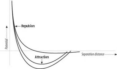
In physics, the Lenard-Jones potential represents the potential energy of attraction and repulsion between molecules. Here, U represents the interatomic potential energy, which is inversely proportional to the separation distance, r, between molecules. A and B are parameters, as are the exponents m and n. If we take the derivative of this potential function, we get a function representing a force. The force function produces both attractive and repulsive forces depending on the proximity of two molecules, or in our case game units, being acted upon. It’s this ability to represent both attractive and repulsive forces that will benefit us; however, instead of molecules, we’re going to deal with computer-controlled units.

So, what can we do with this ability to attract or repel computer-controlled units? Well, first off we can use the Lenard-Jones function to cause our computer-controlled unit to be attracted to the player unit so that the computer-controlled unit will chase the player. We also can tweak the parameters of the potential function to cause the computer-controlled unit to be repelled by the player, thus causing it to evade the player. Further, we can give any number of player units various weights to cause some of them to be more attractive or repulsive to the computer-controlled units than others. This will give us a means of prioritizing targets and threats.

In addition to chasing and evading, we can apply the same potential function to cause the computer-controlled units to avoid obstacles. Basically, the obstacles will repel the computer-controlled units when in close proximity, causing them to essentially steer away from them. We even can have many computer-controlled units attract one another to form a swarm. We then can apply other influences to induce the swarm to move either toward or away from a player or some other object and to avoid obstacles along the way.

The cool thing about using the Lenard-Jones potential function for these tasks is that this one simple function enables us to create all sorts of seemingly intelligent behavior.

To show how to implement potential-based chasing (or evading), we need only add a few bits of code to AIDemo2-2 (see Chapter 2 for more details). In that example program, we simulated the predator and prey units in a continuous environment. The function UpdateSimulation was responsible for handling user interaction and for updating the units every step through the game loop. We’re going to add two lines to that function, as shown in Example 5-1.

Lenard-Jones Potential Function

The following equation shows the Lenard-Jones potential function:

In solid mechanics, U represents the interatomic potential energy, which is inversely proportional to the separation distance, r, between molecules. A and B are parameters, as are the exponents m and n. To get the interatomic force between two molecules, we take the negative of the derivative of this potential function, which yields:

Here, again, A, B, m, and n are parameters that are chosen to realistically model the forces of attraction and repulsion of the material under consideration. For example, these parameters would differ if a scientist were trying to model a solid (e.g., steel) versus a fluid (e.g., water). Note that the potential function has two terms: one involves −A/r ⁿ, while the other involves B/r ^m. The term involving A and n represents the attraction force component of the total force, while the term involving B and m represents the repulsive force component.

The repulsive component acts over a relatively short distance, r, from the object, but it has a relatively large magnitude when r gets small. The negative part of the curve that moves further away from the vertical axis represents the force of attraction. Here, the magnitude of the force is smaller but it acts over a much greater range of separation, r.

You can change the slope of the potential or force curve by adjusting the n and m parameters. This enables you to adjust the range over which repulsion or attraction dominates and affords some control over the point of transition. You can think of A and B as the strength of the attraction and repulsion forces, respectively, whereas the n and m represent the attenuation of these two force components.

void	     UpdateSimulation(void)
{
     double	dt = _TIMESTEP;
     RECT	r;
     // User controls Craft1:
     Craft1.SetThrusters(false, false);
	
     if (IsKeyDown(VK_UP))
              Craft1.ModulateThrust(true);
	
     if (IsKeyDown(VK_DOWN))
              Craft1.ModulateThrust(false);
		
     if (IsKeyDown(VK_RIGHT))
     	        Craft1.SetThrusters(true, false);
     if (IsKeyDown(VK_LEFT))
    	         Craft1.SetThrusters(false, true);
     // Do Craft2 AI:
     .
     .
     .
     if(PotentialChase)
               DoAttractCraft2();
     // Update each craft's position:
     Craft1.UpdateBodyEuler(dt);
     Craft2.UpdateBodyEuler(dt);
     // Update the screen:	
     .
     .
     .
}

As you can see, we added a check to see if the PotentialChase flag is set to true. If it is, we execute the AI for Craft2, the computer-controlled unit, which now uses the potential function. DoAttractCraft2 handles this for us. Basically, all it does is use the potential function to calculate the force of attraction (or repulsion) between the two units, applying the result as a steering force to the computer-controlled unit. Example 5-2 shows DoAttractCraft2.

// Apply Lenard-Jones potential force to Craft2
void     DoAttractCraft2(void)
{
     Vector  r = Craft2.vPosition - Craft1.vPosition;
     Vector  u = r;
     u.Normalize();
     double  U, A, B, n, m, d;
     A = 2000;
     B = 4000;
     n = 2;
     m = 3;
     d = r.Magnitude()/Craft2.fLength;
     U = -A/pow(d, n) + B/pow(d, m);
     Craft2.Fa = VRotate2D( -Craft2.fOrientation, U * u);
     Craft2.Pa.x = 0;
     Craft2.Pa.y = Craft2.fLength / 2;
     Target = Craft1.vPosition;
}

The code within this function is a fairly straightforward implementation of the Lenard-Jones function. Upon entry, the function first calculates the displacement vector between Craft1 and Craft2. It does this by simply taking the vector difference between their respective positions. The result is stored in the vector r and a copy is placed in the vector u for use later. Note that u also is normalized.

Next, several local variables are declared corresponding to each parameter in the Lenard-Jones function. The variable names shown here directly correspond to the parameters we discussed earlier. The only new parameter is d. d represents the separation distance, r, divided by the unit’s length. This yields a separation distance in terms of unit lengths rather than position units. This is done for scaling purposes, as we discussed in Chapter 4.

Aside from dividing r by d, all the other parameters are hardcoded with some constant values. You don’t have to do it like this, of course; you could read those values in from some file or other source. We did it this way for clarity. As far as the actual numbers go, they were determined by tuning—i.e., they all were adjusted by trial and error until the desired results were achieved.

The line that reads U = −A/pow(d, n) + B/pow(d, m); actually calculates the steering force that will be applied to the computer-controlled unit. We used the symbol U here, but keep in mind that what we really are calculating is a force. Also, notice that U is a scalar quantity that will be either negative or positive, depending on whether the force is an attractive or repulsive force. To get the force vector, we multiply it by u, which is a unit vector along the line of action connecting the two units. The result is then rotated to a local coordinate system connected to Craft2 so that it can be used as a steering force. This steering force is applied to the front end of Craft2 to steer it toward or away from the target, Craft1. That’s all there is to it.

Upon running this modified version of the chase program, we can see that the computer-controlled unit does indeed chase or evade the player unit depending on the parameters we’ve defined. Figure 5-2 shows some of the results we generated while tuning the parameters.

Figure 5-2. Potential chase and evade

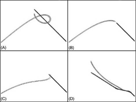
In Figure 5-2 (A), the predator heads toward the prey and then loops around as the prey passes him by. When the predator gets too close, it turns abruptly to maintain some separation between the two units. In Figure 5-2 (B), we reduced the strength of the attraction component (we reduced parameter A somewhat), which yielded behavior resembling the interception algorithm we discussed in Chapter 2. In Figure 5-2 (C), we increased the strength of attraction and the result resembles the basic line-of-sight algorithm. Finally, in Figure 5-2 (D), we reduced the attraction force, increased the repulsion force, and adjusted the exponent parameters. This resulted in the computer-controlled unit running from the player.

Adjusting the parameters gives you a great deal of flexibility when tuning the behavior of your computer-controlled units. Further, you need not use the same parameters for each unit. You can give different parameter settings to different units to lend some variety to their behavior—to give each unit its own personality, so to speak.

You can take this a step further by combining this potential function approach with one of the other chase algorithms we discussed in Chapter 2. If you play around with AIDemo2-2, you’ll notice that the menu selections for Potential Chase and the other chase algorithms are not mutually exclusive. This means you could turn on Potential Chase and Basic Chase at the same time. The results are very interesting. The predator relentlessly chases the prey as expected, but when it gets within a certain radius of the prey, it holds that separation—i.e., it keeps its distance. The predator sort of hovers around the prey, constantly pointing toward the prey. If the prey were to turn and head toward the predator, the predator would turn and run until the prey stops, in which case the predator would resume shadowing the prey. In a game, you could use this behavior to control alien spacecraft as they pursue and shadow the player’s jet or spacecraft. You also could use such an algorithm to create a wolf or lion that stalks its victim, keeping a safe distance until just the right moment. You even could use such behavior to have a defensive player cover a receiver in a football game. Your imagination is the only limit here, and this example serves to illustrate the power of combining different algorithms to add variety and, hopefully, to yield some sort of emergent behavior.

As you’ve probably already realized, we can use the repelling nature of the Lenard-Jones function to our advantage when it comes to dealing with obstacles. In this case, we set the A parameter, the attraction strength, to 0 to leave only the repulsion component. We then can play with the B parameter to adjust the strength of the repulsive force and the m exponent to adjust the attenuation—i.e., the radius of influence of the repulsive force. This effectively enables us to simulate spherical, rigid objects. As the computer-controlled unit approaches one of these objects, a repulsive force develops that forces the unit to steer away from or around the object. Keep in mind that the magnitude of the repulsive force is a function of the separation distance. As the unit approaches the object, the force might be small, causing a rather gradual turn. However, if the unit is very close, the repulsive force will be large, which will force the unit to turn very hard.

In AIDemo5-1, we created several randomly placed circular objects in the scene. Then we created a computer-controlled unit and set it in motion along an initially random trajectory. The idea was to see if the unit could avoid all the obstacles. Indeed, the unit did well in avoiding the objects, as illustrated in Figure 5-3.

Figure 5-3. Obstacle avoidance

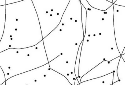
Here, the dark circles represent obstacles, while the swerving lines represent the trails the computer-controlled unit left behind as it navigated the scene. It’s clear from this screenshot that the unit makes some gentle turns to avoid objects that are some distance away. Further, it takes some rather abrupt turns when it finds itself in very close proximity to an object. This behavior is very similar to what we achieved in the flocking examples in the previous chapter; however, we achieved the result here by using a very different mechanism.

How all this works is conceptually very simple. Each time through the game loop all the objects, stored in an array, are cycled through, and for each object the repulsion force between it and the unit is calculated. For many objects the force is small, as they might be very far from the unit, whereas for others that are close to the unit the force is much larger. All the force contributions are summed, and the net result is applied as a steering force to the unit. These calculations are illustrated in Example 5-3.

void     DoUnitAI(int i)
{
          int              j;
          Vector          Fs;
          Vector          Pfs;
          Vector          r, u;
          double          U, A, B, n, m, d;
          Fs.x = Fs.y = Fs.z = 0;
          Pfs.x = 0;
          Pfs.y = Units[i].fLength / 2.0f;
          .
          .
          .
          if(Avoid)
          {
               for(j=0; j<_NUM_OBSTACLES; j++)
               {
                    r = Units[i].vPosition - Obstacles[j];
                    u = r;
                    u.Normalize();
                    A = 0;
                    B = 13000;
                    n = 1;
                    m = 2.5;
                    d = r.Magnitude()/Units[i].fLength;
                    U = -A/pow(d, n) + B/pow(d, m);
                    Fs += VRotate2D( -Units[i].fOrientation,
                                          U * u);
               }
          }
          Units[i].Fa = Fs;
          Units[i].Pa = Pfs;
}

The force calculation shown here is essentially the same as the one we used in the chase example; however, in this case the A parameter is set to 0. Also, the force calculation is performed once for each object, thus the force calculation is wrapped in a for loop that traverses the Obstacles array.

You need not restrict yourself to circular or spherical obstacles. Although the repulsion force does indeed have a spherical influence, you can effectively use several of these spheres to approximate arbitrarily shaped obstacles. You can line up several of them and place them close to one another to create wall boundaries, and you even can group them using different attenuation and strength settings to approximate virtually any shape. Figure 5-4 shows an example of how to use many small, spherical obstacles to represent a box within which the unit is free to move.

Figure 5-4. Boxed in

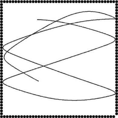
In this case, we simply took example AIDemo5-1 and distributed the obstacles in a regular fashion to create a box. We used the same algorithm shown in Example 5-3 to keep the unit from leaving the box. The trail shown in Figure 5-4 illustrates the path the unit takes as it moves around the box.

Granted, this is a simple example, but it does illustrate how you can approximate nonspherical boundaries. Theoretically, you could distribute several spherical obstacles around a racetrack to create a boundary within which you want a computer-controlled race car to navigate. These boundaries need not be used for the player, but would serve only to guide the computer-controlled unit. You could combine such boundaries with others that only attract, and then place these strategically to cause the computer-controlled unit to be biased toward a certain line or track around the racecourse. This latter technique sort of gets into waypoints, which we’ll address later.

Let’s consider group behavior as yet another illustration of how to use potential functions for game AI. Specifically, let’s consider swarming. This is similar to flocking, however the resulting behavior looks a bit more chaotic. Rather than a flock of graceful birds, we’re talking about something more like an angry swarm of bees. Using potential functions, it’s easy to simulate this kind of behavior. No rules are required, as was the case for flocking. All we have to do is calculate the Lenard-Jones force between each unit in the swarm. The attractive components of those forces will make the units come together (cohesion), while the repulsive components will keep them from running over each other (avoidance).

Example 5-4 illustrates how to create a swarm using potential functions.

void     DoUnitAI(int i)
{
          int             j;
          Vector   Fs;
          Vector   Pfs;
          Vector   r, u;
          double   U, A, B, n, m, d;
          // begin Flock AI
          Fs.x = Fs.y = Fs.z = 0;
          Pfs.x = 0;
          Pfs.y = Units[i].fLength / 2.0f;
          if(Swarm)
          {
               for(j=1; j<_MAX_NUM_UNITS; j++)
               {
                    if(i!=j)
                    {
                         r = Units[i].vPosition -
                             Units[j].vPosition;
                         u = r;
                         u.Normalize();
                         A = 2000;
                         B = 10000;
                         n = 1;
                         m = 2;
                         d = r.Magnitude()/
                                    Units[i].fLength;
                         U = -A/pow(d, n) +
                                    B/pow(d, m);
                         Fs += VRotate2D(
                                         -Units[i].fOrientation,
                                         U * u);
                    }
               }
          }
          Units[i].Fa = Fs;
          Units[i].Pa = Pfs;
          // end Flock AI
}

Here, again, the part of this code that calculates the force acting between each unit with every other unit is the same force calculation we used in the earlier examples. The main difference here is that we have to calculate this force between each and every unit. This means we’ll have nested loops that index the Units array calculating the forces between Units[i] and Units[j], so long as i is not equal to j. Clearly this can result in a great many computations as the number of units in the swarm gets large. Later we’ll discuss a few things that you can do to optimize this code.

For now, take a look at Figure 5-5, which illustrates the resulting swarming behavior.

Figure 5-5. Swarm

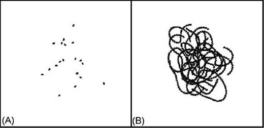
It’s difficult to do justice to the swarm with just a snapshot, so you should download the example program and try it for yourself to really see what the swarm looks like. In any case, Figure 5-5 (A) illustrates how the units have come together. Figure 5-5 (B) shows the paths each unit took. Clearly, the paths swirl and are intertwined. Such behavior creates a rather convincing-looking swarm of bees or flies.

You also can combine the chase and obstacle avoidance algorithms we discussed earlier with the swarming algorithm shown in Example 5-4. This would allow your swarms to not only swarm, but also to chase prey and avoid running into things along the way. Example 5-5 highlights what changes you need to make to the function shown in Example 5-4 to achieve swarms that chase prey and avoid obstacles.

void     DoUnitAI(int i)
{
          int              j;
          Vector    Fs;
          Vector    Pfs;
          Vector    r, u;
          double    U, A, B, n, m, d;
          // begin Flock AI
          Fs.x = Fs.y = Fs.z = 0;
          Pfs.x = 0;
          Pfs.y = Units[i].fLength / 2.0f;
          if(Swarm)
          {
               for(j=1; j<_MAX_NUM_UNITS; j++)
               {
                    if(i!=j)
                    {
                         r = Units[i].vPosition -
                             Units[j].vPosition;
                         u = r;
                         u.Normalize();
                         A = 2000;
                         B = 10000;
                         n = 1;
                         m = 2;
                         d = r.Magnitude()/
                              Units[i].fLength;
                         U = -A/pow(d, n) +
                               B/pow(d, m);
                         Fs += VRotate2D(
                                           -Units[i].fOrientation,
                                           U * u);
                    }
               }
          }
          if(Chase)
          {
               r = Units[i].vPosition - Units[0].vPosition;
               u = r;
               u.Normalize();
               A = 10000;
               B = 10000;
               n = 1;
               m = 2;
               d = r.Magnitude()/Units[i].fLength;
               U = -A/pow(d, n) + B/pow(d, m);
               Fs += VRotate2D( -Units[i].fOrientation, U * u);
          }
          if(Avoid)
          {
               for(j=0; j<_NUM_OBSTACLES; j++)
               {
                    r = Units[i].vPosition - Obstacles[j];
                    u = r;
                    u.Normalize();
                    A = 0;
                    B = 13000;
                    n = 1;
                    m = 2.5;
                    d = r.Magnitude()/Units[i].fLength;
                    U = -A/pow(d, n) + B/pow(d, m);
                    Fs += VRotate2D( -Units[i].fOrientation,
                                          U * u);
               }
          }
          Units[i].Fa = Fs;
          Units[i].Pa = Pfs;
          // end Flock AI
}

Here, again, the actual force calculation is the same as before, and in fact we simply cut and pasted the highlighted blocks of code from the earlier examples into this one.

Swarms are not the only things for which you can use this algorithm. You also can use it to model crowd behavior. In this case, you’ll have to tune the parameters to make the units move around a little more smoothly rather than erratically, like bees or flies.

Finally, we should mention that you can combine leaders with this algorithm just as we did in the flocking algorithms in the previous chapter. In this case, you need only designate a particular unit as a leader and have it attract the other units. Interestingly, in this scenario as the leader moves around, the swarm tends to organize itself into something that resembles the more graceful flocks we saw in the previous chapter.

You’ve probably already noticed that the algorithms we discussed here can become quite computationally intensive as the number of obstacles or units in a swarm increases. In the case of swarming units, the simple algorithm shown in Examples 5-4 and 5-5 is of order N² and would clearly become prohibitive for larger numbers of units. Therefore, optimization is very important when actually implementing these algorithms in real games. To that end, we’ll offer several suggestions for optimizing the algorithms we discussed in this chapter. Keep in mind that these suggestions are general in nature and their actual implementation will vary depending on your game architecture.

The first optimization you could make to the obstacle avoidance algorithm is to simply not perform the force calculation for objects that are too far away from the unit to have any influence on it. What you could do here is put in a quick check on the separation distance between the given obstacle and the unit, and if that distance is greater than some prescribed distance, skip the force calculation. This potentially could save many division and exponent operations.

Another approach you could take is to divide your game domain into a grid containing cells of some prescribed size. You could then assign each cell an array to store indices to each obstacle that falls within that cell. Then, while the unit moves around, you can readily determine which cell it is in and perform calculations only between the unit and those obstacles contained within that cell and the immediately adjacent cells. Now, the actual size and layout of the cells would depend on your specific game, but generally such an approach could produce dramatic savings if your game domain is large and contains a large number of obstacles. The tradeoff here is, of course, increased memory requirements to store all the lists, as well as some additional bookkeeping baggage.

You could use this same grid-and-cell approach to optimize the swarming algorithm. Once you’ve set up a grid, each cell would be associated with a linked list. Then, each time through the game loop, you traverse the unit’s array once and determine within which cell each unit lies. You add a reference to each unit in a cell to that particular cell’s linked list. Then, instead of going through nested loops, comparing each unit with every other unit, you need only traverse the units in each cell’s list, plus the lists for the immediately adjacent cells. Here, again, bookkeeping becomes more complicated, but the savings in CPU usage could be dramatic. This optimization technique is commonly applied in computational fluid dynamics algorithms and effectively reduces order N² algorithms to something close to order N.

One final suggestion we can offer is based on the observation that the force between each pair of units is equal in magnitude but opposite in direction. Therefore, once you’ve calculated the force between the pair of units i and j, you need not recalculate it for the pair j and i. Instead, you apply the force to i and the negative of the force to j. You’ll of course have to do some bookkeeping to track which unit pairs you’ve already addressed so that you don’t double up on the forces.